Vol. 1, No. 1, November 2003, 61 - 69
Interface Identification in
Magnetic Fluid Dynamics
Marek Ziolkowski
1, Hartmut Brauer
2, Milko Kuilekov
3Abstract: In magnetic fluid dynamics appears the problem of reconstruction of free boundary between conducting fluids, e.g. in aluminum electrolysis cells. We have investi-gated how the interface between two fluids of different conductivity of a highly simplified model of an aluminum electrolysis cell could be reconstructed by means of external mag-netic field measurements using simple gemag-netic algorithm.
Keywords: Genetic algorithms, Optimisation simulations, Inverse solution, Interface re-construction.
1 Introduction
There are a variety of problems in material processing where it would be useful to know the time-dependent distribution of the electrical conductivity of a single fluid or a multiphase flow. For instance, the knowledge of the position of the interface between highly conducting molten aluminum and poorly conducting liquid cryolite is important to prevent unwelcome instabilities in aluminum reduction cells [1]. Other examples in-clude electrical conductivity distributions in glass melting furnaces, metal-slag interfaces in steel and iron making as well as online detection of inclusions. The liquids involved in material processing such as molten metals, semiconductors, and glass melts are mostly hot and highly aggressive. Therefore, conventional measurement techniques em-ploying local probes face serious difficulties.
The purpose of the present work is to demonstrate that concepts of Magnetic Field
Tomography (MFT) which have been successfully applied to a variety of problems in
biomagnetism [2] can be used in order to detect interfaces between current carrying flu-ids of different electrical conductivity [3, 4]. We demonstrate that the external magnetic field generated by the electrical current flowing through a highly simplified model of an aluminum reduction cell provides sufficient information to reconstruct the unknown interface shape.
1
Technische Universitaet Ilmenau, Helmholtzplatz 2, D-98684 Ilmenau, Deutschland, and Technical University of Szczecin, Sikorskiego 37, PL-70313, Poland,
E-mail: [email protected]
2
Technische Universitaet Ilmenau, Helmholtzplatz 2, D-98684 Ilmenau, Deutschland, E-mail: [email protected]
3
62
2 Highly Simplified Cell Model
Electrolysis produces chemical changes in a material by generating an otherwise unachievable chemical reaction by means of electrical energy. In the production of pri-mary aluminum, alumina (Al2O3) is dissolved in an electrolyte that consists of molten
fluoride salts kept at about 960 °C. When direct current is passed through this mixture, the alumina is decomposed into molten aluminum, deposited at the cathode, and oxygen, which reacts with the carbon anode to form CO2.
Although the principles of this process have remained unchanged for more than 100 years, the performance of the electrolytic cells has been vastly improved. Today the best cells operate with energy efficiencies about 50 %, which is above average for electro-lytic processes in molten salts. One of the keys to further improvements in energy effi-ciency and productivity is a better understanding of the chemical and physical conditions prevailing in the cells [5-7].
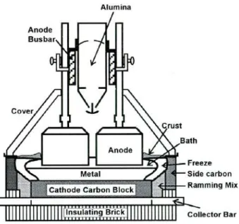
Fig. 1 - Scheme of an aluminum reduction cell.
If we consider typical figures of aluminum electrolysis cells (Fig.1) it must be no-ticed that the cross section has a length of about L= 8 m, whereas the interface displace-ment η is very small compared to the lateral extent of the system. Industrial practice shows that already such small interface displacement can perturb significantly the op-eration of the cell [8]. Consequently, our physical model is characterized by a very small ratio η/L.
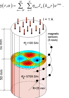
The considered highly simplified problem is shown in Fig.2. Two fluids with dif-ferent electrical conductivity σ2 (up) and σ1 (down) are situated in a long cylinder of the
The complete interface perturbation can be found solving the Euler equation and the mass conservation law,
(
)
(
)
1
,
M N
jm mn m mn m M n
r
J
k r e
αη
α
η
=− =
=
∑ ∑
. (1)Fig. 2 - Highly simplified aluminum reduction cell model – cylinder with two conducting fluids.
The value n is called the radial mode number and the value m the azimuthal mode number. Using this notation we call ηmn as an mn-mode e.g. η12 denotes mode 12
(Fig.3).
64
Although the quantity of modes is usually unlimited, the highest modes have small amplitudes and therefore can be neglected.
The validity of the above interface representation is limited by the amplitude of the interface oscillations. We consider only small interface oscillations because the larger interface oscillations lead to instabilities due to drop formation [8].
3 Magnetic Field Modelling
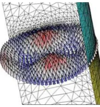
If the interface between fluids is flat, the current density J is homogeneous every-where. As soon as the interface deviates from its flat shape, due to interfacial waves or an external forcing, the current density J will become inhomogeneous near the interface (Fig.4).
The inhomogeneity of J is represented by the perturbation current density j. If the perturbation of the fluid interface is non-axisymmetric, it leads to a perturbation of the radial and axial component of the magnetic field outside the cylinder. This fact is used for the interface reconstructions.
Fig. 4 - Current density distribution near the interface.
To model the magnetic field, first, we have formulated the problem using the scalar electric potential Φ,
0
φ
, 0 J z0 /σ
Φ = Φ + Φ = ,
which fulfils the Laplace equations,
,
with the following boundary and interface conditions,
1 2
0,r R 0, z H/ 2
r
φ
φ
φ
∂
= = = = = ±
∂
and
1⋅ = 2⋅ , Φ = Φ1 2
In the case of analytical approach (applicable only to small perturbations) the fol-lowing linearized interface condition has been formulated [9, 10],
.
.
.
.
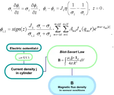
Fig. 5 - Flowchart of forward calculations using analytical method.
Fig. 6 - Flowchart of forward calculations using finite element method. Having electric potential φ we can calculate the perturbation current density distri-bution j in the cylinder and then, applying the Biot-Savart law, the magnetic flux density in the sensors area (Fig.5). To avoid the limits with the perturbation amplitude the nu-merical method has to be applied. We have chosen the finite element method in which first order tetrahedral elements have been used. Fig.6 shows the flowchart of calcula-tions of the magnetic flux density distribucalcula-tions in the sensor area in the case when the finite element method is used.
Geometry model
BC
setting
Meshing Domains description
Iterative solver
Good Broyden with ICCG preconditioner Extract current density Biot-Savart Law B
Magnetic flux density in sensor positions Problem definition:
3D Conductive media DC
FEMLAB® FEM3D 0 2 4 R V dV R µ ×
=∫ J 1
B E
Elleeccttrriiccppootteennttiiaalφlφ
-σ∇(⋅)
C
Cuurrrreennttddeennssiittyyjj
i
innccyylliinnddeer r
Biot-Savart Law
B
Magnetic flux density in sensor positions
0 2 4 R V dV R µ π ×
=
∫
j 166
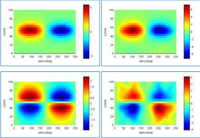
Fig.7 shows the distribution of magnetic flux density components (Br, Bz) on the
evolved cylindrical surface of the radius 35 mm calculated with analytical and numerical methods.
Fig. 7 - Distribution of magnetic flux density, Br (up) and Bz (down) components
calculated by analytical (left) and FEM (right) methods.
The differences observed in Fig.7 (shift of extreme positions) between analytical and numerical distributions of magnetic flux density come from the fact that applied linearized interface condition in the analytical method cause the elimination of the an-gular non-symmetry of the current density distribution in the vicinity of the interface. It means that for higher radial modes (n>2) only the numerical methods could give correct results in modelling of magnetic field distributions in the sensor area.
4 Interface Reconstruction
The reconstructions of the interface shape have been performed on the simulated data.
Fig. 8 - Flowchart of the interface shape reconstruction.
Add Noise Y/N
Sensors reductor
ns(nr)=8(1), 8(3), 8(5) …
Magnetic field map Forward solver
Analytical/FEM
Mode
FFT Y/N
Simulated data
CF <ε
GA
-no of generations -population size -mutation probability
Best field
According to Fig.8, first, we have to define the mode, which describes the interface shape, then, the magnetic flux density in the sensors positions (72 sensors in 21 rows) is calculated (as it is shown in the previous section). In the next step, the white noise has been added to the magnetic field. Sample distribution of the noisy Br component of the
magnetic flux density is shown in Fig.9.
Fig. 9 - Distribution of Br component with 20% white noise.
Due to limited number of sensors, which could be used in the experiment (maxi-mum 8 sensors in one row, Fig.10), the calculated data has to be reduced and located to the prescribed sensor positions.
35mm 25mm Cylinder
Fig. 10-Ring with 8 2D sensors (Br & Bz components).
After reduction process, the sample distribution of the magnetic flux density for 8 sensors in one row and 5 rows with 20 mm distance between rows is shown in Fig.11.
The reconstruction process is realized in two steps. First, the fast Fourier transfor-mation (FFT) of the simulated data is calculated and the significant azimuthal modes are identified. Next, the radial modes have been found using simple genetic algorithm (GA) [11].
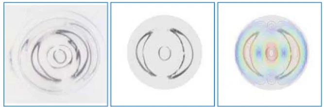
As an example, we have reconstructed the shape of the interface described by mode
η12. That mode has been chosen due to the analysis of the first experiment results shown in Fig.12.
posi-68
tions. The result of reconstruction is shown in Fig.13. In that case, the population size was equal 30, the mutation probability 0.01, and the crossover probability 0.6.
Fig. 11- Br & Bz distribution with 20% noise for 8 sensors in 5 rows.
Fig. 12 - Photo snapshot of the interface surface (experiment) compared with the curvature distribution of η12 mode.
Fig. 13 - Original η12 mode (left) and the interface shape (right)
reconstructed from the noisy Br & Bz distribution.
5 Conclusion
real experimental data. In that case, the simple FFT block has to be completed with the DSP block which could improve the signal to noise ratio.
References
[1] P. A. Davidson: Magnetohydrodynamics in material processing, Annu. Rev. Fluid Mech., vol. 31, pp. 273 - 300, 1999.
[2] H. Brauer, J. Haueisen, M. Ziolkowski, U. Tenner, H. Nowak: Reconstruction of extended current sources in a human body phantom applying biomagnetic measur-ing techniques, IEEE Transaction on Magnetics, vol. 36, No. 4, pp. 1700 -1705, 2000.
[3] P. A. Davidson: Magnetohydrodynamics in material processing, Annu. Rev. Fluid Mech., vol. 31, pp. 273 - 300, 1999.
[4] K. Fujisaki, K. Wajima, T. Ohki: 3-D magnetohydrodynamics analysis method for free surface molten metal, IEEE Transaction on Magnetics, vol. 36, No. 4, pp. 1325 - 1328, 2000.
[5] A. Bojarevics, V. Bojarevics, Y. Gelfgat, K. Pericleous: Liquid metal turbulent flow dynamics in a cylindrical container with free surface: experiment and numerical analysis, Magnitnaya Gidrodinamika, vol. 35, No. 3, pp. 258 - 277, 1999.
[6] I. Panaitescu, M. Repetto, L. Leboucher, K. Pericleous: Magneto-hydro-dynamic analysis of an electrolysis cell for aluminum production, IEEE Transaction on Mag-netics, vol. 36, No. 4, pp. 1305 - 1308, 2000.
[7] V. Chechurin, A. Kalimov, L. Minevich, M. Svedentsov, M. Repetto: A simulation of magneto-hydrostatic phenomena in thin liquid layers of an aluminum electrolytic cell, IEEE Transaction on Magnetics, vol. 36, No. 4, pp. 1309 - 1312, 2000.
[8] J. Miles, D. Henderson: Parametrically forced surface waves, Annu. Rev. Fluid Mech., vol. 22, pp. 143 - 165, 1990.
[9] A. Kurenkov, A. Thess: Reconstruction of interfaces between electrically conduct-ing fluids from electrical potential measurements, 4th Int. Conf. of Magnetohydro-dynamics, Giens/France, September 2000, Proc. vol. 1, pp. 45 - 50, 2000.
[10] H. Brauer, M. Ziolkowski, M. Dannemann, M. Kuilekov, D. Alexeevski: Forward Simulations for Free Boundary Reconstruction in Magnetic Fluid Dynamics, COM-PEL, vol. 22, no 3, 2003 (to be published).