SRef-ID: 1607-7946/npg/2004-11-567
Nonlinear Processes
in Geophysics
© European Geosciences Union 2004
Developments in the theory of collisionless reconnection in magnetic
configurations with a strong guide field
F. Pegoraro1, D. Borgogno2, F. Califano1, D. Del Sarto1, E. Echkina3, D. Grasso2, T. Liseikina4, and F. Porcelli2
1Phys. Dept., University of Pisa and INFM, Pisa Italy
2BPRG-INFM, Dept. of Energetics, Politecnico di Torino, Torino, Italy 3Moscow State University, Moscow, Russia
4Institute of Computational Technologies SD RAS, Novosibirsk, Russia
Received: 7 September 2004 – Revised: 9 November 2004 – Accepted: 12 November 2004 – Published: 19 November 2004 Part of Special Issue “Advances in space environment turbulence”
Abstract.We review some recent results that have been ob-tained in the investigation of collisionless reconnection in two dimensional magnetic configurations with a strong guide field in regimes of interest for laboratory plasmas. First we adopt a two-fluid dissipationless plasma model where the plasma evolution is described by the advection of two Lagrangian invariant fields. Then, we show that an analo-gous formulation in terms of Lagrangian invariants applies to the case where the electron response is obtained from a drift-kinetic model.
1 Introduction
Laboratory plasmas and space plasmas often exhibit different physical behaviour even in the case of closely related phe-nomena, such as magnetic field line reconnection, because of different parameter ratios and most importantly, because of different boundary conditions. In particular, laboratory plasmas are strongly constrained by periodicity conditions and, with the exception of Reverse Field Pinches, by the structural rigidity imposed by the externally generated and quasi-uniform toroidal magnetic field. On the other hand both types of plasmas are generally characterized by very large Lundquist numbers and, in particular for space plasmas, by conditions where the characteristic reconnection time is shorter than the electron-ion collision time. In such low col-lisionality regimes magnetic reconnection is made possible not by electron resistivity, but by electron inertia and by ki-netic (thermal) effects.
Recently, collisionless magnetic field line reconnection in the laboratory has been re-examined in Ottaviani et al. (1993, 1995); Cafaro et al. (1998); Grasso et al. (2000, 2001); Por-celli et al. (2002); Del Sarto et al. (2003); Pegoraro et al.
Correspondence to:F. Pegoraro ([email protected])
(2004) and in Liseikina et al. (2004) with the aim of un-derstanding the fast evolution time scales displayed in the experiments and of determining whether the magnetic is-land growth can saturate in the absence of dissipation. Of particular importance is the investigation of whether and in which form the reconnection time scales are determined by the microscopic spatial scales arising from electron inertial and thermal effects and that are involved in the reconnec-tion process (see, e.g. Bhattacharjee et al., 2001; Shay et al., 2001; Wang et al., 2001; Fitzpatrick, 2004a,b). In addition, it is important to investigate whether the relative values of these microscopic spatial scales determine:
1) the final state of the saturated island and in particular the distribution of the current layers and of the fluid vortic-ity layers within the island,
2) the redistribution of the released magnetic energy among the different forms of plasma energy,
3) the onset of secondary instabilities driven by the recon-nection process.
to the kinetic regime is imposed by the fact that, in the pres-ence of thermal effects, a fluid approach cannot be properly justified at the increasingly small scale lengths that are char-acteristic of the plasma nonlinear evolution in the absence of dissipation.
An important consequence of the results reviewed in this paper is that the physical process that occur at the micro-scopic scalelengths involved in the reconnection process de-termine its evolution in a very intrinsic way by changing the conservation laws that the plasma evolution must obey. This is very different from the case when magnetic reconnection occurs through the effect of electron resistivity, as in the lat-ter case no invariant quantities are preserved.
2 Magnetic connections
Magnetic topology plays an important role in the global dy-namics of high temperature plasmas. Within the ideal MHD plasma description, where
E+u×B/c=0, ⇒ ∂B
∂t = ∇ ×(u×B) , (1)
withE(x, t ),B(x, t )the plasma electric and magnetic field andu(x, t )the fluid plasma velocity, two plasma elements, separated by the vectorδl(x, t )that are initially connected by a magnetic field line (δl×B=0 att=0), remain connected by a field line at any subsequent time, sinceδl×Bis transported with the plasma (i.e., its Lie derivative vanishes)
∂(δl×B)
∂t +(u· ∇) (δl×B)= −(∇u)·(δl×B) . (2)
This condition introduces a topological linking (magnetic connection) between plasma elements that is preserved dur-ing the ideal MHD plasma evolution. Magnetic linkdur-ing con-straints the plasma dynamics by making configurations with lower magnetic energy, but different topological linking, in-accessible.
Magnetic reconnection partially removes these constrains by allowing the field lines to decouple locally (i.e., around critical points) from the plasma motion and to reknit in a dif-ferent net of connections. This localized breaking of the con-nections arises from physical effects neglected in Eq. (1) that are weak all over the plasma, but are locally enhanced by the formation of small spatial scales around critical points.
In collisionless magnetic field line reconnection, the de-coupling between the magnetic field and the plasma motion occurs because of finite electron inertia (in the fluid limit) or thermal effects (in the kinetic plasma description). In the absence of dissipation, the plasma response both in the fluid and in the kinetic electron treatment admits generalized link-ing conditions that are preserved durlink-ing the process of mag-netic reconnection and that in a 2-D configuration take the simple form of Lagrangian invariants.
2.1 Generalized magnetic connections: an example In a collisionless cold plasma model the effect of electron inertia and of the Hall term in Ohm’s law
E+u
c ×B= − me
e due
dt +
1
necJ×B, (3)
can be accounted for by introducing the vector fields Be≡B−mec
e ∇ ×ue= ∇ ×Ae, (4)
Ee≡E+me 2e∇u
2
e+
me
e ∂ue
∂t = −∇ϕe−
1
c ∂Ae
∂t , (5)
where subscriptsedenote electron quantities and ue is the electron fluid velocity. The generalized vector potentialAe is proportional to the fluid electron canonical momentum and
ϕeto the total electron energy and reduce to vector potential
Aand to the electrostatic potentialϕin the limit of massless electrons. The vector fieldsBe(x, t )andEe(x, t )satisfy the homogeneous Mawxell’s equations and the ideal Ohm’s law in the form
Ee+ue
c ×Be=0, (6)
which leads to the generalized liking condition
∂(δl×Be)
∂t +(ue·∇) (δl×Be)= −(∇ue)·(δl×Be) . (7)
Similarly, all the ideal MHD theorems (magnetic flux conser-vation, magnetic helicity conserconser-vation, linking number etc,) are recovered by substitutingBeforBandueforu.
2.2 Transitions between magnetic equilibria
The breaking of the magnetic connections allows the system to access configurations with lower magnetic energy.
3 Two-dimensional configurations: connections and Lagrangian invariants
The concept of magnetic connections simplifies in the case of two-dimensional (2-D) configurations where all quantities depend onx,yand on timet only. The magnetic configura-tions of interest here are characterized by a strong, externally imposed, Bz field which is taken to be fixed and does not
play the role of a dynamical variable and by an inhomoge-neous shear field in the x−y plane associated with a current densityJ (x, y, t )along the z-axis. The fieldBzplays a very
important physical role in determining the model that is ap-propriate to represent the plasma dynamics in the x−y plane. Plasma configurations whereBzis absent display a different
behaviour both in the fluid and in the kinetic description. In such a 2-D configuration, the magnetic and the electric field can be expressed as
B=B0ez+ ∇ψ (x, y, t )×ez, (8) E= −∇ϕ(x, y, t )+ez
c
∂ψ (x, y, t )
∂t , (9)
where the flux functionψ (x, y, t )is the z-component of the vector potential of the shear magnetic field andϕis the elec-trostatic potential which plays the role of the stream func-tion for the plama mofunc-tion in the x−y plane. Then, the con-served connections between plasma elements moving in the x−y plane take the form of Lagrangian invariants i.e., can be expressed in term of scalar quantities that are advected by the plasma motion and are constant along characteristics.
In the ideal MHD limit this Lagrangian invariant corre-sponds to the z component Az of the magnetic vector
po-tential i.e. to the flux functionψ. Plasma elements that lie initially on aψ=const curve in the x−y plane and that move along the characteristics of the stream functionϕ remain at all times on the sameψ=const curve, i.e.,ψ-connections are preserved. Note that the conservation of a Lagrangian invari-ant is qualitatively different from that expressed e.g. by the continuity equation for the plasma energy density, insofar as the values of a Lagrangian invariant cannot be modified, but only redistributed.
3.1 Cold fluid finite-mass electrons
If the effect of electron inertia is included (in a cold electron fluid), the Lagrangian invariant corresponds to the z compo-nentAz−(mec/e)ue,z of the “ vector potential” of the field
Be, which is proportional to the z component of the elec-tron canonical fluid momentum. In most cases of interest for magnetic reconnection in a configuration with a strong
Bzfield, the density perturbations can be taken to be small.
Then, the term proportional to the z componentue,z of the
electron velocity can be rewritten in terms of the z compo-nent of the electron current densityJ (we disregard the ion motion along field lines). Within this approximation, denot-ing as customaryAz−(mec/e)ue,zbyF, we have
F (x, y, t )=ψ (x, y, t )−de2∇2ψ (x, y, t ) , (10)
with−∇2ψ (x, y, t )≡J (x, y, t )the z component of the cur-rent density and de≡c/ωpe the collisionless electron skin
depth. The Lagrangian invariantF is advected by the stream functionϕof the electron motion in the x−y plane which is proportional to the electrostatic potential according to
∂F
∂t + [ϕ, F] =0, (11)
with the Poisson brackets[f, g]defined by
[f, g] =ez· ∇f × ∇g . (12)
This equation arises from the parallel component of Ohm’s Eq. (3). The stream functionϕobeys the equation
∂U
∂t + [ϕ, U] = [J, ψ], (13)
whereU=∇2ϕ is proportional to the plasma fluid vorticity
and to the plasma density perturbation. This equation arises from the electron continuity equation and from the quasi-neutrality condition, after expressing the ion perturbed den-sity in terms of the divergence of the ion polarization drift. 3.2 Warm fluid finite-mass electrons
When the effects of electron temperature are included, elec-tron parallel compressibility leads to a modification of the conserved connections (Schep et al., 1994) and introduces a new microscopic scale-lengthρs≡(me/mi)1/2vt he/ i the
so called ion-sound gyro-radius. When this contribution is included, an anisotropic electron pressure tensor appears in Ohm’s law (as shown in Schep et al. (1994), this term is needed in order to compensate for a drift term in the elec-tron inertia contribution). Then Eq. (11) becomes
∂F
∂t + [ϕ, F] =̺ 2
s[U, ψ], (14)
and the structure of the conserved connections is modified. By combining Eqs. (13, 14), we find that in this warm fluid finite-mass electron regime, two generalized connections are conserved which are expressed by the Lagrangian invariants
G±(x, y, t )defined by
G±=ψ−de2∇2ψ±deρs∇2ϕ , (15)
that are advected by the generalized stream functions
ϕ±=ϕ±(ρs/de)ψ . (16)
The new advection equations are
∂G±
∂t + [ϕ±, G±] =0. (17)
two “particle” species with opposite charges in the Poisson-type equation forϕ and equal charges in the Yukawa-type equation forψ
deρs∇2ϕ=
(G±−G±)
2 ,
ψ−de2∇2ψ= (G±+G±)
2 . (18)
The stream functionsϕ±play the role of the single particle Hamiltonians.
3.3 Dynamics: energy functional
The dynamics of the plasma configuration is governed by the conserved energy functionalHf l(ψ, ϕ)1
Hf l(ψ, ϕ)≡ Z d2x
2
|∇ψ|2+|∇ϕ|2+de2J2+̺2sU2. (19) The first termR
d2x|∇ψ|2/2 represents the magnetic energy
in the shear field,R
d2x|∇ϕ|2/2 the plasma fluid kinetic
mo-tion,R
d2xde2J2/2 the energy of the ordered electron kinetic energy along field lines andR
d2x̺2sU2/2 the work done by the parallel electron compression. This last term disappears in the limit of a cold electron fluid (̺s→0) . Note that the
magnetic energy and the plasma fluid kinetic motion, con-tain first derivatives orψ andϕ while the ordered electron kinetic energy and the work done by the parallel electron compression contain second derivatives, i.e., one can expect that the former two dominate at large scales and the latter two at small spatial scales. Note in addition that, in the ab-sence of dissipative effects, there are no characteristic dissi-pative scalelengths in Eqs. (17) that can limit the nonlinear formation of small spatial scales. However we stress that, even when “resistive” or “’viscous” effects are effectively in-cluded, they remain at all scales uniformly smaller than those of the electron inertial terms. This is guaranteed by the fact that fluid viscosity and electron resistivity do not introduce higher order differential operators in Eqs. (17) and that the characteristic evolution time is short on the the electron-ion collision time.
4 Nonlinear reconnection regimes
We are interested here in the nonlinear evolution of colli-sionless reconnection instabilities which arise because of the initial inhomogeneous current distribution in the x−y plane.
1This energy functional is related to the possibility of
describ-ing Eqs. (17) in the form of Hamiltonian field equations with non-canonical variables and degenerate non-non-canonical Poisson brackets (Morrison (1984); Kuvshinov et al. (1994)). The kernel of these Poisson brackets is given by an infinite set of Casimirs defined as
R
d2xC±(G±)withC±arbitrary smooth functions.
By redefining the energy functional Hf l by adding the ap-propriate combination of Casimirs, we can rewrite Hf l in the formH(G±, ϕ±)=−Rd2x (G+ϕ++G−ϕ−)/2 (Kuvshinov et al., 1998).
This procedure is different from the one where forced netic reconnection is studied in configurations where mag-netic flux is driven from their boundaries (in our case recon-nection is “forced” by the initial conditions). As mentioned above, the decoupling between the plasma motion and the magnetic field occurs around critical points that correspond, in the 2-D configurations under examination, to the zeros of the shear field i.e., to the zeros of∇ψ (x, y, t ). As is cus-tomary for magnetic configurations of interest for labora-tory plasmas, we consider initial configurations where crit-ical points have degenerated into a critcrit-ical line, i.e., initial configurations that depend only on one coordinate (say x) and where the shear field vanishes along a line (the null line):
ψ0=ψ0(x)with∂ψ0(x)/∂x=0|x=0.
The early development (linear phase) of the reconnection instabilities in such configurations has been thoroughly ex-amined in the literature in terms of threshold conditions for the onset of the instabilities, growth rates and role of the boundary layer at the null line. In this layer a large cur-rent density cumulates and the topology of the shear field starts to be changed with the formation of magnetic islands bounded by magnetic separatrices. The interest here is to examine the nonlinear phase of a collisionless reconnection instability and the eventual saturation of the island growth. The threshold condition of the reconnection instabilities in null line configurations is controlled by the value of a pa-rameter, usually denoted by1′, which “measures” both the total current that the instability drives in the boundary layer and the magnetic energy flux that is convected by the insta-bility flows towards the null line. In the case of collisionless reconnection instabilities, where the decoupling between the magnetic field and the plasma occurs because of electron in-ertia, the regime that is of greatest interest is the so called large1′-regime (de1′of order unity).
The early nonlinear phase of the development of the col-lisionless reconnection instability in the cold electron limit was examined numerically and analytically in Ottaviani et al. (1993, 1995) and shown to lead to a narrow current layer along the initial null line and to a super-exponential phase with a reconnection rate, as measured by the reconnected flux
δψ (t )at the island X-point, larger than in the linear phase. In order to investigate the long term nonlinear evolution and the ”saturation” of a fast growing (large de1′)
recon-nection instability produced by electron inertia in a sheared magnetic equilibrium configuration with a null line, Eqs. (17) were integrated numerically in Cafaro et al. (1998); Grasso et al. (2000, 2001); Del Sarto et al. (2003) The scaling of the nonlinear evolution time with the microscopic parame-tersdeand̺s and the dependence of the spatial structure of
the current density and vorticity distribution in the saturated phase on these parameters were of particular interest in such investigation.
4.1 Numerical results: fluid regimes
that only one mode can be linearly unstable. The typ-ical mesh sizes are Nx=2048 and Ny=1024. Random
perturbations were imposed on the equilibrium configura-tion ψ0(x)=−L/[2 cosh2(x/L)] in a simulation box with Lx=2Ly=4π L, takingde=3/10L and ̺s/de in the range
0-1.5. The accuracy of the integration was verified by test-ing the effects of numerical dissipation on the conservation of the energy and of the Lagrangian invariants.
4.2 Formation of small spatial scales in the nonlinear phase The Lagrangian invariantsG±differ from the flux function
ψ by the term de2J ±de̺sU which has small coefficients
but involves higher spatial derivatives. As shown in Cafaro et al. (1998), magnetic reconnection proceeds unimpeded in the nonlinear phase because of the development near the X point of the magnetic island of increasingly small spatial scales that effectively decoupleψfromG±. In Hamiltonian regimes the formation of such scales does not stop at some finite resistive scalelength. This corresponds to the formation of increasingly narrow current and vorticity layers. Because of the conservedG±connections, the spatial localization and structure of these layers depends on the value of̺s/de.
4.3 Mixing of the Lagrangian invariants and island growth saturation
As mentioned above, in the reconnection model adopted, magnetic energyR
d2x|∇ψ|2is transformed, in principle
re-versibly, into two forms of kinetic energy, one,R
d2x|∇ϕ|2,
related to the plasma motion in the x−y plane and one, R
d2xde2J2, to the electron current along z and, for̺s6=0, into
electron parallel compressionRd2x̺2sU2. The last two en-ergies involve quantities with higher derivatives. Being the system Hamiltonian, it is not a priori clear whether a recon-nection instability can induce a transition between two sta-tionary plasma configurations with different magnetic ener-gies, as is the case for resistive plasma regimes where the excess energy is dissipated into heat.
Taking̺s/de∼1, in Grasso et al. (2001) it was shown that,
in spite of energy conservation, this transition is possible at a “macroscopic” level. A new coarse-grained stationary mag-netic configuration can be reached because, as the instability develops, the released magnetic energy is removed at an in-creasingly fast rate from the large spatial scales towards the small scales that act a perfect sink. This allows the saturation of the island growth. Similarly, the constraints imposed by the conservation of theG±connections cease to matter at a macroscopic level.
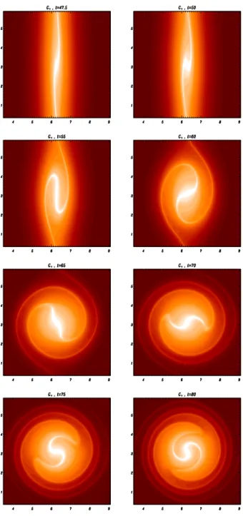
The advection of the two Lagrangian invariantsG±is de-termined by the stream functionsϕ±. The winding, caused by this differential rotation type of advection makesG± in-creasingly filamented inside the magnetic island, leading to a mixing process. These filamentary structures of G± do not influence the spatial structure ofψwhich remains regu-lar. The advection of the Lagrangian invariants is shown in Fig. 1 where we draw the shaded isocontours ofG+at time
Fig. 1. Shaded isocontours of the Lagrangian invariantG+in the central region of the (x,y) domain of integration. The frames are obtained at timest=47.5,50,55,60,65,70,75,80 for a run with
̺s/de=1.5,Lx=4π,Ly=21pi.
t=47.5, 50, 55, 60, 65, 70, 75, 80 for a run with̺s/de=1.5.
of small scales, while the divergence free advection veloci-ties derived from the stream functionsϕ± must necessarily stretch the plasma in order to preserve areas.
4.4 Onset of a secondary Kelvin Helmholtz instability: tur-bulent versus laminar mixing
The advection, and consequently the mixing, of the La-grangian invariants can be either laminar or turbulent de-pending on the value of̺s/de. The transition between these
two regimes was shown in Del Sarto et al. (2003). to be related to the onset of a secondary Kelvin Helmholtz-type (K-H) instability driven by the velocity shear of the plasma motions that form because of the development of the recon-nection instability. Whether or not the K-H instability be-comes active before the island growth saturates, affects the redistribution of the magnetic energy and determines whether a (macroscopically) stationary reconnected configuration is reached.
In the cold electron limit,̺s/de=0, the system of Eqs. (17)
becomes degenerate and the generalized connections are de-termined by a single Lagrangian invariantF. Initially, F
is advected along a hyperbolic pattern given by the stream functionϕ which has a stagnation point at theO-point of the magnetic island. This motion leads to the stretching of the contour lines ofF towards the stagnation point and to the formation of a bar-shaped current layer along the equilib-rium null line, which differs from the cross shaped structure found in the initial phase of the reconnection instability for
̺s/de6=0. Subsequently,F contours are advected outwards in
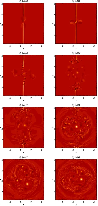
thex-direction. At this stageF starts to be affected by a K-H instability that causes a full redistribution ofF. In this phase the spatial structure ofF is dominated by the twisted fila-ments of the current density which spread through the central part of the magnetic island. The evolution of the Lagrangian invariantF is shown in Fig. 2 where its shaded isocontours are plotted at timest=100, 102, 106, 111, 117, 127, 137, 147 in the central region of the (x,y) domain of integration.
After the onset of the secondary instability the contours of the vorticityU, see Fig. 3, exhibit a well developed turbulent distribution of monopolar and dipolar vortices, while those ofψremain regular although they pulsate in time. The en-ergy balance shows that part of the released magnetic enen-ergy remains in the form of plasma kinetic energy corresponding to the fluid vortices in the magnetic island and that an oscilla-tory exchange of energy persists between the plasma kinetic energy and the electron kinetic energy (see also Bergmans et al., 1998) corresponding to the pulsations of the island shape.
This turbulent evolution of the nonlinear reconnection pro-cess persists in the non degenerate, finite electron temper-ature, case where the two Lagrangian invariantsG± deter-mine the generalized linking conditions However, as the ratio
̺s/deis increased, i.e. as the electron temperature effects
be-come more important, the onset of the K-H instability occurs later during the island growth and its effect on the current layer distribution becomes weaker. For̺s/de∼1, no sign of
Fig. 2.Shaded isocontours of the Lagrangian invariantFin the cen-tral region of the (x,y) domain of integration. The frames are ob-tained at timest=100,102,106,111,117,127,137,147 for a run with̺s=0,Lx=4π,Ly=21pi.
a secondary instability is detectable during the time the island takes to saturate its growth.
In the transitional regime, the advection pattern and the current layer structures exhibit an intermediate behaviour. Initially,G±are advected in opposite directions with a dif-ferential rotation, as is the case for̺s/de=1. At later times
they acquire features characteristic of the evolution ofF in the degenerate̺s=0 case and their advection becomes K-H
Fig. 3. Shaded isocontours of the vorticityUin the central region of the (x,y) domain of integration. The frames are obtained at times
t=100,102,106,111,117,127,137,147 for the same run of Fig. 2.
4.5 Need for a kinetic electron description
The above results show that the conservation of the general-ized connections in the reconnection process leads to the for-mation of current and vorticity layers with spatial scales that, in the absence of dissipation, becomes increasingly small with time. In this nonlinear phase of the development of the reconnection instability, in the presence of thermal ef-fects, the fluid approximation becomes inconsistent inside
the layers. The generalized connections and the constraints that they exert on the plasma dynamics apply to the case of a fluid plasma, where fluid elements can be defined and the linking property between fluid plasma elements can be for-mulated.
It thus becomes important to understand what is the role of the topological invariants in a kinetic electron description where e.g., the canonical momenta of the single electrons do not simply add up to give the fluid conserved Lagrangian invariant F discussed above. The role of a finite electron temperature on the topological properties of the plasma is al-ready evident from the above results, since the contribution of the parallel electron compressibility introduces two new Lagrangian invariantsG±and two different streaming func-tionsϕ±instead ofF andϕ, and consequently changes the nonlinear evolution of reconnection in a significant way.
5 Drift kinetic formulation
Let F(x, y, v||, t ) be the drift-kinetic electron distribution function, withv||the electron velocity coordinate along field lines. It is convenient to adopt the electron canonical mo-mentum, divided by the electron mass,p||, defined by2
p|| ≡v||−ψ , (20)
as the kinetic variable instead ofv||. Since we consider two dimensional (z independent) fields and perturbations,p||is a particle constant of the motion.
In thex, y, p||, tvariables the drift kinetic equation for the distribution functionf (x, y, p||, t )≡F(x, y, v||, t )reads (de Blank, 2001; Valori, 2001; de Blank et al., 2003)
∂f
∂t + [ϕ−ψp||−ψ 2/
2, f] =0− [ϕkin, f], (21)
withϕkin=ϕ−ψp||/c−ψ2/2.Note that in Eq. (21) the spa-tial derivatives are taken at constantp|| and not at constant
v||. For each fixed value ofp||, the time evolution off corre-sponds to that of a Lagrangian invariant “density” advected by the velocity field obtained from the generalized stream functionϕkin.
The advection velocity field is different on eachp||=const foil. Thus, as noted in Liseikina et al. (2004), f consists of an infinite number of Lagrangian invariants, each of them advected with a different velocity, that take the place of the two fluid invariantsG±in Eqs. (17).
The fluid quantities are defined in terms of distribution functionf as follows
Z
dp||f (x, y, p||, t )n(x, y, t ) ,
Z
dp||p||f (x, y, p||, t )[u(x, y, t )−ψ (x, y, t )]n(x, y, t ) ,
2We adopt the following normalizations ϕ=eϕ/m
evt he2 , ψ=eψ/mecvt he,x, y=x/L,y/L,t=t mev2t hec/L2eB0,p||=
p||/vt he, whereLis a characteristic length and the other symbols
Z
dp||[p||−u(x, y, t )+ψ (x, y, t )]2f (p||, x, y, t )5||||, (22) where n(x, y, t ) andu(x, y, t )are the normalized electron density and fluid velocity and5||||(x, y, t )is the(z, z) com-ponent of the pressure tensor. Then Ampere’s equation reads
de2∇2ψ=nu, (23)
and, as in the fluid case, the ion equation of motion together with quasineutrality give
(n−n0)=ρs2∇2ϕ, (24)
wheren0 = n0(x)is the initial normalized density and the
density variations are supposed to remain small.
The above system of equations admits a conserved energy functionalHkin
Hkin= Z d2x
2 [d
2
e(∇ψ )2+ρs2(∇ϕ)2+nu2+5||||] (25) Aside for the normalization, the main difference between these energy terms and the corresponding ones derived in the fluid case, see Eq. (19), is in the expression of the electron compression work, as natural in a kinetic theory, the pres-sure tensor5|||| cannot be expressed in terms of the lower order moments of the distribution function.
5.1 Electron equilibrium distribution function
The stationary solutions of Eq. (21) are of the form
f=f (p||, ϕkin).Using the identity for the single particle
en-ergy
v||2/2−ϕ=p||2/2−ϕkin, (26)
we can write a stationary distribution function that depends only on the particle energy asf=f (p||2/2−ϕkin), while the
well known static (ϕ0=0) Harris pinch equilibrium
distribu-tion (Harris (1962)) is given by3
f =f0exp[−(p||2−2ϕkin)−2v∗p||] (27) In order to have a less inhomogeneous plasma configura-tion we can add a pedestal (Maxwellian) distribuconfigura-tion func-tion of the form fped=f00exp[−(p2||−2ϕkin)]. The
corre-sponding self consistent vector potentialψ0(x)is given by ψ0(x)=(1/v∗)ln(coshx) and the shear magnetic field has
the standard hyperbolic tangent distribution. 5.2 Evolution of thep||=const foils
We write the distribution function with f (x, y, t, p||) as
f (x, y, t, p||)=R dp¯||δ(p¯||−p||)f (x, y, t,p¯||). This is a fo-liation of the electron distribution function in terms of the in-finite number of Lagrangian invariants obtained by taking the
3In velocity variable v
|| this distribution corresponds to F0exp[−(v||−v∗)2−2v∗ψ]and leads to a particle and current den-sity of the formn=n0exp(−2v∗ψ)andj=−n0v∗exp(−2v∗ψ), wherejis normalized onnoevt heandv∗is the standard parameter
related to the diamagnetic fluid motion.
distribution functionf at fixed electron canonical momen-tum. Within the drift-kinetic equation eachp¯||-foil evolves independently, while all foils are coupled through Maxwell’s equations. The total number of particles in each foil is con-stant in time.
In the initial configuration, the spatial dependence of each p¯||-foil is given for the case of the Harris distribu-tion by exp(2ϕ¯kin)=exp(−2ψp¯||−ψ2)=exp[ ¯p||2− ˆv||(x)2], wherevˆ||(x)≡v||(ψ,p¯||)= ¯p||+(1/v∗)ln(coshx). For nega-tive values ofp¯||the maximum of the argument of the expo-nent is located atx=±arccosh[exp(−v∗p¯||)]i.e. the foil is localized in space within two symmetric bands, respectively to the right and to the left of the neutral line of the magnetic configuration. For positive values ofp¯||all the foils are cen-tered aroundx=0.
5.3 Nonlinear twist dynamics of the foils
In the adopted drift kinetic framework thep¯||-foils take the role of the Lagrange invariantsG± of the fluid plasma de-scription. In this perspective, the dynamics of the foils can be predicted by looking at the form of stream functionϕkin
inside each foil. The advection velocity can be written as ez×∇(ϕ−ψp||−ψ2/2)=ez×∇ϕ+(p||+ψ )∇ψ×ez, (28)
which represents the particleE×Bdrift and their free motion along field lines.
At fixed p||= ¯p|| we see that depending on the sign of
ψ+ ¯p||= ˆv||(x), the advection velocity field takes two counter oriented rotation patterns, reminiscent of those that advect
G− (G+) in fluid theory. In the equilibrium configura-tion where all quantities are funcconfigura-tion ofψ=ψ (x)andϕ=0, this advection corresponds to the free particle motion along
ψ=const surfaces inside each foil. However, when the in-stability starts to move the plasma along the x axis and
∂ϕ/∂y6=0, the portions of the foil wherevˆ||>0 or wherevˆ||<0 bend in opposite directions. This leads to a distortion and twist of the foils and to their eventual spatial mixing, analo-gously to the mixing ofG±in fluid theory.
6 Numerical results: drift-kinetic regime
For a Harris equilibrium the evolution of the reconnection in-stability is characterized by three dimensionless parameters that can be expressed as the dimensionless ion sound gyro-radiusρs and the electron skin depthdefrom Poisson’s and
Ampere’s equations respectively, andn0. In fact, whende
andn0are given,v∗, and thusψ0, are determined implicitly
by the choice ofL.
The size of the simulation box along y has been cho-sen equal to 4π such that the parameter1′is positive only for the lowest order mode corresponding toky=1/2 so that
only theky=1/2 mode can be linearly unstable. The
as foli- infi-the momen-es s
con-each by
,
or the the re-the foils
the de-can
(28)
mo-counter ect configuration , along the and where distortion mixing,
in--3 0 3 -4
0 4
y
0.05
0.10
0.15
0.20
0.25
-3 0 3 -4
0 4
Y
X
-3 0 3 -4
0 4
y
0.41
0.45
0.49
0.53
-3 0 3 -4
0 4
Y
X
-3
0
3
-4
0
4
Y
X
-3
0
3
-4
0
4
X
Y
Fig. 4. Contour plots (top) and 3-D plots (middle) of the
p||=constant foils of electron distribution function and contour plots (bottom) of the kinetic stream function ϕkin at t=81 for p||=−1.5,−0.5 from left to right in the interval−4<x<4 around the neutral line. Note the different scales in the vertical axes of the 3-D plots.
to ψ0=1/4, n0=1/16, de=1, v∗=2(=>ψ0=1/2, n0=1/4), de=0.5, v∗=2(=>ψ0=1/2, n0=1/16). Smaller values ofv∗
correspond to larger instability growth rates i.e., to faster evolving instabilities where the saturation of the island
-3 0x 3 -4
0 4
y
0.08 0.25 0.42
-3 0 3 -4
0 4
Y
X
-3 0x 3 -4
0 4
y
0.00 0.02 0.04 0.06
-3 0 3 -4
0 4
Y
X
-3
0
3
-4
0
4
X
Y
-3
0
3
-4
0
4
X
Y
Fig. 5. Contour plots (top) and 3-D plots (middle) of the
p||=constant foils of the electron distribution function and con-tour plots (bottom) of the kinetic stream functionϕkinatt=81 for p||=0.5,1.5 from left to right in the interval−4<x<4 around the neutral line. Note the different scales in the vertical axes of the 3-D plots.
growth is reached sooner. Here we present the results ob-tained in the case with de=1 and v∗=4. The evolution of
in Fig. (4) and forp¯||=0.5,1.5 in Fig. (5), together with the contour plots of the stream functionϕkinin x−y for the same
values ofp¯||and the same interval in x.
Foils corresponding to negative values ofp¯||were initially localized in two symmetric bands to the left and to the right of the neutral line and are thus modified by the onset of the reconnection instability only in their portion that extend into the reconnection region. On the contrary foils corresponding to positive values ofp¯|| were initially localized around x=0 and are thus twisted by the development of the reconnection instability. The contour plots of the stream functionϕkin
cor-responds to a differential rotation in the x−y plane. The sign of the rotation is opposite for positive and for negative values ofp¯||. The mixing caused by this differential rotation of the
p||-foils is evident. As in the fluid case, the mixing of the Langrangian invariants in x−y space is accompanied by the energy transfer towards increasingly small scales.
Within the range of parameters explored in the simulations discussed in the present paper, we have not evidenced any onset of a secondary instability. This result is fully consis-tent with the fluid simulations that show that the onset of the Kelvin-Helmholtz instability is impeded by increasing the electron temperature.
In summary, the Lagrangian invariants obtained by writ-ing the drift-kinetic electron distribution function as a foli-ation of an infinite number of fluid type distributions taken at fixed parallel canonical momentum, lead us to establish a clear link between the fluid and the kinetic regimes of the re-connection instability since the (two) fluid invariants and the (infinite) drift-kinetic invariants evolve in time in an analo-gous fashion. In both cases the mixing of the Langrangian invariants in x-y space and the energy transfer towards in-creasingly small scales make it possible for the system to reach a different macroscopic magnetic equilibrium with a saturated magnetic island and with a lower magnetic energy even in the absence of dissipation.
7 Conclusions
Magnetic field line reconnection in collisionless system is controlled by topological constraints that evolve in very sim-ilar forms in fluid and in kinetic regimes.
The form of these topological constraints depends explic-itly on the microscopic physics that governs the reconnection process in the plasma. We find that the value of the micro-scopic parameters, such as the electron skin depthdeand the
ion sound gyro-radius̺s in the fluid regimes, and the
cor-responding parameters in the drift kinetic regime, determine not only the linear growth rates of the reconnection instabil-ities, but also their characteristic nonlinear evolution times and, most important, the spatial distribution of the current and vorticity layers produced during the nonlinear develop-ment of the instabilities.
Indeed we find that, in the fluid regime, the ratio̺s/de
de-termines a transition between a turbulent nonlinear regime, where long lasting fluid vortices develop inside a pulsating
magnetic island, and a laminar regime with a (macroscopi-cally) stationary island. In both regimes the current and vor-ticity layers eventually fill the entire magnetic island.
The topological constraints play an important role also in the kinetic regimes, as we have shown in the case of the drift kinetic model of the electron response for a two dimensional magnetic configuration with a strong guide field. In particu-lar we have shown that the mixing of the Lagrangian invari-ants, the formation of smaller and smaller spatial scales and the energy transfer towards these increasingly small scales is common to the fluid and to the kinetic regimes of the Hamiltonian dynamics of a collisionless plasma and can be described in both regimes in analogous mathematical terms. Acknowledgements. Part of this work was supported by the INFM Parallel Computing Initiative and by the Italian Ministry for University, by Scientific Research PRIN 2002 funds, by Russian Science Support Foundation and by Russian Foundation for Basic Research (Grant 04-01-00850).
Edited by: P.-L. Sulem Reviewed by: two referees
References
Bhattacharjee, A., Ma, Z. W., Wang, X.: Recent developments in collisionless reconnection theory: Applications to laboratory, space plasmas,Phys. Plasmas, 8, 1829–1839, 2001.
Bergmans, J. and Schep, T. J.: Merging of Plasma Currents, Phys. Rev. Lett., 87, 195002–+, 2001.
Brunetti, M., Califano, F., and Pegoraro, F.: Asymptotic evolu-tion of nonlinear Landau damping, Phys. Rev. E, 62, 4109–4114, 2000.
Cafaro, E., Grasso, D., Pegoraro, F., Porcelli, F., and Saluzzi, A.: Invariants, Geometric Structures in Nonlinear Hamiltonian Mag-netic Reconnection, Phys. Rev. Lett.,, 80, 4430–4433, 1998. de Blank, H. J.: Kinetic model of electrons in drift-Alfv´en
current-vortices, Physics of Plasmas, 8, 3927–3935, 2001.
de Blank, H. J. and Valori, G.: Electron kinetics in collisionless magnetic reconnection, Plasma Physics, Controlled Fusion, 45, A309–A324, 2003.
Del Sarto, D. Califano, F., and Pegoraro, F.: Secondary instabilities and vortex formation in collisionless-fluid magnetic reconnec-tion, Phys. Rev. Lett., 91, 235001–+, 2003.
Fitzpatrick, R.: Scaling of forced magnetic reconnection in the Hall-magnetohydrodynamic Taylor problem, Phys. Plasmas, 11, 937– 946, 2004.
Fitzpatrick, R.: Scaling of forced magnetic reconnection in the Hall-magnetohydrodynamical Taylor problem with arbitrary guide field, Phys. Plasmas, 11, 3961–3968, 2004.
Grasso, D., Califano, F., and Pegoraro, F.: Ion Larmor Radius Ef-fects in Collisionless Reconnection, Plasma Phys. Rep., 26, 512– 518, 2000.
Grasso, D., Califano, F., Pegoraro, F., and Porcelli, F.: Phase Mix-ing, Island Saturation in Hamiltonian Reconnection, Phys. Rev. Lett.,, 86, 5051–5054, 2001.
Kuvshinov, B. N., Pegoraro, F., and Schep, T. J.: Hamiltonian for-mulation of low-frequency, nonlinear plasma dynamics,Physics Letters A, 191, 296–300, 1994.
Kuvshinov, B. N., Lakhin, V. P., Pegoraro, F., and Schep, T. J.: Hamiltonian vortices and reconnection in a magnetized plasma, J. Plasma Physics, 59, 727–736, 1998.
Lancellotti, C., Dorning, J. J.: Nonlinear Landau Damping in a Col-lisionless Plasma, Phys. Rev. Lett., 80, 5236–+, 1998.
Lancellotti, C., Dorning, J. J.:Time-asymptotic wave propagation in collisionless plasmas, Phys. Rev. E, 68, 026406–+, 2003. Liseikina, T. V., Pegoraro, F., and Echkina, E. Yu.: Phys. Plasmas,
11, 3535–3545, 2004.
Manfredi, G.: Long-Time Behavior of Nonlinear Landau Damping, Phys. Rev. Lett., 79, 2815–2818, 1997.
Morrison, P. J.: Hamiltonian formulation of reduced magnetohy-drodynamics, Phys. Fluids, 27, 886–897, 1984.
Ottaviani, M. and Porcelli, F.: Nonlinear collisionless magnetic re-connection, Phys. Rev. Lett., 71, 3802–3805, 1993.
Ottaviani, M. and Porcelli, F.: Fast nonlinear magnetic reconnec-tion, Phys. Plasmas, 2, 4104–4117, 1995.
Pegoraro, F.: Magnetic Field Line Reconnection in Dissipa-tionless Regimes and Mixing of the Lagrangian Invariants in Strongly Magnetized, Two-dimensional, Plasma Configurations, in: Thematic Program in Partial Differential Equations, Work-shop on Kinetic Theory, Fields Institute Toronto, http://www. fields.utoronto.ca/audio/\#kinetic/, 2004.
Porcelli, F., Borgogno, D., Califano, F., Grasso, D., Ottaviani, M., and Pegoraro, F.: Recent advances in collisionless magnetic re-connection, Plasma Phys. Contr. Fusion, 44, B389 405, 2002. Rogers, B. N., Denton, R. E., Drake, J. F., and Shay, M. A.: Role of
Dispersive Waves in Collisionless Magnetic Reconnection, Phys. Rev. Lett., 87, 195004–+, 2001.
Schep, T. J., Pegoraro, F., and Kuvshinov, B. N.: Generalized two-fluid theory of nonlinear magnetic structures, Physics of Plasmas, 1, 2843–2852, 1994.
Shay, M. A., Drake, J. F., Swisdak, M., and Rogers, B. N.: The scaling of embedded collisionless reconnection, Phys. Plasmas, 11, 2199–2213, 2004.
Valori, G.: Fluid, kinetic aspects of collisionless magnetic recon-nection, ISBN 90-9015313-6, Print Partners Ipskamp, Enschede, the Netherlands, 2001.