www.nonlin-processes-geophys.net/21/645/2014/ doi:10.5194/npg-21-645-2014
© Author(s) 2014. CC Attribution 3.0 License.
A note on Taylor’s hypothesis under large-scale flow variation
M. Wilczek1, H. Xu2, and Y. Narita3,4
1Department of Mechanical Engineering, The Johns Hopkins University, 3400 North Charles Street, Baltimore, MD 21218, USA
2Max Planck Institute for Dynamics and Self-Organization (MPIDS), Am Fassberg 17, 37077 Göttingen, Germany 3Space Research Institute, Austrian Academy of Sciences, Schmiedlstr. 6, 8042 Graz, Austria
4Institut für Geophysik und extraterrestrische Physik, Technische Universität Braunschweig, Mendelssohnstr. 3, 38106 Braunschweig, Germany
Correspondence to:M. Wilczek ([email protected])
Received: 16 December 2013 – Revised: 17 March 2014 – Accepted: 16 April 2014 – Published: 2 June 2014
Abstract. Experimental investigations of turbulent velocity fields often invoke Taylor’s hypothesis (also known as frozen turbulence approximation) to evaluate the spatial structure based on time-resolved single-point measurements. A cru-cial condition for the validity of this approximation is that the turbulent fluctuations are small compared to the mean veloc-ity, in other words, that the turbulence intensity must be low. While turbulence intensity is a well-controlled parameter in laboratory flows, this is not the case in many geo- and astro-physical settings. Here we explore the validity of Taylor’s hypothesis based on a simple model for the wavenumber-frequency spectrum that has recently been introduced as a generalization of Kraichnan’s random sweeping hypothesis. In this model, the fluctuating velocity is decomposed into a large-scale random sweeping velocity and small-scale fluc-tuations, which allows for a precise quantification of the in-fluence of large-scale flow variations. For turbulence with a power-law energy spectrum, we find that the wavenum-ber spectrum estimated by Taylor’s hypothesis exhibits the same power-law as the true spectrum, yet the spectral energy is overestimated due to the large-scale flow variation. The magnitude of this effect, and specifically its impact on the experimental determination of the Kolmogorov constant, are estimated for typical turbulence intensities of laboratory and geophysical flows.
1 Introduction
One of the central results from Kolmogorov’s celebrated phe-nomenology (Kolmogorov, 1941) is that the turbulence en-ergy spectrum function takes the form
E(k)=CKε2/3k−5/3 (1) in the inertial range of scales, that is, the range of scales which is clearly separated from the large, energy-containing scales and the small, dissipative scales. Hereεis the mean rate of energy dissipation and CK is often called the Kol-mogorov constant. The energy spectrum (Eq. 1) and its one-dimensional counterparts have been observed in many labo-ratory, atmospheric and oceanic flows. Consequently, there is a strong theoretical and practical interest in determin-ing the value of CK, which is assumed to be a universal constant, especially from atmospheric turbulence data (see, e.g., Sreenivasan, 1995).
calibration and maintenance. For intrusive techniques such as HWA, installing many probes in the flow could even re-sult in large disturbances that render the measurements in-valid. Moreover, optical-based techniques (PIV and LDV) re-quire uniformly seeded tracer particles for best performance, which is difficult to achieve in geophysical flow measure-ments. Recent advances in remote sensing provide valuable data on large-scale mean flow fields. The spatial resolutions of these data, however, are still too low to allow quantitative measurement of the energy spectra. Therefore, to date, the energy spectra of geophysical flows are almost exclusively measured with a single probe, and Taylor’s frozen turbulence hypothesis is used to reconstruct the spatial variation of the velocity field, which assumes that turbulent fluctuations are carried with the mean flow in a quasi-frozen manner (Taylor, 1938). In other words, instead of spatial variations, experi-ments usually measure temporal signals that are then mapped to the spatial domain. For the energy spectrum this means that the frequencyωis related to the streamwise wavenum-berkzby the simple relationω=kzU, whereU is the mean
velocity of the flow.
The validity of this approximation has widely been stud-ied in various geophysical field and laboratory experiments; some examples include oceanic and surface-water turbulence (MacMahan et al., 2012), atmospheric turbulence (Lappe and Davidson, 1963; Mizuno and Panofsky, 1975; Castro et al., 2011), precipitation field distributions in meteorology (Li et al., 2009), wall turbulence (Uddin et al., 1997), and wind tunnel experiments (LeBoeuf and Mehta, 1995).
Taylor’s hypothesis is limited by the fact that the turbulent fluctuations also evolve in time, which means they usually cannot be regarded as frozen-in. This limitation becomes es-pecially apparent when the turbulent fluctuations are compa-rable to the mean flow, such as at high turbulence intensities. Moreover, the fluctuations of the velocity field contain large-scale variations, sometimes termed random sweeping veloc-ity (Kraichnan, 1964; Tennekes, 1975), which are difficult to discriminate from the mean velocity due to their large-scale nature. The aim of this paper is to focus on the latter effect and to quantify the influence of these large-scale flow vari-ations on the energy spectrum as it is usually measured in experiments.
This idea has been discussed in prior literature, for ex-ample by Lumley (1965) who studied the effects of ran-dom sweeping by keeping only the first two terms in the series expansion of the characteristic function of the large-scale velocity fluctuations. His work later was picked up by Wyngaard and Clifford (1977) and compared to the case of a Gaussian large-scale random sweeping velocity. They found that the Gaussian random sweeping assumption agrees well with Lumley’s two-term expansion for low to moder-ate turbulence intensities. Based on their model calculations they were able to show that random sweeping effects lead to systematic deviations in many statistical quantities inferred
from single-point measurements using Taylor’s hypothesis, including the spectral energy levels.
In this note, we make use of a simple theoretical model recently introduced for the wavenumber-frequency spectrum by Wilczek and Narita (2012). This model spectrum can be regarded as the result of a generalized Taylor’s hypothesis, which takes into account the advection of turbulent fluctua-tions not only by a mean flow, but also by a random large-scale velocity field and is essentially based on Kraichnan’s ideas of random sweeping (Kraichnan, 1964). Based on the same mathematical approach also used by Wyngaard and Clifford for their model calculations, our results are in line with their findings. Here, we will however focus the discus-sion on the impact of large-scale random sweeping on the determination of the Kolmogorov constant. In particular, we obtain a closed-form analytical expression that quantifies the effect of large-scale random sweeping on the Kolmogorov constant determined using Taylor’s hypothesis.
The procedure is the following: given an energy spec-trum function in wavenumber space, our theoretical model makes an estimate for the wavenumber-frequency spectrum parametrized by the mean and the sweeping velocity. This wavenumber-frequency spectrum serves as an “ideal” refer-ence spectrum, which then can be reduced to the frequency spectrum. In the next step, Taylor’s hypothesis, as used in ex-periments, is applied to the frequency spectrum to obtain an expression for the energy spectrum function in wavenumber space, here called the Taylor spectrum. By comparing this ap-proximate spectrum to the “true” Kolmogorov energy spec-trum function, the influence of large-scale flow variations can be systematically tested. It especially allows discussing cor-rections to the experimental measurement of the Kolmogorov constant due to random sweeping effects.
2 Wavenumber-frequency spectrum
As detailed in Wilczek and Narita (2012), we make a num-ber of simplifying assumptions to obtain an analytical model for the wavenumber-frequency spectrum. We assume that the large-scale random sweeping velocity and the small-scale ve-locity fluctuations are statistically independent initially. Fur-thermore, we assume the random advection to be isotropic and Gaussian distributed and the small scales to be isotropic with a given energy spectrum function. We then essentially consider a linear advection problem in which the turbulent fluctuations are advected by a mean velocityU (assumed in
is a product of a wavenumber spectrum with a Gaussian fre-quency distribution:
E(k, ω)dkdω= E(k)
4π k2√2π k2V2 exp
"
−(ω−kzU )
2
2k2V2 #
dkdω. (2)
Here, E(k) is the energy spectrum function of the small-scale velocity fluctuations. In the following, we will re-strict ourselves to a power-law spectrum, which follows Kolmogorov’s phenomenology, cf. Eq. (1). The mean of the Gaussian distribution kzU describes the Doppler shift,
whereas the standard deviation k V describes the Doppler broadening. Note that both effects become more important with increasing wavenumbers.
It is worthwhile to note that in the limit of vanishing sweeping velocity, Taylor’s hypothesis again becomes valid. This can be seen by
lim
V→0E(
k, ω)dkdω= E(k)
4π k2δ (ω−kzU )dkdω, (3) where the delta function simply indicates that the frequency can be relabeled with the streamwise wavenumber. As the standard deviation of the Gaussian distribution of the model spectrum is k V, the rate of convergence to a delta function decreases with increasingk.
By integrating the model (Eq. 2) over the wave vector do-main, the energy in the frequency domain can be obtained as (Wilczek and Narita, 2012)
E(ω)dω=CF(U, V ) CKε2/3ω−5/3dω, (4) whereCFdenotes the coefficient
CF(U, V )=
∞ Z
0 dx
erf
x +U √
2V
−erf x
−U √
2V
x2/3
2U. (5) Here we have assumed an infinitely extended inertial range. Note that while the frequencyωin Eq. (2) can take both pos-itive and negative values, we consider only pospos-itive frequen-cies in Eq. (4) since positive and negative frequenfrequen-cies can-not be discriminated by a single-point measurement. Con-sequently, a factor of two is included into Eq. (5) in order to conserve the total energy. Given an Eulerian wavenum-ber spectrum with index−5/3, also the Eulerian frequency spectrum will exhibit this power-law index, independent of mean flow and sweeping velocity. The prefactor, how-ever, depends on U andV. This implies that the observa-tion of a frequency spectrum consistent with Kolmogorov’s phenomenology does not guarantee the validity of Taylor’s hypothesis.
3 Implications for the measurement of the Kolmogorov constant
We now come to the main part of this paper and discuss the implications of our model on the measurement of the Kol-mogorov constant. To this end, we derive an expression for the energy spectrum function obtained with the help of Tay-lor’s hypothesis. This will be referred to as the Taylor energy spectrum function, which then can be compared to the Kol-mogorov energy spectrum function. We start by stressing that the quantityE(ω)dωrepresents the energy contained in an infinitesimal frequency interval dω. This quantity is exper-imentally accessible by measuring time series of all veloc-ity components, for example by anemometry with an X-wire configuration. To apply Taylor’s hypothesis, the frequency is simply related to the wavenumber in the streamwise direction byω=kzU, which upon insertion into Eq. (4) leads to
e
E (kz)dkz=E(ω)
dω
dkz
dkz
=CF(U, V ) U−2/3CKε2/3k−z5/3dkz. (6)
This spectrum describes the energy density of the turbu-lent fluctuations resolved with respect to the streamwise wavenumberkz and thus is related to the one-dimensional
spectra (Pope, 2000)
Eij(kz)=
1
π
∞ Z
−∞
dzui(x) uj(x+zez)
exp−i kzz
(7)
by e
E (kz)=
1
2Eii(kz) . (8)
For power-law spectra of Kolmogorov type, as considered here, a simple relation between the one-dimensional spectra and the energy spectrum function exists in the inertial range (Pope, 2000),
1
2Eii(k)= 3
5E(k). (9)
Together with Eq. (6), this leads to the Taylor energy spec-trum function:
ET(k)=CT(U, V ) CKε2/3k−5/3 (10) with
CT(U, V )= 5 3U
−2/3C
The interesting point about this result is that the energy spectrum measured with Taylor’s hypothesis takes the form of the original Kolmogorov energy spectrum function (Eq. 1) multiplied by a factor that depends on the mean and random sweeping velocities.CT(U, V )is a non-dimensional prefac-tor that depends only on the ratioξ=V /U.ξ can be iden-tified with the turbulence intensity in good approximation, because the kinetic energy in the small-scale velocity field is small compared to the fluctuations of the random sweeping field. To explicitly see that, we substitute Eq. (5) into Eq. (11) and obtain
CT(ξ )= 5 6
∞ Z
0 dy
erf
y
+1
√
2ξ
−erf y
−1
√
2ξ
y2/3. (12)
This result stresses the importance of the turbulence inten-sity for the validity of Taylor’s hypothesis. In the limit of vanishing turbulence intensity (corresponding toξ→0) the “true” Kolmogorov energy spectrum function has to be covered. In this case the error functions in the integrand re-duce to sharp Heaviside cutoffs, which leads to
lim
ξ→0CT(ξ )= 5 3
1 Z
0
dy y2/3 =1. (13)
For non-vanishing turbulence intensities, however, these cut-offs are smoothed out. A closer inspection of the expression shows that CT≥1. This can be seen by appreciating that the error-function term represents a bump-shaped function which preserves its area irrespective of the turbulence inten-sity. Compared to the zero-turbulence intensity case, the am-plitude of the bump is decreased fory <1, but almost sym-metrically we now get contributions fory >1. As this error function term in the integrand is weighed by the monoton-ically increasingy2/3, the correction has to be positive and increasing with the turbulence intensity.
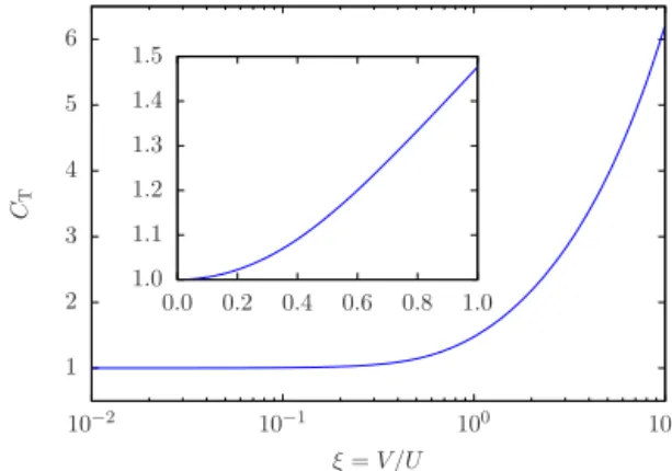
A graphical evaluation of the coefficientCTas a function of turbulence intensity is presented in Fig. 1. It is evident that the influence for moderate turbulence intensities below 25 %, as they are usually met in experimental setups, is quite small. For example, in conventional passive grid turbulence in a wind tunnel, the turbulence intensityξis typically below 5 %. Hence the correction to CK expected from our theory is negligible. In more recent active grid turbulence in a wind tunnel, the turbulence intensity is usually below 20 %, which leads to corrections of around 2 % or less. For turbulent jets,
ξ in the centerline can reach about 25 %. Even in this case the correction toCKis still small, approximately 3.5 % only. If, however, the large-scale fluctuations exceed the mean flow, significant errors occur.
As summarized in Sreenivasan (1995), experimentally measured CK for 50< Rλ/2×104 lie within the range
1.62±0.17. These values are in general agreement with DNS results, but the scatter of data is significant. Sreenivasan
1 2 3 4 5 6
10−2 10−1 100 101
CT
ξ=V /U 1.0
1.1 1.2 1.3 1.4 1.5
0.0 0.2 0.4 0.6 0.8 1.0
Figure 1.CoefficientCTof the Taylor spectrum (Eq. 10) as a
func-tion of the (approximate) turbulence intensityξ=VU.
(1995) argued that neither the stability nor the large-scale shear in the atmospheric surface layer caused large varia-tions ofCK; each of the two mechanisms affectsCK by a few percent. The results discussed here, in line with those of Wyngaard and Clifford, provide an additional source which adds to the experimental scatter in measuredCK values in geophysical flows, which are featured with strong fluctua-tions at large scales.
It would also be interesting to extend our analysis to plasma turbulence, in which a −5/3 spectrum in the fre-quency domain has been reported by various in situ space-craft observations of the magnetic field in solar wind tur-bulence, for example, ranging over nearly three orders of magnitude as measured by the WIND spacecraft (Podesta et al., 2007). Naively speaking, the use of Taylor’s hypoth-esis seems to be justified in this case since the fluctuation of the flow velocity is of the order of 10 % of the mean flow (about 400 km s−1). However, the magnetic field fluctuation may reach 100 % of the mean field (which is in the range 1 to 10 nT). Thus the effect of the Alfvén waves needs to be in-cluded for a quantitative estimate of Taylor’s hypothesis in the solar wind.
4 Conclusions
turbulence intensities can reach high levels where significant corrections to the measurement have to be taken into account.
Acknowledgements. M. Wilczek acknowledges funding by
DFG WI 3544/2-1. H. Xu gratefully acknowledges partial support from DFG through project A7 in SFB 963 AstroFIT. The work is also supported by FP7 313038/STORM.
Edited by: B. Tsurutani
Reviewed by: O. Verkhoglyadova and another anonymous referee
References
Li, B., Murthi, A., Bowman, K. P., North, G. R., Genton, M. G., and Sherman, M.: Statistical tests of Taylor’s hypothesis: an intro-duction to precipitation fields, J. Hydrometeorol., 10, 254–265, 2009.
Castro, J. J., Carsteanu, A. A., and Fuentes, J. D.: On the phe-nomenology underlying Taylor’s hypothesis in atmospheric tur-bulence, Revista Mexicana de Física, 57, 60–64, 2011.
Kolmogorov, A. N.: The local structure of turbulence in incom-pressible viscous fluid for very large Reynolds number, Dokl. Akad. Nauk. SSSR, 30, 299–303, 1941.
Kraichnan, R. H.: Kolmogorov’s hypothesis and Eulerian turbu-lence theory, Phys. Fluids, 7, 1723–1734, 1964.
Lappe, U. O. and Davidson, B.: On the range of validity of Taylor’s hypothesis and the Kolmogoroff spectral law, J. Atmos. Sci., 20, 569–576, 1963.
LeBoeuf, R. L. and Mehta, R. D.: On using Taylor’s hypothesis for three-dimensional mixing layers, Phys. Fluids, 7, 1516–1518, 1995.
Lumley, J. L.: Interpretation of time spectra measured in high-intensity shear flows, Phys. Fluids, 8, 1056–1062, 1965. MacMahan, J., Reniers, A., Ashley, W., and Thornton, E.:
Frequency-wavenumber velocity spectra, Taylor’s hypothesis, and length scales in a natural gravel bed river, Water Resource Res., 48, W09548, doi:10.1029/2011WR011709, 2012. Mizuno, T. and Panofsky, H. A.: The validity of Taylor’s hypothesis
in the atmospheric surface layer, Bound.-Lay. Meteorol., 9, 375– 380, 1975.
Podesta, J. J., Roberts, D. A., and Goldstein, M. L.: Spectral expo-nents of kinetic and magnetic energy spectra in solar wind turbu-lence, Astrophys. J., 664, 543–548, 2007.
Pope, S. B.: Turbulent Flows, Cambridge Univ. Press, Cambridge, UK, 2000.
Sreenivasan, K. R.: On the universality of the Kolmogorov constant, Phys. Fluids, 7, 2778–2784, 1995.
Taylor, G. I.: The spectrum of turbulence, P. Roy. Soc. Lond. A, 164, 476–490, 1938.
Tennekes, H.: Eulerian and Lagrangian time microscales in isotropic turbulence, J. Fluid Mech., 67, 561–567, 1975. Uddin, A. K. M., Marusic, A. E. P., and Marusic, I.: On the
valid-ity of Taylor’s hypothesis in wall turbulence, J. Mech. Eng. Res. Dev., 19–20, 57–66, 1997.
Wilczek, M. and Narita, Y.: Wave-number-frequency spectrum for turbulence from a random sweeping hypothesis with mean flow, Phys. Rev. E, 86, 066308, doi:10.1103/PhysRevE.86.066308, 2012.