Validation of NASA Rotor 67 with OpenFOAM’s Transonic Density-Based solver

(1)

Ant´

onio Jo˜

ao Ferreira Reis

Validation of NASA Rotor 67

with OpenFOAM’s Transonic

Density-Based solver

Disserta¸cão para obten¸cão do Grau de Mestre em Engenharia Mecânica

Orientador: Prof. Doutor Jos´e Conde

J´uri:

Presidente: Doutor José Fernando de Almeida Dias Arguente: Doutor Lu´ıs Manuel de Carvalho Gato Vogal: Doutor José Manuel Paixão Conde

(2)

(3)

Validation of NASA Rotor 67

with OpenFOAM’s Transonic

Density-Based solver

©Ant´onio Jo˜ao Ferreira Reis, FCT/UNL, UNL, 2013

(4)

(5)

Abstract

A transonic density based solver implemented in OpenFOAM is shown to be robust and presents consistent results, when simulating three dimensional viscid flows in a low pressure compressor. Towards the validation of the code above, the NASA Rotor 67 geometry has been tested in different mesh levels, with and without tip-gap, with grid independence being suggested.

It is used an odd approach in turbomachinery, to compare experimental with nu-merical data: BIAS, Root Mean Square Error and Concordance Index compare results in pitch-wise and stream-wise directions, provided a linear interpolation to correct all data.

Several Riemann problems are simulated to test the shock resolution and entropy conditions due to the transonic nature of the Rotor 67 flow.

(6)

(7)

Resumo

O código transónico de massa espec´ıfica variável implementado nosoftware Open-FOAM mostra-se robusto e apresenta resultados consistentes, quando são simulados escoamentos v´ıscidos tri-dimensionais num compressor de baixa rela¸cão de pressão. Com vista a valida¸cão do código, testa-se a geometria do NASA Rotor 67 em diferentes n´ıveis de malha, com e sem espa¸camento entre a pá e a caixa, ficando sugerida uma independência da mesma.

Segue-se uma abordagem pouco comum nas turbomáquinas, para comparar resul-tados experimentais com numéricos: os indicadores estat´ısticos BIAS, Raiz Quadrática Média do Erro e o Índice de Concordância compararam valores nas dire¸cões das lin-has de corrente e do ângulo de ataque, uma vez que todos os valores tenham sido normalizados com uma interpola¸cão linear.

Foram também resolvidos variados problemas de Riemann para testar a resolu¸cão de ondas de choque e satisfa¸cão de condi¸cões de entropia devido à natureza transónica do escoamento no Rotor 67.

(8)

(9)

Acknowledgements

I am thankful to Thy-Engineering for the internship they provided: for the inter-national experience and for the design/simulation knowledge in aerodynamics that end up to motivate this thesis subject.

This thesis must also be dedicated to my parents and siblings which contributed with patience, tolerance, example, motivation and persistence.

I am thankful to my friends and girlfriend for the support during working hours and for all the fun time, necessary to keep the same motivation till the end.

(10)

(11)

Agradecimentos

Agrade¸co à empresa Thy-Engineering pelo estágio que me proporcionou: pela ex-periência internacional e pelo conhecimento de design/simula¸cão em aerodinâmica que acabou por levar à escolha do tema para esta disserta¸cão.

Esta tese também tem de ser dedicada aos meus pais e irmãos que contr´ıbuiram com paciência, tolerância, exemplo, motiva¸cão e persistência.

Agrade¸co aos meus amigos e à minha namorada pelo apoio nas horas de trabalho e pelas horas de diversão, necessárias para manter a mesma motiva¸cão até ao final.

(12)

(13)

LIST OF FIGURES

1.1 Turbofan’s compressor set: LP, intermediate pressure (IP), high pressure

(HP) compressors (Courtesy Rolls Royce [1]) . . . 2

1.2 Normal shock in a wall bounded flow: interaction between shock and boundary layer can be seen (after Korpela [2]) . . . 3

1.3 Surge cycle: strong separation makes airflow stop (stall) and high pres-sure air downstream rushes back through compressor. When back-flow stops, airflow is reestablished and the cycle repeats itself (Courtesy of Thy-Engineering; Private communication) . . . 4

1.4 Euler triangle velocities in a compressor stage; exceptional notation for blade velocityU (after Korpela [2]) . . . 6

1.5 Example of a compressor map (after Korpela [2]) . . . 6

1.6 Tip-gap flow structure (after Tang [3]) . . . 7

1.7 Vortices’s schemes (after Landmann [4]) . . . 8

2.1 Computational mesh (after Toro [5]) . . . 14

2.2 Godunov averaging of local solutions to the Riemann problem within cellIi at fixed time ∆t(after Toro [5]) . . . 15

(18)

List of Figures

2.4 Structure of the HLLC approximate solution (after Toro [5]) . . . 17

2.5 Piece-wise linear reconstruction for three successive cells (after Toro [5]) 21 3.1 First order HLLC solver. The numerical (icon) and exact (line) solutions are shown fort= 0.2 andxdiaph= 0.5. . . 28

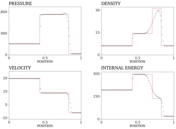
3.2 Second order HLLC solver with Van Albada slope limiter. The numerical (icon) and exact (line) solutions are shown for t= 0.2 and xdiaph = 0.5. 29 3.3 First order HLLC solver. The numerical (icon) and exact (line) solutions are shown fort= 0.15 andx0= 0.5. . . 30

3.4 Second order HLLC solver with Van Albada slope limiter. The numerical (icon) and exact (line) solutions are shown for t= 0.15 and xdiaph = 0.5. 31 3.5 First order HLLC solver. The numerical (icon) and exact (line) solutions are shown fort= 0.035 and xdiaph = 0.4. . . 32

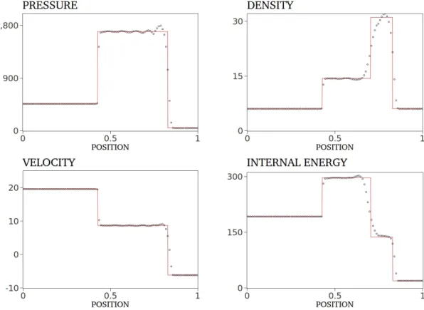
3.6 Second order HLLC solver with Van Albada slope limiter. The numerical (icon) and exact (line) solutions are shown for t= 0.035 and xdiaph = 0.4. 33 3.7 First order HLLC solver. The numerical (icon) and exact (line) solutions are shown fort= 0.012 and xdiaph = 0.8. . . 34

3.8 Second order HLLC solver with Van Albada slope limiter. The numerical (icon) and exact (line) solutions are shown for t= 0.012 and xdiaph = 0.8. 35 3.9 First and second order HLLC solver. The numerical (icon) and exact (line) solutions are shown fort= 2 and xdiaph = 0.5. . . 36

3.10 First (left) and second order (right) HLLC solver. The numerical (icon) and exact (line) solutions are shown fort= 2 and xdiaph = 0.5. . . 36

4.1 Fan rotor . . . 40

4.2 Measurement coordinates: radial position (RP), axial position (AP), circumferential position (CP) (after NASA TP2879 [6]) . . . 41

4.3 Streamlines (after NASA TP2879 [6]) . . . 42

4.4 Window numbering (after NASA TP2879 [6]) . . . 42

4.5 Streamline extraction in Paraview . . . 44

(19)

List of Figures

4.7 Blade-to-Blade mesh detail with repetition . . . 46

4.8 Mesh details . . . 47

4.9 3D mesh (fine) . . . 47

4.10 Boundary layer regions (after Bakker [7]) . . . 49

4.11 Mach number plot at 10% span from shroud near peak efficiency . . . . 53

4.12 Plot of ₋5.4% chord at 10% span . . . 54

4.13 Plot of 30% chord at 10% span . . . 54

4.16 Plot of 20% pitch at 10% span . . . 56

4.20 Plot of ₋10% chord at 30% span . . . 59

4.28 Plot of ₋10% chord at 70% span . . . 64

(20)

List of Figures

4.36 Relative total pressure at 10% span . . . 71

4.37 10% Span BIAS . . . 74

4.38 10% Span CI . . . 74

4.39 10% Span RMSE . . . 75

4.40 30% Span BIAS . . . 75

4.41 30% Span CI . . . 76

4.42 30% Span RMSE . . . 76

4.43 70% Span BIAS . . . 77

4.44 70% Span CI . . . 77

4.45 70% Span RMSE . . . 78

4.46 Tip gap vortex shedding . . . 80

4.47 Trailing edge vortex shedding . . . 81

5.1 Complete stage: orange - rotor blades; blue - stator blades; green - hub 86 5.2 Stage layout: blue - mixing plane . . . 87

5.3 Stage layout: blue - mixing plane grid . . . 89

(21)

LIST OF TABLES

2.1 Value ofW_i₊1

2 (0) required to evaluate the inter-cell flux (after Toro [5]) 16

4.1 Mesh cell number . . . 46

4.2 Boundary conditions . . . 49

4.3 Overall aerodynamic performance (numerical) . . . 69

4.4 Relative error . . . 69

4.5 Convergence time . . . 82

5.1 Rotor-stator mesh number . . . 89

(22)

(23)

LIST OF SYMBOLS

Abbreviations

3D Three dimensional

Π Total pressure ratio

ALE Arbitrary Lagrangian-Eulerian

AP Axial Position

ARS Approximate Riemann Solver

B2B Blade to Blade

BV Blade Vortices

CFD Computational Fluid Dynamics CHT Conjugate Heat Transfer

CI Concordance Index

CP Circumferential Position

CV Coriolis Vortices

DNS Direct Numerical Simulation

DS Domain Scaling

FNMB Full Non Matching Boundary FSI Fluid-Structure Interaction GGI General Grid Interface GUI Graphic User Interface

(24)

List of Symbols

IP Intermediate Pressure IRS Implicit Residual Smoothing

LA Laser Anemometer

LE Leading Edge

LES Large Eddy Simulation LMSC Lp Metric Space Condition

LP Low Pressure

LTS Local Time Stepping

MP Mixing Plane

MUSCL Monotone Upstream-Centered Schemes for Conservative Laws NACA National Advisory Committee for Aeronautics

NASA National Aeronautics and Space Administration NHM Nonlinear Harmonic Method

PS Pressure Side

PV Passage Vortices

r_×θ-M Radius_×Theta-Meridional

R67 Rotor 67

RMSE Root Mean Square Error

RP Radial Position

SS Suction Side

SST Shear Stress Transport

TE Trailing Edge

TVD Total Variation Diminishing

WNBEG Starting Window Number for Laser Anemometer Survey

Greek Symbols

δij Kronecker delta

-η Efficiency

-γ Specific heat ratio

(25)

List of Symbols

ν Kinematic viscosity m2s−1

Ω Vorticity s−1

ω Specific dissipation rate s−1

φ Adimentional velocity

-Π Pressure ratio

-ψ Adimentional work

-ρ Density kg m−3

σ Total shear stress tensor; Effective turbulent quantity kg m−1−2s

τ Shear stress kg m−1−2_s

τt Pseudo time-step s

υ Volume m3

ε Turbulent dissipation m2s−3

ϕ Arbitrary quantity

-Subcripts

0 Total quantities

1 Rotor inlet (note the ambiguity with Runge-Kutta coefficients) 2 Rotor outlet (note the ambiguity with Runge-Kutta coefficients)

a Adiabatic

c Convective terms

d Dissipative terms

i Cell index (note the ambiguity with the matrix index) l, L Left

r, R Right

s Static quantities

t Temporal term

∗ Star Region

blade, rot Blade diaph Diaphragm

(26)

List of Symbols

Lam Laminar

max Maximum

min Minimum

r,θ,z Cylindrical directions

sw stream-wise

-T urb Turbulent

x,y,z Cartesian directions

Supercripts

T _Transpose

n+1 _{Next time step}

n _{Current time step}

Mathematical Symbols

∆ Difference operator

-∂

∂ Partial derivative operator

-∇ Gradient operator

-∇· Divergence operator

-∇·∇ Laplacian operator

-ℜb Blade-to-Blade radius m

ℜn Meridional radius m

sup Supremum operator

-F Flux tensor

-Fhllc Godunov flux

-R Residual vector

-U Conservative state vector

-W Primitive variables

-˜

A Mass-averaged of an arbitrary quantity

-~

U Absolute velocity vector m s−1

~

Urel Relative velocity vector m s−1

(27)

List of Symbols

A′′ Arbitrary quantity fluctuation

-c, a Sound velocity m s−1

Ccf l Courant-Friedrich-Lewy number

-Cp Specific heat (constant pressure) kJ kg−1K−1

E Energy kJ

F Decomposed flux tensor in an arbitrary referential

-h Enthalpy kJ kg−1

K, k Turbulent kinetic energy m2s−2

M a Mach number

-O Order

-P,p Pressure kg m−2

P r Prandt number

-Re Reynolds number

-S Wave speed m s−1

Sij Mean strain tensor s−1

T Temperature K

t Time s

u, v, w Velocity components in a Cartesian referential m s−1

V, U Magnitude of (absolute) velocity m s−1

Vθ Tangential velocity m s−1

W Magnitude of relative velocity m s−1

x, y, z Cartesian coordinates m

Y+ Dimensionless distance to wall

-R Specific gas constant kJ kg−1_K−1

r,θ,z Cylindrical coordinates

(28)

(29)

CHAPTER

1

INTRODUCTION

Turbomachinery plays an important role in the industry, in the world’s energy supply and mobility. From an engineering perspective, its applications can be divided into their governing physics: compressible and incompressible flows. This work only concerns the former.

Turbomachines ruled by compressible flows are designed to create a great pressure differential. The most sounding example is the gas turbine cycle used in airplanes, automobiles and even boats: air flows through compressors, combustors and turbines. The latter extracts some if not all energy, depending on the applications, i.e. a fighter doesn’t need to pass much energy to a shaft while in a Thermoelectric, that is the main purpose.

Although there are considerably distinct applications, the flow structures are similar between all and it becomes important to understand how they work in detail. Com-putational Fluid Dynamics (CFD) and the advance in computing performance in the last decades allowed complex and large simulations to be made in reasonable time, thus much of the pre-project budget is reduced. Furthermore, it has proved to be a pow-erful research tool when examining complex physics and multi-phenomena interaction, namely on turbomachinery.

(30)

compu-Introduction

tational methods can be used with safety. The motivation of this thesis is to add reliability to the steady density based solver implemented by Borm et. al. [8] in the OpenFOAM libraries: the transonicMRFDyMFoam. Moreover, the code used in this thesis is open-source which clearly is an advantage compared to commercial codes.

The main objective of this thesis is to solve a three dimensional (3D) flow of an aircraft fan component, the NASA Rotor 67, and compare it with experimental data. A fan is a low pressure (LP) compressor which is part of a turbofan’s compressor set (Figure 1.1). It is responsible for generating about 80% of the engine’s thrust in common commercial airplanes. Statistical tools and plots will show how well data matches.

Figure 1.1: Turbofan’s compressor set: LP, intermediate pressure (IP), high pressure (HP) compressors (Courtesy Rolls Royce [1])

This thesis will also present some simple tests, called Riemann problems, that show how accurate the hyperbolic system in the Navier-Stokes equations is solved. By last, a numerical feature specially designed to turbomachinery is tested: the mixing plane. It allows steady multi-row problems to be solved which gives strength to OpenFOAM as a reliable alternative to commercial software.

(31)

phenom-Compressible flow

ena that are useful when dealing with turbomachinery. Chapter 2 will describe the numerical methods that build the OpenFOAM’s transonic density-based solver while Chapter 3 presents the Riemann problems. Chapter 4 is the highlight of the thesis and will present the NASA Rotor 67. Chapter 5 presents the multi-row simulation and Chapter 6 is reserved for final appreciations and conclusions.

1.1 Compressible flow

Compressible flows are considered when fluid velocity is above Mach (M a) 0.3, be-coming comparable with sound velocity, M a = 1. In air, sound velocity is a func-tion of state, i.e. funcfunc-tion of static temperature (Ts). Flows in the transonic region, 0.8< M a <1.2 are a characteristic of turbomachinery thus they are the focus of this thesis. When in presence of such flows, some phenomena may happen: they are shock waves, choked flows and surge flows.

Shock waves [9] start to exhibit when flow enters the transonic region and they are characterized by a thermodynamic state discontinuity, usually velocity decreases with an increase ofPs andTs. They indeed provoke a compression, which is the objective of a compressor, but are mainly a source of losses and noise. Shock waves in wall bounded flows have and additional complexity because there exists an increased interaction with the boundary layer (Figure 1.2).

Figure 1.2: Normal shock in a wall bounded flow: interaction between shock and boundary layer can be seen (after Korpela [2])

(32)

Introduction

It is demonstrated for isentropic flows [10] that this critical section imposes a maximum mass flow. This phenomena obviously must be taken in mind when projecting a duct, or more precisely a turbo-machine, because depending on their geometry , mass flow will always be limited.

Surge flows exhibit when flow incidence in compressor blades starts to be misaligned with their metallic angles: separation produces losses and instability. This phenomena is closely related to stall: it usually happens with low mass flow and airflow can simply stop, entering a surge cycle (Figure 1.3).

Another compressible flow effect is that air compressibility can no longer be ne-glected meaning that density (ρ) of air will change. For further details see White [10] or Anderson [9].

Figure 1.3: Surge cycle: strong separation makes airflow stop (stall) and high pres-sure air downstream rushes back through compressor. When back-flow stops, airflow is reestablished and the cycle repeats itself (Courtesy of Thy-Engineering; Private com-munication)

1.2 Turbomachinery

(33)

Turbomachinery

is what you feel if you were moving with the flow. Total quantities is what you would feel if you could grab the flow and adiabatically take the velocity to zero. In other words, total quantities take into account kinetic energy and it is usual to define the following [2]: total enthalpy (Eq. 1.1), total pressure (Eq. 1.2) and total temperature (Eq. 1.3).

h0 =h+

V2

2 (1.1)

withh=CpTs being the static enthalpy,Cp the specific heat at constant pressure and V the magnitude of absolute velocity.

P0=Ps×(1 + γ₋1

2 M a

2₎_γ₋γ₁ _(1.2)

T0 =Ts×(1 + γ₋1

2 M a

2₎ _(1.3)

with M a = V c, c=

p

γRTs is the speed of sound,γ the specific heat ratio and R the specific gas constant.

It follows that overall aerodynamic parameters [6] can be defined and will be used in the next chapters. They are adiabatic efficiency (Eq. 1.4) and total pressure ratio (Eq. 1.5),

ηa=

P02

P01 (γ−1)

γ

−1 T02

T01 −1

(1.4)

Π = P02 P01

, (1.5)

where subscripts1 and 2 denote inlet and outlet of the rotor, respectively.

1.2.1 Compressor flow

Compressor flow is characterized by a deceleration of relative velocities. It can be seen in Figure 1.4 the Euler velocity triangles of a rotor and a stator. The work done by the blades [2] is related to the change in tangential velocity (Vθ), according to Eq. 1.6.

(34)

Introduction

withUbladebeing the blade velocity.

Figure 1.4: Euler triangle velocities in a compressor stage; exceptional notation for blade velocityU (after Korpela [2])

Compressors are designed for the flow to achieve a pressure ratio at a specific mass flow. It is called the design point and it is thought to be the point where the compressor will work more often. Usually, there will be more points where the compressor needs to work and it will be limited by the choked mass flow and surge or stall conditions. Therefore, every compressor has a map closely related to Figure 1.5: ψ and φdenote dimensionless work and velocity, respectively. It can be advanced that a map for NASA Rotor 67 will be made in Chapter 4.

(35)

Turbomachinery

It is important to remark some phenomena in compressor flows that will gain bigger relevance in next sections. There is a clearance between the blade and the casing called Tip-Gap: flow that goes through that gap is calledtip leakage. Figure 1.6 shows a flow structure provoked by the tip-gap: a tip vortex. It is created because the suction and pressure side don’t have a surface to separate them in the gap and so they struggle to get mixed. In Chapter 4 this situation will be simulated and illustrated.

Figure 1.6: Tip-gap flow structure (after Tang [3])

Under certain conditions there is also separation induced by passage shock/bound-ary layer interaction which was seen in Figure 1.2. By last, secondshock/bound-ary flows may appear too and will be described next.

1.2.2 Secondary flows

Secondary flows are seen as the difference between the 3Dinviscid solution and the real viscous flow happening in turbomachinery flows. Van den Braembussche [4] pointed out recently that this flows redistribute low energy fluid, due to blockage, through the stream-wise vorticity influencing the inviscid core velocity and pressure.

(36)

Introduction

The first two right hand side terms of Eq. 1.7 express the generation of vorticity due to flow turning in meridional and blade-to-blade (B2B) planes, respectively. The last term represents generation of vorticity due to Coriolis forces. Thus, second and third term generate passage vortices (PV), first term generates vortices along blade vortices (BV) and again third term also generates Coriolis vortices (CV). _ℜn and ℜb stand for curvature radius in meridional and B2B plane, respectively. Ωs is the stream-wise vorticity and s denotes streamline. Figure 1.7 presents a scheme of these vortices. Further details in [4] [11].

(a) PV vortices

(b) BV vortices

(c) CV vortices

(37)

CHAPTER

2

NUMERICAL METHODS

This chapter will introduce the numerical methods used by Borm et. al. [8] to im-plement the transonic density-based libraries [12] in OpenFOAM. These libraries have mainly two solvers, the steadytransonicMRFDyMFoamand the unsteady transonicUn-steadyMRFDyMFoam. It is also available anarbitrary Lagrangian–Eulerian(ALE) [13] method for moving meshes like Fluid-Structure Interaction (FSI) or rotating compo-nents and a Conjugate Heat Transfer (CHT) formulation.

In the main solvers, primitive variables [ρ, U, p]T are reconstructed by a Monotone Upstream-Centered Schemes for Conservative Laws (MUSCL) [14]. Then, they are used as an input to an upwind approximate Riemann solver (ARS) which will return the inviscid numerical fluxes. These were first used in a Godunov scheme [5] to solve the Euler equations.

(38)

Numerical Methods

2.1 Navier-Stokes equations

The complete form of the N-S presented in the differential form [16] is read

∂U

∂t +∇·Fc(U) =∇·Fd(U,∇U) (2.1) where Uis a conservative state vector

U=         ρ ρu ρv ρw ρE         (2.2)

Fc = (Fcx, Fcy, Fcz) is the convective flux tensor

F_cx =

        ρu ρu2+p

ρuv ρuw (ρE+p)u

       

, F_cy =

        ρv ρvu ρv2+p

ρvw (ρE+p)v

       

, F_cz =

        ρw ρwu ρwv ρw2+p (ρE+p)w

        (2.3)

Fd= (Fdx, Fdy, Fdz) is the dissipative flux tensor

F_dx =

        0 τxx τxy τxz

uτxx+vτxy+wτxz+qx

       

, F_dy =

        0 τyx τyy τyz

uτyx+vτyy+wτyz+qy

        ,

F_dz =

        0 τzx τzy τzz

uτzx+vτzy+wτzz+qz

        (2.4)

and τij the dissipative stress tensor

τij =



 

τxx τxy τxz τyx τyy τyz τzx τzy τzz





, (2.5)

(39)

RANS equations in a rotating referential

If viscosity and thermal conduction is neglected one arrives to the Euler equations, which are solved first by Godunov for compressible flows [5].

When dealing with problems that admit discontinuities (i.e. shocks) it becomes necessary to solve the N-S equations in a conservative form. Non-conservative numerical schemes will fail in providing the right shock speed if we are in presence of a Riemann problem [5]. As Zanoti and Manca [17] remember, Hou & Le Floch [18] proved that non-conservative schemes do not converge if a shock wave is part of the solution while Lax & Wendroff [19] showed that conservative schemes, if convergent, they converge to the weak solution of the problem.

2.2 RANS equations in a rotating referential

In order to solve turbulence in a practical way, the transonic density-based libraries are implemented under the N-S equations with mean flow quantities: the so called called Reynolds-Average Navier-Stokes (RANS) equations. In fact, for compressible flows, there is a variation of RANS equations called Favre-average Navier-Stokes. If the first uses a time average of the quantities, its variant uses a mass-average because density indeed changes in compressible flows. Hereinafter this work will use the Favre equations but the reference to the Reynolds-Average Navier-Stokes will remain the same.

Flow quantities of RANS are defined by

A= ˜A+A′′ (2.6)

where the double prime is the fluctuation and the tilde is the mass-average quantity and has the form

˜ A= ρA

¯

ρ (2.7)

with

ρA_≡ 1 ∆t

Z t0+∆t

t0

ρAdt. (2.8)

(40)

Numerical Methods

Reynolds Stress)

(τij)T urb=−ρu′′iu

′′

j (2.9)

(qj)T urb=−CpT′′ρu′′_j. (2.10)

The so called closure of the RANS equations is made by expressing the Reynolds stress (Eq. 2.9) with the mean quantities. For most well known turbulence models (i.e. Spalart Allmaras [21], k₋ω [22], k₋ω SST [23]) this is done with a linear relation between Reynolds stress and the mean strain tensorSij

Sij = 1 2

h_∂_U˜_i

∂xj

+∂U˜j ∂xi

i

(2.11)

that is read

(τij)T urb=−2µT urb

Sij ₋1 3

∂U˜k ∂xk

δij+2

3ρ˜Kδij˜ . (2.12)

Eq. 2.12 is analogous to the linear constitutive equation for Newtonian flows

(τij)Lam=−2µLam

Sij− 1 3

∂U˜k ∂xk

δij

, (2.13)

being (τij)Lam the laminar stress tensor: this analogy is called Boussinesq hypothesis [24]. Note the last term in Eq. 2.12 is added to correct the trace of Reynolds stress [25]. Eq. 2.9 and 2.12 are very popular and are worth some comments. They have been the base for development of the most used turbulence models in industry but fail in physical meaning. Even for the simplest flow, concepts such as fluctuating velocities don’t seem to have solid experimental support neither have an explicit derivation from equations. Schmitt [24] reviewed in the detail the work of Boussinesq, pioneer of mean quantities in NS equations, and pointed its major weakness: a bad extrapolation of molecule kinetic energy theory to turbulent flows is made concerning the mean free path of molecules.

(41)

Hyperbolic system solution

state assumptions are valid. G¨on¸c [26] and Borm [8] write them in vectorial form, where quantities are already in their mean value

∂ρ

∂t +∇·(ρ ~Urel) = 0 ∂ρ ~U

∂t +∇·(ρ ~Urel⊗U~) +∇p = −ρ(w~×U~) +∇·σ ∂ρE

∂t +∇·((ρE+p)U~rel+p ~Urot) = ∇·(σ·U~)− ∇·~q+∇·(µ+β

∗_µ

T)∇K (2.14)

σ= (µLam+µT urb)

∇U~ + (_∇U~)T ₋2

3(∇·U~)δij

−2₃ρKδij. (2.15)

Note that Eq. 2.15 is the total shear stress tensor and it is the sum of Eq. 2.12 and 2.13. It is usually called effective turbulent quantity [16].

2.3 Hyperbolic system solution

The transonic density-based solvers implemented in OpenFOAM by Borm et. al. [8] use an ARS to calculate the inter-cell’s flux based on characteristic’s speed. Then, a Godunov scheme solves the hyperbolic system.

2.3.1 Godunov scheme

The Godunov scheme can be written in the conservative form [5]

Un_i+1=Un_i + ∆t

∆x Fi−1/2−Fi+1_/2

. (2.16)

To understand how the Godunov scheme is assembled, one must consider the fol-lowing conservative form of the 1D Euler equations

Ut+F(U)x= 0, (2.17)

with the conservative state vector and the flux

U=    ρ ρu ρE  

 F=



 

ρu ρu2+p (ρE+p)u





(42)

Numerical Methods

One can divide the spacial domain inN computing cellsIi=xi−1_/2, xi+1_/2

of length ∆x=xi+1_/2−xi−1_/2 with a “height” of ∆t=

tn₋tn+1 (Figure 2.1). Integrating Eq. 2.17 on cell Ii, first in space and then in time, it results the following

Z x_i₊₁_/₂ x_i₋1/2

U x, tn+1dx=

Z x_i₊₁_/₂ x_i₋1/2

U(x, tn)dx+

Z t+1

t

F U xi−1/2, t

−

Z t+1

t

F U xi+1/2, t

.

(2.19)

Figure 2.1: Computational mesh (after Toro [5])

At this point two concepts are introduced. Eq. 2.20 makes some information being lost and the scheme to be first order. This is called the piecewise constant data [5] and it is the first concept. It is convenient to note that in order to make this averaging, waves can’t interact (Figure 2.2). The second (Eq. 2.21) is the Godunov flux or inter-cell numerical flux. Rewriting Eq. 2.20 and Eq. 2.21 into Eq. 2.19 one arrives to the Godunov scheme.

Un_i = 1 ∆x

Z x_i₊₁_/₂ x_i₋1/2

U(x, tn)dx (2.20)

F_i_±1_/2 =F

U x_i_±1_/2, t

(43)

Figure 2.2: Godunov averaging of local solutions to the Riemann problem within cell Ii at fixed time ∆t (after Toro [5])

Other note about this scheme is that in order to prevent the interaction of waves described above, the time step ∆t must satisfy the following condition,

∆t_≤ Ccf l∆x Sn

max

(2.22)

withS_maxn being the fastest wave speed in the domain at timetn. This is the so called Courant-Friedrich-Lewy (CFL) condition [27] and Ccf l is the CFL number . For the 3D Euler system, results follow similarly.

2.3.2 Solution of the Riemann problem in the Euler equations

Considering the following initial valued problem with discontinuous data, the Riemann problem [5]

Hyperbolic system : Ut+F(U)x = 0, Initial condition : U(x,0) =U(0)(x),

Boundary condition : U(0, t) =Ul(t), U(L, t) =Ur(t),

(2.23)

in a domain xl < x < xr using the explicit conservative formula of Eq. 2.16. The Godunov flux at interfacex_i₊1_/2 is defined by

F_i₊1 2 =F

U_i₊1

2 (0)

, (2.24)

beingU_i₊1

2 (0) the exact similarity solutionUi+12(

(44)

Numerical Methods

2.1 shows all the possible state solutions W_i₊1

2 (0). Note that they are computed as

primitive variables and the star region is the space between the fastest and slowest speed waves (Figures 2.3 and 2.4).

Sub-case Case (a) positive speedu_∗ Case (b) negative speed u_∗

1 WL WR

2 W_∗L W∗R

3 WL WR

4 W_∗L W∗R

5 WLf an WRf an

Table 2.1: Value of W_i₊1

2(0) required to evaluate the inter-cell flux (after Toro [5])

Figure 2.3: Wave pattern possibilities; a) positive particle velocity in star region b) negative particle velocity in star region; Thick, dashed and multi lines represent shock, contact and rarefaction waves (after Toro [5])

For example, considering the situation in whichu_∗is positive, to calculateW_i₊1 2 (0)

one must identify the character of the left wave. If it is a shock, one calculates the state

W_∗L between the contact and shock wave through shock relations [5]. Than the speed SL of the left shock is computed. IfSL_≥0 it is said supersonic and

W_i₊1

(45)

If SL≤0 it is said subsonic and

W_i₊1

2(0) =W∗L. (2.26)

It follows that the inter-cell flux is calculated by Eq. 2.27 and the remaining possibilities presented in Figure 2.3 are solved in a analogous way.

F_i₊1 2 =F

W_i₊1

2 (0)

(2.27)

This method is the exact1 solution of the Riemann problem applied to the Euler equations but it is not efficient due to large number of iterations. Next section will present an approximate Riemann solver called Harten Lax Van Leer Contact (HLLC) which is more practical and it is used in all simulations.

2.3.3 The HLLC approximate Riemann solver

Harten, Lax and Van Leer (HLL) [28] introduced the HLL approximate Riemann solver which consisted in defining a new wave structure. Because they considered just two waves [5], the solver becomes unacceptable when solving the Euler equations: the contact wave is missing and has an important physical meaning.

Toro, Spruce and Spears [29] introduced the HLLC approximate Riemann solver that takes the HLL and recovers the contact wave. The star region is composed by two states and the structure of the solution is presented in Figure 2.4.

Figure 2.4: Structure of the HLLC approximate solution (after Toro [5])

Then, the HLLC solver is given by

(46)

Numerical Methods

˜

U(x, t) =

              

UL if x

t ≤SL

U_∗L if SL≤ x

t ≤S

∗

U_∗R if S∗≤ x

t ≤SR

UR if x

t ≥SR

(2.28)

By applying the Rankine-Hugoniot conditions [30] and relating the states in the star region [5], the Godunov flux to be applied into the Godunov scheme can be written as

Fhllc_i₊1 2 =           

FL if

x t ≤SL

F_∗L=FL+SL(U∗L−UL) if SL≤x/t≤S∗

F_∗R=FR+SL(U∗R−UR) if S∗ ≤x/t≤SR

FR if

x t ≥SR

(2.29)

It only remains to calculate the wave speeds which can be done directly from data

SL=uL−aL, SR=uR+aR (2.30)

and

SL=min{uL−aL, uR−aR}, SR=max{uL+aL, uR+aR}. (2.31)

whereu denotes the particle speed and athe sound speed. For different approaches in calculating wave speeds or more details about the Riemann problem, see Toro [5].

2.4 Turbulence modeling

It is widely accepted that the 3D N-S are the correct representation of turbulent flow [31]. Every length scales are modeled in a RANS approach whether in Large Eddy Simulation (LES) only the smallest scales [32] are modeled. In Direct Numerical Simulations (DNS) every scale is calculated which leads to the need of massive com-putational resources. Landmann [16] rescues Kolmogorov and its micro-scale theory, pointing out that one needs O(Re3/4_{) to resolve all turbulent length scales per space}

dimension. Due to the fact that turbulence is a three dimensional phenomena, one would need O(Re9/4_{) grid cells.}

(47)

Turbulence modeling

viscosityµT. Borm [8] points out there might be some conflict in rotor-stator problems when using a turbulence model that use vorticity terms because velocity jumps in the interface. The Shear stress transport model was used and doesn’t have this problem: it is described below.

2.4.1 Shear stress transport (SST)

The SST model, introduced by Menter [23], is a two equation model that takes the approach of the k₋ω [22] at the inner region of the boundary layer, using the k₋εin the outer region and free-stream. It modifies the definition of eddy viscosity by taking into account the transport of turbulent shear stress. This modification proved to be very important for accuracy in adverse pressure gradients [33] which is a requisite in aerodynamic turbulence models [34]. The k₋ω formulation makes it robust and a good choice for the logarithmic and viscous sublayer regions. For the outer region and free-stream, k₋ω predictions are very sensible to the free-stream specific dissipation rate ω, therefore SST switches to k₋ε model which hasn’t this behavior. In SST transport equations one can read the (1) Lagrangian derivative, (2) production term, (3) destruction term and (4) the dissipation term

k: Dρk Dt

| {z } 1

=τij ∂ui ∂uj

| {z } 2

−β∗_ρωk

| {z } 3

+ ∂ ∂xj

h

(µLam+σkµT urb) ∂k ∂xj

i

| {z }

4

(2.32)

ω : Dρω Dt

| {z } 1 = γ νT τij ∂ui ∂uj

| {z }

2

−β∗ρω2

| {z } 3

+

∂ ∂xj

h

(µLam+σωµT urb) ∂k ∂xj

i

+ 2ρ(1₋F1)σω2

1 ω ∂k ∂xj ∂ω ωxj

| {z }

4

(2.33)

where constants2 Ckω,Ckε correspond to k−ω model,k−ε, respectively

Ckω       

σk1 = 0.85 σω1= 0.5 β1 = 0.0750

β∗ = 0.09 k= 0.41 γ1 =

β1

β∗ −σω1k

2

/√β∗

(48)

Numerical Methods Ckε       

σk2= 1 σω2= 0.856 β2 = 0.0828

β∗ = 0.09 k= 0.41 γ2 =

β2

β∗ −σω2k

2

/√β∗

.

The constantsCkωSST will result of a combination betweenCkω andCkεthat reads

CkωSST =F1Ckω+ (1−F1)Ckε (2.34)

and the model closes with the following relations

F1 =tanh    (" max √ k β∗_ωd,

500ν d2_ω

!

, 4σω2k CDkωd2

#)4





, (2.35a)

F2 =tanh   " max 2 √ k β∗_ωd,

500ν d2_ω

!#2

, (2.35b)

CDkω =max

2ρσω2

1 ω ∂k ∂xi ∂ω ∂xi

,10−10

, (2.35c)

νT urb =

a1k

max(a1ω,ΩF2)

, (2.35d)

beingνT urb the kinematic turbulent viscosity.

The derivation of Eq. 2.32 and 2.33 comes from a transformation of thek₋εmodel to a k₋ω formulation with the following relation

ω= ε

β∗_k. (2.36)

and then a combination of both k₋ε and k₋ω models with a function F1 that acts

like a switch in the inner and outer regions of the boundary layer. Full details are given by Davidson [35].

There are variations of the model with different approaches [36] [37].

2.5 Space discretization

(49)

Space discretization

The interpolation formulae of the inviscid terms is done with Van Leer’s MUSCL [14] which defines them as second-order accurate in space.

Taking the Godunov integral average for a specific quantityϕn_i in cellIi = [xi−12, xi+12],

the piece-wise linear reconstruction of MUSCL is given by

ϕi(x) =ϕn_i +(x−xi)

∆x ∆ϕ, x∈[0,∆x] (2.37)

where ∆ϕ

∆x is a chosen slope of ϕi(x) in cell Ii. Figure 2.5 shows the average and its linear reconstruction.

Figure 2.5: Piece-wise linear reconstruction for three successive cells (after Toro [5])

It is also of great importance the extreme points ofϕi(x), they will define the right ϕi+1_/2 and leftϕi−1_/2 states introduced in Section 2.3.2 and are given by

ϕi−1_/2 =ϕni − 1

2∆ϕ, ϕi+1/2=ϕ n i +

1

2∆ϕ. (2.38)

The slope is read

∆ϕ= 1

2(1 +ω)∆ϕi−1/2+

1

2(1−ω)∆ϕi+1/2 (2.39)

with

∆ϕ_i₋1_/2 ≡ϕ

n

i −ϕni−1, ∆ϕi+1_/2 ≡ϕ

n

(50)

Numerical Methods

In all simulations the Venkatakrishnan [39] limiter is used. It is second order accu-rate ω= 0 and reduces the reconstructed gradient by the following factor

Ψ =                  1 ∆2 " ∆2

1,max+ǫ2

∆2+ 2∆22∆1,max ∆2

1,max+ 2∆22+ ∆1,max∆2+ǫ2 #

if ∆2>0

1 ∆2





∆2₁_,min+ǫ2∆2+ 2∆22∆1,min ∆2

1,min+ 2∆22+ ∆1,min∆2+ǫ2 

 if ∆2<0

1 if ∆2= 0

(2.41)

where

∆1,max=φmax−φi∆1,min=φmin−φi. (2.42) In Eq. 2.42,φmaxandφminare the maximum and minimum values of all neighbor nodes and the owner itself. The parameter ǫ2 is meant to control the amount of limiting and it was found that it should be proportional to a local scale length, i.e.

ǫ2 = (K∆h)3 (2.43)

It was found [39] that settingK = 5 provided the best convergence properties with the best shock resolution thus this value is used in all simulations.

Other limiters are implemented such as Barth-Jespersen [40] and Minmod [41]. The upgrade of MUSCL with limiter schemes is also called Total Variation Diminishing (TVD) schemes.

The viscid terms are build with central difference discretization which is second order. Therefore, this solver is second order in space although lower order can be used.

2.6 Time discretization

2.6.1 Steady solver

For each control volume, Eq. 2.1 can be written in a semi discrete form

∂υU

∂t =−R(U) (2.44)

(51)

Time discretization

time, one can reach a steady state R(U) = 0 or an unsteady solution. Although both solutions are available in the density-based libraries, just the former will be presented in detail.

It is important to note that time accuracy in steady cases is irrelevant. The accuracy of the solution only depends on spacial discretization making the advantage of method of lines clearer. From the other side, in unsteady flows, the aim is to get the highest temporal accuracy possible not forgetting stability and computational costs issues.

Runge-Kutta [42] time stepping is available and will used in all simulations. It is given by

U0=Un

U1=U0₋α1

∆t ∆xR(U

0₎

U2=U0₋α2

∆t ∆xR(U

1₎

U3=U0₋α3

∆t ∆xR(U

2₎

U4=U0₋α4

∆t ∆xR(U

3₎

Un+1 =U4

(2.45)

and the following coefficients were used in all simulations α1 = 0.11

α2 = 0.2766

α3 = 0.5

α4 = 1.0

. (2.46)

By reducing the residual of equation 2.44 towards machine zero, a steady state will be reached. Convergence measures will be introduced in Section 2.8.

2.6.2 Unsteady solver

The unsteady solver will only be used in Chapter 3 to solve the Riemann problems. The approach to calculate an unsteady problem used in this solver calleddual time-stepping (DTS) and it a is common practice. Explicit Runge-Kutta and convergence acceleration techniques are not time accurate and so, Jameson [43] introduces a pseudo-timeτ solver that will reformulate Eq. 2.44 the following way

∂υU

∂τt

= ∂υU

∂t +R(U) =R

(52)

Numerical Methods

R∗(U) is a new residual and the physical time derivative ∂

∂t is approximated by a second order accurate three-point backward difference [44]. Hence,

∂υU

∂τt = 3υ

n+1_Un+1₋_4υn_Un₊_υn−1_Un−1

2∆t +R(U

n+1_{) =}_R∗₍_Un+1_), _(2.48)

with the steady state techniques mentioned above being used to reduce the residual

R∗(U). When the pseudo-time solver converges ∂ΩU ∂τt ≈

0, the physical time step advances.

2.7 Accelerating convergence techniques

Here is described the only accelerating convergence technique implemented in the density-based libraries: the Local Time Stepping (LTS).

The LTS consists in using the maximum allowable time step taking the dissipative and convective contributions. Hence, according to Blazek [44] they can be given by

∆td=max

4 3ρ, γ ρ µLam P rLam

+ µT urb P rT urb

(∆x)2

υ , ∆tc= (|U|+c) ∆x (2.49) and Andrea [45] proposes the following final time step

∆t=Ccf l

∆td∆tc ∆td+ ∆tc

. (2.50)

Other accelerating convergence techniques are Implicit residual smoothing (IRS) and Multigrid. IRS is a technique to diminish the dependence of time steps from CFL number and consequently raise the maximum time step. Applying IRS in the explicit multistage scheme mentioned in section 2.6 was introduced by Jameson [46] and consists in replacing the residual for an average of neighbor’s residuals.

(53)

Convergence in metric spaces L2 and L∞

2.8 Convergence in metric spaces

L

2

and

L

∞

Metric spaces are a useful tool to see how much converged a solution is. In fact, it is the metric on Rthat defines the concept convergence of a sequence [50].

A metric space is a setXof elements whose nature is left unspecified, with a distance function d defined on it [50]. It is convenient to note that the pair (X, d) is a metric space if dsatisfies some conditions.

TheL∞(X, d) metric space is the set X of all bounded sequences with the metric

d(x, y) = sup j∈N|

ξj₋ηj_| (2.51)

whereξj andηjare sequences of the set. Here it is enough to say, without the proof [50], thatL∞ is a complete metric space (Banarch space). ACauchy sequence is a sequence

{xn_}∞_n₌₁ such that

∀ǫ >0 _∃Nǫ _⇒d(xn, xm)< ǫ _∀n, m < Nǫ. (2.52)

Again, without the proof, it follows that all Cauchy sequences converge in complete spaces.

The Lp metric space is a set of sequences x = (ξj) = (ξ1, ξ2,· · ·) such that |ξ1|p+ |ξ2|p+· · ·3 converges. The metric reads

d(x, y) =





∞

X

j=1

|ξj−ηi|p



 1/p

. (2.53)

Setting p= 2 one arrives to the well knownHilbert sequence space L2 [51].

Applying these concepts to CFD and more precisely to residuals, one can make the following analogy. Every cell’s residual can be seen as a sequence and the whole mesh is the set of sequences: it is true that at each step they have a value. If a steady state is to be reached, LMSC is true and we can measure thesteadiness with Eq. 2.53. Moreover, LMSC is a Cauchy sequence thus we are sure it will converge in L∞_.

In a practical way, by plotting the metrics of bothL2 and L∞, some results follow naturally and can be mathematically proven:

(54)

Numerical Methods

if the problem is steady, the residual can definitely be interpreted as a sequence

inL2 and its metric will converge tod(x, y) = 0;

the metricd(x, y) in L2 gives a qualitative measure ofsteadiness;

if the residual can be interpreted as a sequence inL2, LMSC will converge inL∞;

the solution is said to be converged if and only if both the L∞ and L2 metrics reduces its order to an arbitrarily value ǫ;

convergence inL2 implies convergence inL∞_{but the inverse need not to be true.}

2.9 Comments on OpenFOAM

OpenFOAM is an open-source software which uses an unstructured mesh connection by nature, thus all numerical schemes must be implemented accordingly. Being unstruc-tured makes it very versatile when dealing with cell shapes [52] which allows higher mesh quality in complex geometries and easier local refinement.

Its creator Weller and chief architect Jasak planed it with an object oriented pro-gramming technique [53] that allows the user to extend functionalities as he pleases in a consistent manner, thus being highly customizable. OpenFOAM is available under a GNU General Public License and it is free.

Parallel computation is handled via a domain decomposition method [54] and is often available in all solvers. The steady solver used in this thesis supports paralleliza-tion except when using the mixing plane4 and when performing unsteady simulations. Finally, both of these solvers run with OpenFOAM’s version 1.6-ext.

(55)

CHAPTER

3

RIEMANN PROBLEM VALIDATION

This chapter checks the performance of the ARS used in this thesis and, consequently, the ability of Borm’s code implementation to catch shock, rarefaction and contact waves. Moreover, second order extensions will be compared to first order and the performance of the limiters will be accessed.

Recalling Section 2.3, the Riemann problem in the Euler equations is a discontinu-ous initial valued problem with a leftUL= [ρ, U, p]T and right stateUR whose solution is approximated with the propagation of three waves through the medium. This ap-proximation is done by an ARS and the one being used is the HLLC. Physically, this situation is illustrated as two states separated by a diaphragm: att= 0 the diaphragm is broken. Solutions are naturally evaluated at t >0.

The computational domain used for all the following tests is a one dimensional mesh defined such that x_∈[0,1]. It is discretized in 100 cells and the notation xdiaph denotes the position of the diaphragm. All tests are compared with the exact solution of Riemann-problem provided by Toro and all data is non-dimensional.

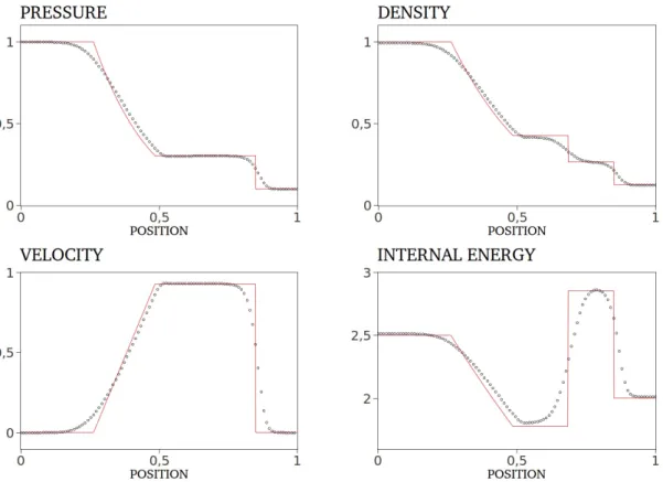
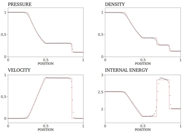
3.1 Sod’s shock tube

(56)

Riemann problem validation

is composed byUL= [1,0,1]T , UR= [0.125,0,0.1]T.

(57)

Sod’s shock tube

Figure 3.2: Second order HLLC solver with Van Albada slope limiter. The numerical (icon) and exact (line) solutions are shown fort= 0.2 andxdiaph= 0.5.

(58)

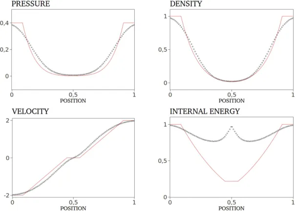
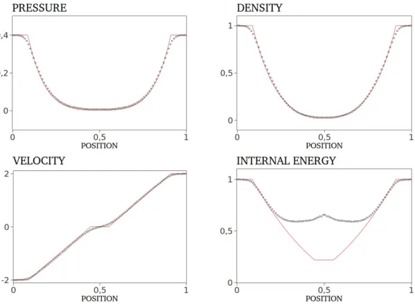
3.2 123 problem

This Riemann problem consists of two rarefaction waves and a trivial stationary contact discontinuity. The region between the two waves is characterized by very low pressure, close to vacuum, and this test is usually done to evaluate the solver’s ability to deal with low density flows. The initial data is composed byUL= [1,₋2,0.4]T , UR= [1,2,0.4]T with results for first and second order presented in Figures 3.3 and 3.4, respectively.

(59)

Collision of 2 shocks

Figure 3.4: Second order HLLC solver with Van Albada slope limiter. The numerical (icon) and exact (line) solutions are shown fort= 0.15 and xdiaph = 0.5.

It can be noted that near zero pressure and density, the HLLC behaves quite wrong as already mentioned by Toro. This is coherent with the fact that Godunov-like solvers fail in this kind of test. Nevertheless, it’s remarkable the improvement achieved with second order extensions and results are in agreement with Toro’s.

3.3 Collision of 2 shocks

(60)

wave being the right shock the fastest signal. Left shock is slow and it is defined with two grid points as can be seen in pressure plot. This is coherent with the fact that Godunov-like methods resolve perfectly slow moving shocks. The contact wave is heavily smeared where the fast shock is smeared in five or six grid points. This is also a test to see the robustness and accuracy of the solver as different discontinuities are present. The initial data is composed by UL= [5.99924,19.5975,460.894]T , UR = [5.99242,₋6.19633,46.0950]T.

(61)

Stationary contact

3.4 Stationary contact

(62)

(63)

Extra tests

3.5 Extra tests

(64)

Figure 3.9: First and second order HLLC solver. The numerical (icon) and exact (line) solutions are shown for t= 2 and xdiaph = 0.5.

Test 6 has equal performance for first and second order space accuracy and the results are plotted in Figure 3.9.

Figure 3.10: First (left) and second order (right) HLLC solver. The numerical (icon) and exact (line) solutions are shown fort= 2 andxdiaph= 0.5.

(65)

Remarks

3.6 Remarks

(66)

(67)

CHAPTER

4

NASA ROTOR 67

A widespread test case is the NASA Rotor 67 (R67) [6]. NASA stands for National Aeronautics and Space Administration. It is used since the late 80s to test computa-tional algorithms, specially those which include viscous terms. The R67 is a great test case to see the robustness of the density-based code implemented by Borm: the flow is transonic with shock, vortex are created at thetip-gap and at the trailing edge (TE).

(68)

NASA Rotor 67

Figure 4.1: Fan rotor

4.1 Data

4.1.1 Experimental Data

(69)

Data

Figure 4.2: Measurement coordinates: radial position (RP), axial position (AP), cir-cumferential position (CP) (after NASA TP2879 [6])

(70)

NASA Rotor 67

Figure 4.3: Streamlines (after NASA TP2879 [6])

Figure 4.4: Window numbering (after NASA TP2879 [6])

Besides the blade surveys on velocity, radial measurements were taken up and down-stream of the rotor. These included P0 and T0 that were used to calculate the overall

(71)

Commit-Data

tee for Aeronautics (NACA) standard day conditions at sea level: T0 = 288.15K and

P0= 101325Pa.

4.1.2 Numerical Data

Extracting numerical data from a rotor is not straightforward, at least with open-source software. A Cartesian referential isn’t appropriate to understand rotating geometries and solutions, while the open source visualizer software Paraview doesn’t have the necessary tools in the Graphic User Interface (GUI) to perform B2B cuts. Moreover, as experimental data is only available in such formats, there is no other way than implementing this tools in order to be able to compare results. Fortunately, Borm [59] developed some python scripts that do the task and work together with Paraview.

Despite the effort of Borm, there is no tool that extracts streamlines along span. Therefore, an utility called Plot on Interception Curves from Paraview is used. We make the span cut being intercepted by a sphere with sufficient radius to approximate a streamline with constant pitch percentage. Figure 4.5 illustrates one attempt considered successful and similar was done for all plots.

(72)

NASA Rotor 67

Figure 4.5: Streamline extraction inParaview

As only one passage is simulated, it comes necessary to identify where all the relevant WNBEG are, just in one numerical passage. The solution the author found was to associate the passage pitch range at constant chord percentage to 0.285599 radians, which is equivalent to 1_/₂₂_×_{360 degrees, and then getting the ∆WNBEG between a}

known point(i.e. blade surface point) and the unknown starting position.

Concerning the overall aerodynamic performance, OpenFOAM® provides a func-tionObject utility called patchAverage that acts like the radial surveys up and down-stream of the rotor by making an area average or mass-average of variables. In this case, an area average is made because density wasn’t measured in the experimental fa-cility. In a related way, another function object called patchMassFlow is used to know whether there is conservation of mass between the inlet and outlet of the rotor1

4.2 Mesh

The rotor and casing geometries are available in [6]. Due to time limitations, a full hexahedral mesh was generated with a commercial mesher.

(73)

Mesh

First, a commercial design program was used to introduce blade’s surfaces and camber coordinates with angles beta: it is the angle of blade’s surfaces/camber from meridional direction. The blade surface and camber line were defined with 35 points in the r_×θ-M plane and thickness was set symmetric to camber line. All blade sections were linearly stacked at the LE due to limited input parameters when defining the blade position. One can see from Figure 4.6 that stacking isn’t linear. Then, the geometry was imported to the commercial mesher which was used to build a mesh of only one passage. Meshes were created so that the fine level had about 8_×105 cells, which is a common practice [60].

Figure 4.6: RZ plane (after NASA TP2879 [6])

(74)

NASA Rotor 67

Attention was specially given to mesh quality, namely aspect ratio and non-orthogonality which must stay under 1000 and 70, respectively. These values change from code to code and Appendix A shows the quality reports of all the meshes used in this chapter. It is worth mention that those reports were produced with an utility called checkMesh from OpenFOAM libraries. Table 4.1 resumes all the meshes used and Figures 4.7, 4.8 and 4.9 present some mesh details.

Mesh level ID Number of cells

Coarse R67 C 272400

Intermediate R67 I 417600 Tip Gap R67 GAP 484640

Fine R67 F 793600

Table 4.1: Mesh cell number

(a) Fine mesh (b) Coarse mesh

(75)

Mesh

(a) Fan blade (tip gap in

blue)

(b) Tip gap detail

Figure 4.8: Mesh details

(76)

NASA Rotor 67

4.3 Numerical setup

4.3.1 Solver

The transonicMRFDyMFoam solver from the densityBasedTurbo library was used in all simulations.

The dictionary named MRFZones which denotes Multiple Rotating Frames must be specified to the desired blade speed and the direction of rotation is specified with positive or negative value. In all simulations, blade speed was 16042rpmand the value introduced was ₋1680 rad s−1. This dictionary not only sets the blade velocity but it is where the relative frame of reference is defined in the mesh. The relative frame is thus defined with a set of cells taken from the utility cellSet orregionCellSets.

Sutherland’s law is used in thetransportProperties dictionary and links the absolute temperature to the dynamic viscosity, which is set to 1.8_×10−5kg m−1s−1.

As in this chapter we only deal with steady state simulations, the dynamicMesh dictionary is set tostaticFvMesh: because we are in the relative frame, there will be no mesh motion. Additional details about steady state solutions and this particular solver were already given in Chapter 2.

4.3.2 Turbulence modeling

(77)

Numerical setup

Figure 4.10: Boundary layer regions (after Bakker [7])

4.3.3 Boundary Conditions

Standard day conditions are imposed at inlet so that all solution data is ready to be compared with experimental results without further manipulation. To close the problem, a back-pressure will be specified and changed so that a compressor map can be built. All walls are modeled as adiabatic and with no slip conditions. There is a back-flow control that switches the pressure at outlet to “zeroGradient“ if indeed exists back-flow. Table 4.2 resumes the inlet boundary conditions used in all simulations.

inlet boundary conditions P0= 101325 Pa

T0 = 288.15 K

µT urb = 0.0001 Pa s−1

Table 4.2: Boundary conditions

4.3.4 Mesh connection

(78)

NASA Rotor 67

addition, a General Grid Interface (GGI)2 [61] is implemented in cyclic boundaries. GGI interfaces behave as boundary conditions and are used when a connection in the mesh is needed but cell faces don’t match: an interpolation is done. Because the number of cells in the pressure side is usually different than the suction side,cyclicGGI is used as periodic boundary. Thus, the boundary file must read

p e r i o d i c

{

t yp e c y c l i c G g i ;

nFaces 4 5 7 8 ;

s t a r t F a c e 4 6 5 7 4 2 ;

shadowPatch p e r i o d i c 0 ;

zone p e r i o d i c f a c e s ;

b r i d g e O v e r l a p f a l s e_;

r o t a t i o n A x i s ( 0 0 1 ) ;

r o t a t i o n A n g l e −1 6 . 3 6 3 6 3 6 3 6 4 ;

s e p a r a t i o n O f f s e t ( 0 0 0 ) ;

}

whereperiodic is the name of the boundary condition and it refers to the repetition of the rotor. type specifies the kind of boundary condition whethernFaces andstartFaces refer to which faces the boundary is assigned to. shadowPatch is the name of the boundary which will make a pair for the repetition, therefore a similar entry must be introduced for periodic 0. zone defines a global position for the boundary and it is needed for parallel computation. bridgeOverlap is a parameter that checks if every face in the specified boundary is covered in the correspondent pair: false means it won’t allow any mismatch and it is the only situation in this thesis. The last three entries follow naturally from their names.

Other mesh configurations might exist such that there is no GGI in the repetition boundary, i.e. it is a simple cyclic boundary. If that is the case, and a tip-gap is being reproduced, a GGI is always needed and it is usual to implement it in the tip-gap. Nevertheless, whether reproducing or not the tip-gap, GGI will always bring better

(79)

Results

mesh quality thus it is always used in this thesis.

4.4 Results

Overall aerodynamic data will be presented in tabular form while relatives Mach num-ber and flow angle at peak efficiency will be presented in plots. All numerical data will be presented with the correspondent experimental data and both refers to constant3 blade speed. This section is meant to evaluate the sensibility of the solution with mesh size and mesh type. Turbulence parameters are left constant as well as all boundary conditions except back pressure: it will change to build a compressor map.

It is worth mention that near stall conditions aren’t presented because there was difficulty in achieving convergence probably due to the unsteady effects characteristic of stall.

The following section is going to present plots in 10%, 30% and 70% span from the shroud. Most of the plots will present experimental data with error bars. It should be highlighted that although the apparatus of R67 has its uncertainty, characteristic of the measuring tools, error bars will be used to present many measurements in the same position. In fact, those with the largest error bars correspond to the presence of unsteady phenomena and numerical results are, a priori, expected to fail. Moreover, pitch-wise plots are expected to give poorer results as LE and TE are not exactly reproduced as it was mentioned in section 4.2. Finally, all simulations whose results are presented here had a value of 115000 Pa as back-pressure, to better compare the different meshes.

4.4.1 Relative flow angle and relative Mach number

As was mentioned earlier, we expect to see a deceleration of relative velocities and a decrease of relative flow angle along axial chord: it will prove that our problem is well defined. Figures 4.11, 4.19 and 4.27 present the rotor’s Mach number structure at 10%, 30% and 70% span. Stream-wise and pitch-wise distributions of relative Mach

(80)

NASA Rotor 67

(81)

(a) Experimental

(b) Numerical (R67 F)

(c) Numerical (R67 GAP)

(82)

Figure 4.12: Plot of ₋5.4% chord at 10% span

Figure 4.13: Plot of 30% chord at 10% span

(83)

(84)

Figure 4.16: Plot of 20% pitch at 10% span

(85)

(86)

(a) Experimental

(b) Numerical (R67 F)

(c) Numerical (R67 GAP)

Figure 4.19: Mach number plot at 30% span from shroud near peak efficiency

(87)

Figure 4.20: Plot of ₋10% chord at 30% span

(88)

(89)

Validation of NASA Rotor 67 with OpenFOAM’s Transonic Density-Based solver

Ant´

onio Jo˜

ao Ferreira Reis

Validation of NASA Rotor 67

with OpenFOAM’s Transonic

Density-Based solver

Validation of NASA Rotor 67

with OpenFOAM’s Transonic

Density-Based solver

CONTENTS

LIST OF FIGURES

LIST OF TABLES

LIST OF SYMBOLS

Abbreviations

Greek Symbols

-Subcripts

Supercripts

Mathematical Symbols

CHAPTER

1

INTRODUCTION

1.1

Compressible flow

1.2

Turbomachinery

CHAPTER

2

NUMERICAL METHODS

2.1

Navier-Stokes equations

2.2

RANS equations in a rotating referential

2.3

Hyperbolic system solution

2.4

Turbulence modeling

2.5

Space discretization

2.6

Time discretization

2.7

Accelerating convergence techniques

2.8

Convergence in metric spaces

L

and

L

2.9

Comments on OpenFOAM

CHAPTER

3

RIEMANN PROBLEM VALIDATION

3.1

Sod’s shock tube

3.2

123 problem

3.3

Collision of 2 shocks

3.4

Stationary contact

3.5

Extra tests

3.6

Remarks

CHAPTER

4

NASA ROTOR 67

4.1

Data

4.2

Mesh

4.3

Numerical setup

4.4

Results