Meteorology/Institute of Physics (IGAM/IP), University of Graz, Graz, Austria Received: 1 March 2011 – Published in Atmos. Meas. Tech. Discuss.: 6 May 2011 Revised: 27 July 2011 – Accepted: 4 September 2011 – Published: 13 September 2011
Abstract. The utilization of radio occultation (RO) data in atmospheric studies requires precise knowledge of error characteristics. We present results of an empirical error anal-ysis of GPS RO bending angle, refractivity, dry pressure, dry geopotential height, and dry temperature. We find very good agreement between data characteristics of different missions (CHAMP, GRACE-A, and Formosat-3/COSMIC (F3C)). In the global mean, observational errors (standard deviation from “true” profiles at mean tangent point location) agree within 0.3 % in bending angle, 0.1 % in refractivity, and 0.2 K in dry temperature at all altitude levels between 4 km and 35 km. Above 35 km the increase of the CHAMP raw bend-ing angle observational error is more pronounced than that of GRACE-A and F3C leading to a larger observational er-ror of about 1 % at 42 km. Above≈20 km, the observational errors show a strong seasonal dependence at high latitudes. Larger errors occur in hemispheric wintertime and are asso-ciated mainly with background data used in the retrieval pro-cess particularly under conditions when ionospheric resid-ual is large. The comparison between UCAR and WEGC results (both data centers have independent inversion pro-cessing chains) reveals different magnitudes of observational errors in atmospheric parameters, which are attributable to different background fields used. Based on the empirical error estimates, we provide a simple analytical error model for GPS RO atmospheric parameters for the altitude range of 4 km to 35 km and up to 50 km for UCAR raw bending angle and refractivity. In the model, which accounts for ver-tical, latitudinal, and seasonal variations, a constant error is adopted around the tropopause region amounting to 0.8 % for bending angle, 0.35 % for refractivity, 0.15 % for dry pres-sure, 10 m for dry geopotential height, and 0.7 K for dry
Correspondence to:
B. Scherllin-Pirscher ([email protected])
temperature. Below this region the observational error in-creases following an inverse height power-law and above it increases exponentially. For bending angle and refractivity we also include formulations for error correlations in order to enable modeling of full error covariance matrices for these primary data assimilation variables. The observational error model is the same for UCAR and WEGC data but due to somewhat different error characteristics below about 10 km and above about 20 km some parameters have to be adjusted. Overall, the observational error model is easily applicable and adjustable to individual error characteristics.
1 Introduction
the Global Navigation Satellite System Receiver for Atmo-spheric Sounding – Satellite Application Facilities (GRAS-SAF) (MetOp/GRAS refractivity) in near-real time. Knowl-edge of measurement characteristics and errors are crucial to assimilate RO data effectively.
The RO method is based on measurements of the path of radio waves (radio signals continuously transmitted by Global Positioning System, GPS, satellites) passing through the atmosphere. An occultation event occurs when a GPS satellite rises or sets across the limb with respect to a Low Earth Orbit (LEO) satellite. On the way through the atmo-sphere these signals are refracted due to vertical density gra-dients and received on a LEO satellite. The refraction causes an accumulation of the excess phase path in the GPS phase measurements. Due to the relative motion of the GPS and the LEO satellite, the radio signals penetrate the atmosphere at different tangent heights and the atmosphere is scanned from top downwards (setting event) or from bottom up (ris-ing event), yield(ris-ing information with high vertical resolution. The result is a near vertical profile of phase measurements as a function of time. An RO event lasts approximately one to two minutes. Given that the signal reception is stable within this measurement time, the measurement is self-calibrating and therefore also long-term stable because precise clocks are traceable to the international time standard (SI second).
The RO processing starts with precise orbit determination and atmospheric excess phase processing at both GPS fre-quencies. Knowledge of atmospheric excess phase profiles as a function of time allows the calculation of Doppler shift. Involvement of precise orbit information yields bending an-gle profiles as a function of impact parameter. The main ionospheric contribution of the measurement is removed by a linear combination of two bending angles, derived for both GPS frequencies separately. In the upper stratosphere and above, the signal-to-noise ratio of the measurement declines resulting in large bending angle noise at these altitudes. However, the inverse Abel transform, which is used to calcu-late refractivity from bending angle, requires data knowledge at highest altitudes. Noisy and erroneous bending angles cause non-negligible errors in the refractivity profile, which are then further transported downward by the hydrostatic in-tegral in the pressure and temperature profiles. For noise re-duction at high altitudes, raw bending angle profiles are ini-tialized with background data leading to optimized bending angle profiles (note that raw bending angles are assimilated in numerical weather prediction systems). An Abel inversion of the ionosphere-corrected, initialized bending angle profile gives a refractivity profile as a function of altitude. Neglect-ing the moist contribution of refractivity in a so-called “dry air retrieval” yields atmospheric dry density profiles. Dry pressure profiles as a function of altitude, geopotential height profiles as a function of dry pressure altitude, and dry tem-perature profiles as a function of altitude are then calculated using the hydrostatic equation and the equation of state.
The assumption of dry air is valid where water vapor den-sity is low, i.e. above≈14 km at low latitudes and≈9 km at high latitudes (Foelsche et al., 2008; Scherllin-Pirscher et al., 2011). In this case dry air parameters are essentially physical parameters. Below, however, the proportion of water vapor becomes significant and the difference between physical and dry temperature can reach several tens of kelvins in the lower troposphere (Foelsche et al., 2008; Scherllin-Pirscher et al., 2011). In this case auxiliary information is required for the retrieval of physical atmospheric parameters, e.g. through a one-dimensional variational (1DVar) method. Temperature, pressure, and water vapor are then derived using auxiliary temperature and/or humidity data as provided, e.g. by opera-tional weather analysis centers (Healy and Eyre, 2000).
Several studies showed that RO data are of highest qual-ity in the upper troposphere and lower stratosphere (UTLS) region. The theoretical study of Kursinski et al. (1997) pro-vides a good overview on various error sources in RO data. It showed that the refractivity retrieval error is about 0.2 % between 10 km and 20 km altitude, increasing to 1 % at the surface and to 1 % at 40 km (daytime, solar maximum iono-sphere). Using GPS/Met data from 1995 to 1997 Rocken et al. (1997) showed that the accuracy of RO derived tem-perature is better than 1 K in the UTLS region, confirmed by Steiner et al. (1999). Gobiet et al. (2007) found CHAMP accuracy to be better than 0.5 K between 10 km and 30 km. The precision of RO data was investigated by Hajj et al. (2004), who compared co-located CHAMP and SAC-C pro-files, and Schreiner et al. (2009), who compared co-located F3C profiles. The latter study showed that the root-mean-square (RMS) difference of co-located F3C refractivity pro-files between 10 km and 20 km altitude is less than 0.2 %.
tion systems.
Section 2 gives a description of all data sets used. In Sect. 3 we present the estimation of the GPS RO observa-tional error, defined as standard deviation of RO profiles from the “true” profiles at mean tangent point location. We base this estimation on the analysis of individual RO profiles from the satellite missions CHAMP, GRACE-A, and F3C. Fur-thermore, we provide a simple general model for the observa-tional error by following and further advancing the approach of Steiner and Kirchengast (2005) and Steiner et al. (2006). Conclusions are drawn in Sect. 4.
2 Data
We analyze raw and statistically optimized bending angles as a function of impact altitude (impact parameter with lo-cal radius of curvature and geoid undulation subtracted), re-fractivity, dry pressure, and dry temperature as a function of mean sea level (m.s.l.) altitude, and geopotential height as a function of dry pressure altitude. We use dry atmospheric profiles delivered by both the UCAR and the WEGC process-ing (raw bendprocess-ing angle profiles are only available at UCAR). We use data from CHAMP, GRACE-A, and F3C. CHAMP, which near-continuously delivered data from 2001 to 2008, and GRACE-A are single satellites (GRACE-B does not pro-vide RO measurements operationally), which deliver(ed) on average 140 and 120 fully processed RO events per day, re-spectively (Wickert et al., 2009). Each single F3C satel-lite samples setting and rising RO events, which doubles the number of RO events per day.
2.1 RO data
UCAR and WEGC established their own processing chains with independent implementations and different assump-tions. Ho et al. (2009) described and compared RO retrievals of different data centers at refractivity level and provided a detailed description of UCAR and WEGC RO processing schemes. Here, we briefly summarize the main differences in both processing chains.
αopt, refractivityN, dry density̺dry, dry pressurepdry, dry
geopotential heightZdry, and dry temperatureTdry,
respec-tively. To get better retrieval results in regions with high atmospheric moisture gradients, which causes atmospheric multipath of GPS signals, UCAR applies a wave optics (WO) retrieval (Gorbunov, 2002; Jensen et al., 2003) below proximately 20 km. A geometric optics (GO) retrieval is ap-plied above. For bending angle initialization, UCAR uses a background model which is based on an NCAR clima-tology exponentially extrapolated to 150 km (Randel et al., 2002). Background and observational information are op-timally combined (Sokolovskiy and Hunt, 1996). To cal-culate pressure and temperature, the hydrostatic integral is initialized at 150 km by setting pressure and temperature to zero. This initialization does not affect retrieval results be-low 80 km (Kuo et al., 2004). UCAR operational retrieval products are available up to 60 km.
Most UCAR profiles penetrate below 1 km (Anthes et al., 2008), however, since we focus on dry atmospheric profiles we only use them above 4 km at polar altitudes and above 8 km at tropical altitudes (Foelsche et al., 2008). In this study we use high quality CHAMP, GRACE-A, and F3C data from 2008 and 2009 (CHAMP data are only available until September 2008) with data versions 2009.2650 (CHAMP) and 2010.2640 (GRACE-A and F3C) from UCAR. Profiles are available from http://cosmic-io.cosmic.ucar.edu/cdaac/ index.html.
2.1.2 RO processing at WEGC
The current WEGC processing scheme (OPSv5.4) (Steiner et al., 2009; Pirscher, 2010) starts with excess phase pro-files and precise orbit information (level 1 data) provided by UCAR, which implies that both processing chains are not fully independent as they share the raw processing to-wards level 1 data. To derive RO bending angles, the WEGC OPSv5.4 scheme applies a GO retrieval only. Fur-thermore, WEGC OPSv5.4 is not able to retrieve F3C data received in open loop, which causes WEGC F3C profiles to penetrate not below≈8 km.
closed-loop mode, optionally with fly-wheeling in the lower to mid troposphere), profiles of these satellites reach further down. However, we note that F3C soundings in general pen-etrate further down than CHAMP and GRACE-A profiles if open-loop data can be utilized (Anthes et al., 2008). In this context previous work showed that lower tropospheric refrac-tivity retrieved from fly-wheeling measurements exhibits sig-nificantly larger biases and standard deviations than retrievals from open-loop measurements (Beyerle et al., 2006). Since these larger errors are relevant at altitudes below 5 km, while this study investigates RO data from 4 km (high latitudes) to 8 km (low latitudes) upwards throughout the UTLS, we can disregard them here.
WEGC bending angles are initialized with background in-formation derived from ECMWF short-range forecast fields (24 h to 30 h forecasts), which are extended with MSIS data (Hedin, 1991) up to 120 km. Statistical optimization is per-formed with inverse covariance weighting above 30 km (Go-biet and Kirchengast, 2004). The upper bound of the hydro-static integral is set to 120 km. WEGC retrieval output is not operationally available above 35 km.
We use profiles from CHAMP, GRACE-A, and F3C, which pass WEGC quality control from 2007 to 2009 with data version OPSv5.4. Profiles can be downloaded from the global climate monitoring website, http://www.wegcenter.at/ globclim. To compare the data sets at the same vertical res-olution in this study, the operational output of WEGC statis-tically optimized bending angle profiles is smoothed with a boxcar average filter with 11-points width (i.e. approximately 0.5 km at an altitude of 5 km, 1 km at tropopause level, and 2 km at an altitude of 30 km).
Given the type of filtering involved, the vertical resolution of both UCAR and WEGC profiles is about 1 km from near 5 km up to an altitude of 30 km, above which the resolution can be approximated as increasing linearly to reach 2 km at 50 km altitude.
2.2 ECMWF data
The Integrated Forecasting System (IFS) of the ECMWF op-erationally generates global analysis fields for four time lay-ers each day, centered at 00:00 UTC, 06:00 UTC, 12:00 UTC, and 18:00 UTC. We use these global analysis fields and ex-tract co-located reference profiles for each atmospheric pa-rameter and for each RO event. ECMWF fields are used at a horizontal resolution of T42, which corresponds to the horizontal resolution of RO profiles (about 300 km). Data are available at 91 vertical levels (L91). The co-located pro-file is extracted from that ECMWF field, of which the time layer is closest to the mean RO event time. Co-location is obtained from spatial interpolation to the mean geographic event location. To avoid vertical interpolation errors, co-located ECMWF profiles are generated in a similar way as RO profiles are retrieved. In a first step refractivity is calcu-lated from the ECMWF analysis data. Bending angle profiles
are then derived from Abel transformed refractivity; pres-sure, temperature, and geopotential height are obtained from an RO-type retrieval.
ECMWF operationally assimilates RO data since Decem-ber 2006 (Healy, 2007), which means that ECMWF and RO data are not independent anymore. We are aware that this might somewhat diminish the magnitude of our observational error estimates but the related uncertainty is estimated to be within 20 % because the statistical error of ECMWF anal-yses did not change much due to starting RO assimilation while bias correction was significantly improved, however (Luntama et al., 2008).
3 Estimation of GPS RO observational error
3.1 GPS RO plus ECMWF combined error
RO error estimates are based on the comparison of retrieved RO profiles to co-located profiles retrieved from ECMWF analysis fields, giving the combined (RO observational plus ECMWF model) error.
The calculation of error statistics follows Steiner and Kirchengast (2004). For each single RO profilexRO, a
co-located ECMWF profilexECMWFis extracted to compute the
difference profile1x:
1x zj =xRO zj −xECMWF zj, (1)
where all profiles are interpolated to the same altitude levels zj. We interpolate RO data to the ECMWF vertical grid with
the top level at about 34 km. The difference profile of atmo-spheric parameters which decrease exponentially with height (i.e. bending angle, refractivity, and dry pressure) is obtained as a percentage difference by
1x x zj
= 100 · xRO zj
−xECMWF zj
xECMWF zj
. (2)
The mean systematic differencesm1x (zj)andm1x/x (zj)
are then calculated by
m1x zj =
1 n zj
n(zj) X
i=1
1xi zj, (3)
and
m1x/x zj =
1 n zj
n(zj) X
i=1
1xi
xi
zj, (4)
for non-exponential and exponential parameters, respec-tively, withn (zj)being the number of profiles at altitude
levelzj. The number of profiles decreases with decreasing
altitude because increasing humidity leads to atmospheric multipath and signal degradation. The standard deviations of the difference profiles, s1x (zj)ands1x/x (zj), further
denoted as combined errorscombined, are finally obtained as
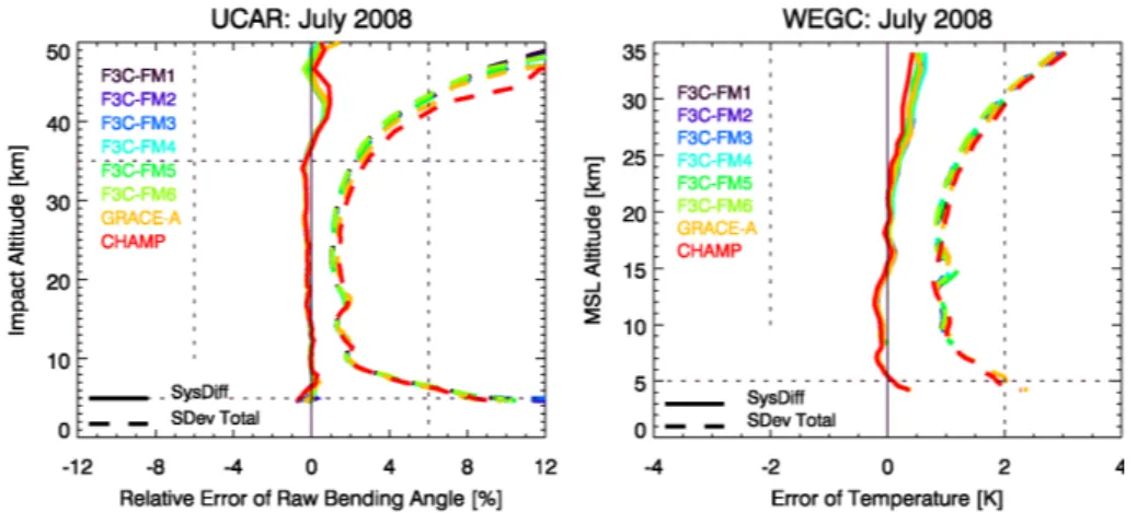
Fig. 1. RO minus ECMWF systematic difference (solid) and standard deviation (dashed) in July 2008 for UCAR raw bending angle (left panel) and WEGC dry temperature (right panel). Note different x- and y-axes of the two panels.
The statistics is calculated for different latitude regions (low, mid, and high latitudes, 30◦S to 30◦N, 30◦S/N to 60◦S/N, 60◦S/N to 90◦N/S, respectively, as well as for the global, Northern Hemisphere (NH), and Southern Hemi-sphere (SH) regions).
As an introductory example, Fig. 1 shows global mean UCAR raw bending angle (left panel) and WEGC dry tem-perature (right panel) systematic difference and standard de-viation relative to ECMWF in July 2008. As can be no-ticed from Fig. 1, data characteristics are very similar for all satellites. UCAR bending angle systematic difference is very close to zero between 9 km and 14 km, slightly negative up to about 37 km and positive above. Bending angle stan-dard deviation is within 2 % in the altitude range between 9 km and 32 km. Due to the smaller number of CHAMP and GRACE-A occultation events, standard deviation is slightly larger than for F3C. Maximum differences between CHAMP, GRACE-A, and F3C are observed above 35 km where devia-tions become larger than 0.5 %. Above about 42 km CHAMP raw bending angle observational error exceeds that of the other satellites by 1 %. This mainly derives from the larger bending angle noise observed in CHAMP data (Pirscher, 2010; Foelsche et al., 2011a).
WEGC dry temperature systematic difference is close to zero up to 24 km and positive above. Standard deviation does not exceed 2 K within 5 km and 30 km. CHAMP and GRACE-A standard deviations are up to 0.2 K larger than those of F3C.
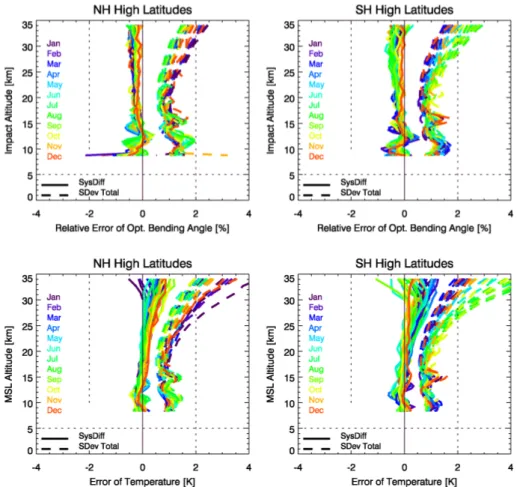
Figure 2 illustrates the temporal variation of the monthly statistics calculated for WEGC optimized bending angle (top panels) and dry temperature (bottom panels) for one single satellite (F3C/FM-1).
The systematic difference between RO and ECMWF bending angle is slightly negative during the whole time pe-riod, with differences being, in general, smaller than−0.5 %. Differences are slightly larger at high southern latitudes than at high northern latitudes. The temperature systematic
difference is very close to zero up to 20 km, increasing to about +1 K at 34 km.
Bending angle and temperature standard deviations show a clear seasonal variation above 20 km, where standard de-viation always increases in the winter hemisphere. This sea-sonal variation is somewhat more pronounced in the South-ern Hemisphere: bending angle standard deviations reach almost 3 % at high southern latitudes at 34 km in June, July, and August, temperature standard deviations become even larger than 4 K above 32 km in these particular winter months. These large errors might result from both RO data and ECMWF analysis profiles in roughly equal measure. RO retrieved data are affected by background data used for bend-ing angle initialization (for the reduction of bendbend-ing angle noise). Since the background does often not properly capture high latitude winter situations this may result in initializa-tion errors in such cases. However, ECMWF analysis fields also feature worst quality at high latitudes in the winter hemi-sphere, because there are only rather few good observational data available at high latitudes although a large number of ob-servations is crucial to capture high atmospheric variability.
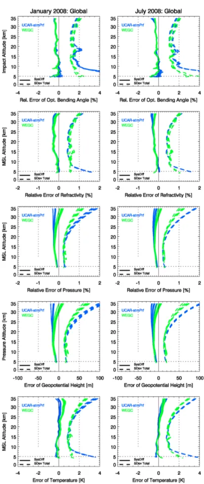
Figure 3 depicts differences between RO data retrieved at UCAR and at WEGC for different atmospheric parameters. At bending angle level (top panels), data are in very good agreement. The slightly larger standard deviation of UCAR data below 20 km results from the UCAR WO retrieval, which captures more (true) small-scale atmospheric variabil-ity than both, the WEGC GO retrieval and the ECMWF analyses.
Fig. 2. RO minus ECMWF systematic difference (solid) and standard deviation (dashed) for each month from January 2007 to Decem-ber 2009. Optimized bending angle (top panels) and dry temperature (bottom panels) statistics at high northern latitudes (left panels) and high southern latitudes (right panels) are shown for data retrieved at WEGC.
underestimates small-scale atmospheric variability, which explains the larger UCAR standard deviation relative to ECMWF. Since most of the background information en-ters the retrieval at high altitudes (>45 km), this difference cannot be observed in bending angle and refractivity below 35 km. However, it propagates down in the retrieval pro-cess through the hydrostatic integral (Rieder and Kirchen-gast, 2001a; Steiner and KirchenKirchen-gast, 2005). Near 34 km, the global UCAR dry pressure standard deviation is larger than the corresponding WEGC error by 0.8 %. UCAR dry geopotential height and dry temperature standard deviations are larger by about 50 m, and 0.7 K, respectively.
3.2 ECMWF model error
We use the global mean ECMWF temperature error as pro-vided by the ECMWF and made available from the ROPP 4.0 package (GRAS SAF, 2009). It is available at 91 vertical hy-brid levels up to a height of 80 km and is given in terms of standard deviation.
To estimate the error for atmospheric parameters other than temperature, we empirically derive conversion factors between the relevant standard deviations:
s1N/N[%] = cT2Ns1Tdry[K] (5)
s1α/α[%] = cN2αs1N/N[%] (6)
s1pdry/pdry[%] = cN2ps1N/N[%] (7)
s1Zdry[m] = cp2Zs1pdry/pdry[%]. (8)
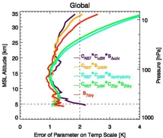
We findcT2N= 0.5 %/K,cN2α= 2.4 %/%,cN2p= 0.45 %/%,
and cp2Z= 65 m/%, where likewise the factors in
re-verse direction are cN2T = 1/cT2N= 2.0 K/%, cα2N=
1/cN2α= 0.42 %/%, cp2N= 1/cN2p= 2.2 %/%, and cZ2p=
1/cp2Z= 0.015 %/m, respectively. The latter are used in
Fig. 4. GRACE-A minus ECMWF standard deviation in Jan-uary 2008 shown for different atmospheric parameters, scaled to the same x-axis. The scaling factors, which are derived empirically, are given in the legend.
with theoretical and simulation studies of how RO errors propagate between retrieval steps from bending angle to dry temperature (Kursinski et al., 1997; Syndergaard, 1999; Rieder and Kirchengast, 2001a,b; Sofieva and Kyr¨ol¨a, 2004). Steiner et al. (2006) tested the sensitivity of the estimated L60 ECMWF refractivity error with respect to the temper-ature input for four different cases, where the tempertemper-ature standard deviation was multiplied by 1.0, 1.5, 2.0, and 2.5. They found that the results judged most reasonable for the case of doubling the ECMWF temperature standard devi-ation (2.0×T). However, our sensitivity tests yield the 1.5 case to be the most reasonable case. This reduction is attributable to the increase of the number of vertical levels from 60 to 91 and to the improved quality of ECMWF anal-ysis fields since 2006. Thus using data as of 2007 here, we estimate the ECMWF error to be 1.5×ECMWF standard de-viation as given by the ROPP 4.0 package (yielding 0.6 K at 5 km to 15 km, increasing to about 1 K at 35 km).
The ECMWF refractivity error is of the order of 0.3 % at 4 km to 15 km increasing to 0.5 % at 30 km, to 0.55 % at 35 km, and to 1.1 % at 50 km, which is slightly smaller than the findings of Kuo et al. (2004), who performed an estima-tion of short-range forecast errors using the Hollingsworth-L¨onnberg method.
We note that this ECMWF error is only a rough estimate, which does not reflect the true ECMWF error in regions with high atmospheric variability. Since the error does not vary with latitude and month, it might be too small at high lati-tudes during the winter season.
3.3 GPS RO observational error
The combined error scombined (see Sect. 3.1) contains the
RO observational error sobs and the ECMWF model error
sECMWF. The separation of these errors is performed by
sub-tracting the estimated ECMWF error from the combined er-ror in terms of variances
sobs = q
s2combined− sECMWF2 , (9)
which gives the observational error. It turns out that the esti-mated ECMWF error and the observational error are approx-imately of the same order of magnitude. A simple estimate of the observational errorsobsestcan thus be given by scaling
the combined error with 1/√2. This is a reasonable approxi-mation as can be seen in Fig. 5 and as was also found by Kuo et al. (2004) and Steiner et al. (2006).
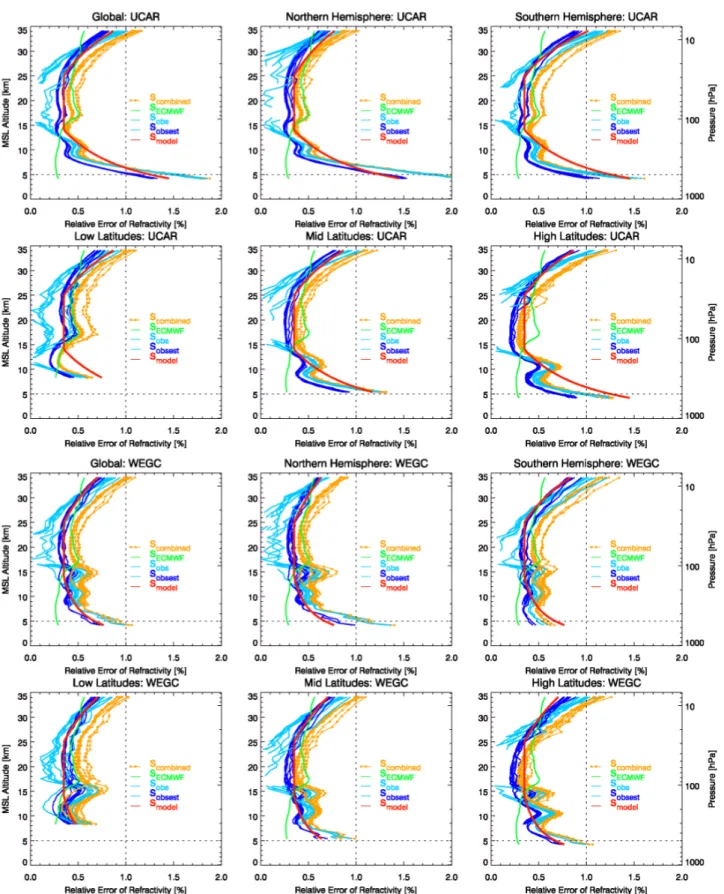
Figure 5 shows UCAR (top two rows) and WEGC (bottom two rows) refractivity error estimates in different geographi-cal regions in July 2008 including all four error types defined above (and in addition the error according to the simple ana-lytical model,smodel, discussed further below).
In the region where RO data are known to feature best quality (between 9 km and 25 km), the observational error sometimes becomes smaller than zero because the adopted (global static) ECMWF error is larger than the combined er-ror. In this region the estimated observational error amounts approximately to 0.3 %, which is in agreement with obser-vational errors found by Kuo et al. (2004). Below 9 km and above 25 km the observational error agrees well with the esti-mated observational error. The global mean observational er-ror in the lower stratosphere increases from≈0.3 % at 25 km to 0.9 % at 34 km. The increase is less in the (summer) Northern Hemisphere than in the (winter) Southern Hemi-sphere. Larger errors above 25 km are mainly attributable to the use of background data in bending angle retrieval as well as observational noise, which remains from uncalibrated ionospheric effects (Kursinski et al., 1997; Kuo et al., 2004). Below about 8 km the observational errors increase towards the surface mainly due to the complicated structure of humid-ity, superrefraction, oblique tangent point trajectories, and re-ceiver tracking errors (Foelsche and Kirchengast, 2004; Kuo et al., 2004; Foelsche et al., 2011b).
in all latitude regions. This error characteristic seems to be connected with the WEGC retrieval and related to the spe-cific handling of the degrading quality of the L2 signal in the lower atmosphere, which necessitates the extrapolation of the signal down into the troposphere (Steiner et al., 1999). In the WEGC OPSv5.4 scheme (and earlier versions) the top height of this extrapolation is set to a fixed impact height of 15 km, statistically increasing fractional errors immediately below, while in the UCAR scheme this height is set dynami-cally, according to the quality of the L2 signal. We note that this characteristic in the WEGC retrieval does not cause sys-tematic errors (see e.g. Fig. 2, where syssys-tematic differences of WEGC and UCAR to ECMWF do not differ), because the increased error behaves randomly from event to event. 3.4 GPS RO observational error model
Based on the above estimated observational errors we for-mulate a simple observational error model (indicated by the red lines in the panels of Fig. 5). This error model is derived from fitting simple analytical functions to the GPS RO ob-servational error. The vertical structure of the model follows Steiner and Kirchengast (2005) and Steiner et al. (2006). Their error modelsmodel as function of altitudezis
formu-lated as:
smodel =
s0 +q0
1 zb − zb1
Ttop
for 4 km < z ≤zTtop s0 forzTtop < z < zSbot s0 ·exp hz−zSbot
HS i
forzSbot ≤z < 50 km (10)
wherezTtop is the top level of the troposphere domain,zSbot
the bottom level of the stratosphere domain,s0is the error in
the upper troposphere/lower stratosphere domain,q0the best
fit parameter for the tropospheric model,bthe exponent, and HS the stratospheric error scale height. Note that the unit of
q0depends on the value ofb.
In addition to this vertical error model, we allocate a lati-tudinal and seasonal dependence in the form that any param-eterxcan be modeled as a function of latitudeϕand timeτ. This latitude and time dependence is formulated as
x(ϕ, τ ) = x0 +1x f (ϕ) g(τ, ϕ), (11)
wherex0is the basic mean magnitude of the parameter and
1xis the maximum amplitude of seasonal variations. The functionf (ϕ)accounts for latitudinal variations, the functiong(τ,ϕ)combines latitudinal and seasonal changes of atmospheric conditions:
f (ϕ) = max
0,min
|ϕ| − ϕ1xlo
ϕ1xhi −ϕ1xlo
,1
, (12)
g(τ, ϕ) =sign(ϕ)cos(2π τ ), (13)
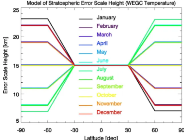
Fig. 6. Temperature stratospheric error scale height as a function of latitude for different months (different colors) as modeled by Eq. (15). with τ =
(m−1)−mlag
12 form∈ {1, ...,12} 3s−mlag
12 fors ∈ {1, ...,4}
(d−15)−30.5mlag
366 ford ∈ {1, ...,366}
. (14)
The functionf (ϕ)is zero at low latitudes (equatorwards of ϕ1xlo). Betweenϕ1xloandϕ1xhiit linearly increases to +1,
polewards ofϕ1xhi it is constant (+1) again. The function
g(τ, ϕ) yields always positive values in the winter hemi-sphere and negative values in the summer hemihemi-sphere. The model can be applied on a daily base withd being days of year, on a monthly base withm= 1 representing January and m= 12 being December, or on a seasonal base starting with s= 1 in March-April-May (MAM).
We apply Eq. (11) to the stratospheric error scale height 1HSused in Eq. (10), i.e. we setx0=HS0and1x=−1HS
and account by the latter parameter for larger/smaller obser-vational errors in the stratosphere at high latitudes during wintertime/summertime, where the error scale height thus needs to be smaller/larger. This results in
HS(ϕ, τ ) = HS0 −1HSf (ϕ) g(τ, ϕ). (15)
Forf (ϕ)we choseϕ1HSlo= 30◦andϕ1HShi= 60◦. Since the
annual cycle of atmospheric parameters does not show a tem-poral lag at high latitudes, we chosemlag= 0.
WEGC
αopt 14.0 km 25.0 km 0.8 % 10.0 % kmb 1.0 16.0 km 2.0 km
N,̺dry 14.0 km 25.0 km 0.35 % 2.5 % kmb 1.0 13.0 km 5.0 km
pdry 10.0 km 17.0 km 0.15 % 1.0 % kmb 0.5 10.0 km 4.0 km
Zdry 10.0 km 17.0 km 10.0 m 40.0 m kmb 0.5 10.0 km 4.0 km
Tdry 10.0 km 20.0 km 0.7 K 5.0 K kmb 0.5 15.0 km 8.0 km
scale height yields a stronger upward increase of observa-tional errors. Beside the extrema, two months always feature the same error scale height according to the cosine function (e.g. February and December, March and November...).
The error model given by Eqs. (10) and (15) depends on a few parameters only. Expressing the model in general par-lance, it exhibits the following simple height structure: the error is assumed to be constant around the tropopause region (a few kilometers below and above). Above this region it increases exponentially with the scale height of the error in-crease in the stratosphereHS. Below this region the error
in-creases closely proportional to an inverse height power-law. This functional behavior makes good physical sense as dis-cussed by Steiner and Kirchengast (2005). We fit observa-tional errors of all RO atmospheric parameters by the model of Eqs. (10) and (15). The most suitable parameter values for UCAR and WEGC data are summarized in Table 1.
Returning to Fig. 5 and comparing UCAR and WEGC re-fractivity observational errors it attracts attention that UCAR errors are distinctively larger in the lower troposphere. While UCAR errors increase from 0.3 % at 10 km to 1.5 % at 4 km, the increase in the WEGC data set is smaller: refractivity observational errors at 4 km generally remain smaller than 1.0 %. This is because the UCAR WO retrieval is able to cap-ture more small-scale atmospheric variability than ECMWF and WEGC (GO retrieval). The parametersq0andbare
ad-justed to account for this fact.
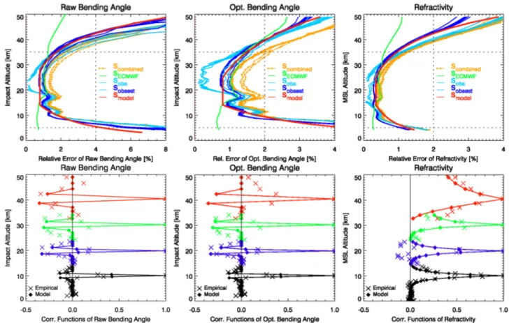
The error model is applicable up to 50 km for raw bend-ing angle, optimized bendbend-ing angle, and refractivity (up to 35 km for the other parameters). In addition, information on the error correlation structure is provided for these variables, for construction of error covariance matrices and their use,
e.g. in NWP assimilation systems. Figure 7 shows global er-ror estimates, erer-ror correlation functions and their models for UCAR raw and optimized bending angles, as well as refrac-tivity up to 50 km.
The impact of statistical optimization can clearly be seen comparing raw and optimized bending angle (Fig. 7, top panels). While the raw bending angle observational error exceeds 8 % near 45 km, the observational errors of the sta-tistically optimized bending angle and of refractivity remain smaller than 4 % up to 50 km (larger errors can occur in the lower troposphere). To account for the impact of background information at high altitudes, the observational error model for the optimized bending angle uses a lower zSbot and a
largerHS0and1HS.
The bottom panels of Fig. 7 show the empirical and mod-eled error correlation functions. Very good agreement with the results obtained by Steiner and Kirchengast (2005) is given and we follow their approach to model error correla-tions for raw bending angle by using a Mexican Hat function of the form.
S = Sij = si sj · 1 −
zi −zj
2
(c· L)2 !
· ˜f , (16)
whereSis the error covariance matrix with elementsSij,si
andsj are the standard deviations at height levelszi andzj,
Fig. 7.UCAR global error estimates (top panels) and error correlation functions (bottom panels) in July 2008 for raw and optimized bending angles as well as for refractivity up to 50 km. Empirical (x-symbols) and modeled (connected diamonds) correlation functions are shown based on GRACE-A data for four representative altitude levels from 10 km to 40 km.
any overshooting of error correlations that allows error cor-relation values to be negative), linearly decreasing toc= 0.8 at 50 km (stronger overshooting). The correlation lengthL was estimated to be 1.5 km at 50 km, linearly decreasing to 0.7 km at 14 km and kept at this value downwards. The er-ror correlation model obtained from raw bending angle data is also plotted for cross-check for the statistically optimized bending angle, which is generally not used for assimilation. The model almost perfectly fits also these data up to the 30 km level below which background information is neg-ligible, but above the influence of background information becomes noticeable through a much larger error correlation length and no overshooting. Error correlations at these alti-tude levels would require a different model such as, e.g. ap-plied for refractivity.
Refractivity error correlations are modeled after Steiner et al. (2006) using an exponential function of the form
S = Sij = si sj · exp −
zi −zj
L(z)
!
, (17)
where the correlation lengthL(z)was estimated to be 1 km up to 30 km altitude and then linearly increasing toL= 10 km
at 50 km. This increase accounts for an increasingly larger amount of background information at higher altitudes.
The error correlation functions are also usable for the WEGC data over their domain of availability up to 35 km.
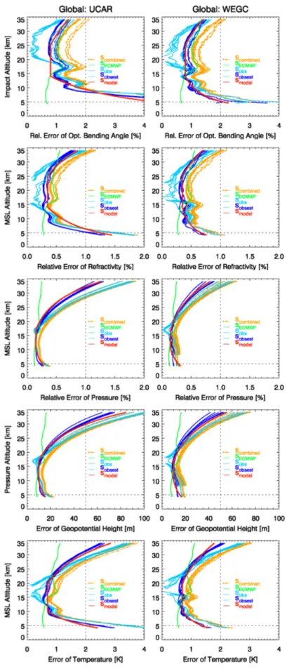
Figure 8 shows UCAR and WEGC observational errors and the corresponding simple error model for different at-mospheric parameters. Apart from the troposphere below 10 km, bending angle and refractivity observational errors are similar for both data sets; the observational error model is the same. However, pressure, geopotential height, and temperature observational errors are noticeably larger in the UCAR data set in the lower stratosphere. These larger UCAR observational errors are attributable to the NCAR climatol-ogy, which is used for bending angle initialization. This monthly mean climatology captures less atmospheric vari-ability than both ECMWF and WEGC, which results in larger observational errors due to downward propagation of initialization errors in the retrieval (hydrostatic integration) of pressure and further parameters. To account for these er-rors,HS, which is modeled utilizingHSand1HS, is smaller
4 Summary and conclusions
In this study, we presented results of an empirical error analy-sis of GPS radio occultation (RO) data. We analyzed RO pro-files of bending angle, refractivity, dry pressure, dry geopo-tential height, and dry temperature using data from CHAMP, GRACE-A, and Formosat-3/COSMIC (F3C). Comparing data processed at UCAR and at WEGC, we focused on the time period from January 2007 to December 2009.
In general, CHAMP, GRACE-A, and F3C data character-istics are in very good agreement. Global mean CHAMP and GRACE-A observational errors are only slightly larger than those of F3C, the differences being less than 0.3 % in bending angle, 0.1 % in refractivity, and 0.2 K in dry temper-ature at all altitude levels between 4 km and 35 km. Above about 35 km the CHAMP raw bending angle observational error increases stronger than that of GRACE-A and F3C. The difference exceeds 1 % above 42 km. Due to bending angle initialization at high altitudes, differences between the satellites above 35 km are smaller for other atmospheric pa-rameters. Observational errors for the different F3C satel-lites exhibit the same characteristics. Above≈20 km, the observational error shows a distinct seasonal dependence at high latitudes. Largest stratospheric errors are observed at high latitudes during wintertime, when atmospheric variabil-ity is most pronounced. These errors are mainly associated with background data used in the initialization for the re-duction of bending angle noise. The impact of background data used in the processing chain is also noticeable when comparing retrieval results from UCAR and WEGC. While UCAR uses a monthly NCAR climatology, WEGC utilizes co-located ECMWF forecast profiles for initialization. Since the monthly climatology significantly underestimates true at-mospheric variability, UCAR observational errors are larger than WEGC errors above≈20 km in dry pressure, dry geopo-tential height, and dry temperature. However, below 35 km these differences are not seen in bending angle and refrac-tivity. Larger UCAR bending angle observational errors be-low 20 km are attributable to the UCAR WO retrieval, which captures more (true) small-scale atmospheric variability than comparison data sets.
Based on the empirically derived error estimates we pro-vided a simple analytical model of the observational error for GPS RO atmospheric profiles of bending angle, refractivity, dry pressure, dry geopotential height, and dry temperature. Using the formulations introduced by Steiner and Kirchen-gast (2005) and Steiner et al. (2006) for the vertical error structure, we extended the model to also represent the lat-itudinal and seasonal dependencies of the observational er-ror. In the model a constant error is adopted around the tropopause region (a few kilometers above and below), which amounts to 0.8 % for bending angle, 0.35 % for refractivity, 0.15 % for dry pressure, 10 m for dry geopotential height, and to 0.7 K for dry temperature. Below this region the observa-tional error increases following an inverse height power-law.
Above this region the error increases exponentially with the latitudinal and seasonal behavior modeled through variation of the stratospheric error scale height.
The error correlation structure of bending angles follows a Mexican hat function including negative correlations while the error correlations of refractivity can be modeled by using a simple exponential function.
The observational error model is the same for UCAR and WEGC data but due to slightly different error characteristics below about 10 km and above about 20 km some parame-ter values had to be adjusted. Basically, the model is easily applicable in fields like operational meteorology or climate monitoring (see also Scherllin-Pirscher et al., 2011) and all parameter values in the model can be readily adjusted for in-dividual error characteristics of other RO data sets, e.g. from other processing chains than UCAR and WEGC.
The empirical estimates of the observational error from real data in this study were found somewhat larger, especially in the core domain from about 10 km to 20 km, than earlier error estimates based on theoretical and end-to-end simula-tion studies (Kursinski et al., 1997; Rieder and Kirchengast, 2001a; Steiner and Kirchengast, 2005). However, the empir-ical estimates are considered tentatively conservative, which is viewed as a good practice; more evidence and new valida-tion results in future may further refine the model. Overall the results underpin the high quality of RO data in the upper troposphere and lower stratosphere region.
Acknowledgements. We thank ECMWF (Reading, UK) for
providing analysis data. Furthermore we are grateful to the
UCAR/CDAAC and WEGC GPS RO operational team members, at WEGC especially to J. Fritzer and F. Ladst¨adter, for their contributions in OPS system development and operations. We also thank S. Sokolovskiy for helpful discussions. AKS was funded by the Austrian Science Fund (FWF) under grant P21642-N21 (TRENDEVAL project) and the work was also co-funded by grant P22293-N21 (BENCHCLIM project). WEGC OPS development was co-funded by ESA/ESTEC Noordwijk, ESA/ESRIN Frascati,
and FFG/ALR Austria. At UCAR the work was supported by
the National Science Foundation under Cooperative Agreement No. AGS-0918398/CSA No. AGS-0939962. The National Center for Atmospheric Research is also supported by the National Science Foundation.
M., K¨onig-Langlo, G., and Lauritsen, K. B.: Observa-tions and simulaObserva-tions of receiver-induced refractivity biases in GPS radio occultation, J. Geophys. Res., 111, D12101, doi:10.1029/2005JD006673, 2006.
Borsche, M., Kirchengast, G., and Foelsche, U.:
Tropi-cal tropopause climatology as observed with radio occul-tation measurements from CHAMP compared to ECMWF
and NCEP analyses, Geophys. Res. Lett., 34, L03702,
doi:10.1029/2006GL027918, 2007.
Chen, S.-Y., Huang, C.-Y., Kuo, Y.-H., and Sokolovskiy, S.: Ob-servational Error Estimation of FORMOSAT-3/COSMIC GPS Radio Occultation Data, Mon. Weather Rev., 139, 853–865, doi:10.1175/2010MWR3260.1, 2011.
Cucurull, L. and Derber, J. C.: Operational
implementa-tion of COSMIC observaimplementa-tions into NCEP’s global data
assimilation system, Weather Forecast., 23, 702–711,
doi:10.1175/2008WAF2007070.1, 2008.
Foelsche, U. and Kirchengast, G.: Sensitivity of GNSS radio occultation data to horizontal variability in the troposphere, Phys. Chem. Earth, 29, 225–240, doi:10.1016/j.pce.2004.01.007, 2004.
Foelsche, U., Borsche, M., Steiner, A. K., Gobiet, A., Pirscher, B., Kirchengast, G., Wickert, J., and Schmidt, T.: Observing up-per troposphere-lower stratosphere climate with radio occulta-tion data from the CHAMP satellite, Clim. Dynam., 31, 49–65, doi:10.1007/s00382-007-0337-7, 2008.
Foelsche, U., Scherllin-Pirscher, B., Ladst¨adter, F., Steiner, A. K., and Kirchengast, G.: Refractivity and temperature cli-mate records from multiple radio occultation satellites consis-tent within 0.05 %, Atmos. Meas. Tech. Discuss., 4, 1593–1615, doi:10.5194/amtd-4-1593-2011, 2011a.
Foelsche, U., Syndergaard, S., Fritzer, J., and Kirchengast, G.: Er-rors in GNSS radio occultation data: relevance of the measure-ment geometry and obliquity of profiles, Atmos. Meas. Tech., 4, 189–199, doi:10.5194/amt-4-189-2011, 2011b.
Gaspari, G. and Cohn, S. E.: Construction of correlation functions in two and three dimensions, Q. J. Roy. Meteorol. Soc., 125, 723–757, doi:10.1002/qj.49712555417, 1999.
Gobiet, A. and Kirchengast, G.: Advancements of Global Navi-gation Satellite System radio occultation retrieval in the upper stratosphere for optimal climate monitoring utility, J. Geophys. Res., 109, D24110, doi:10.1029/2004JD005117, 2004.
Gobiet, A., Kirchengast, G., Manney, G. L., Borsche, M., Retscher, C., and Stiller, G.: Retrieval of temperature profiles from
CHAMP for climate monitoring: intercomparison with
En-visat MIPAS and GOMOS and different atmospheric analyses,
Torre Juarez, M., and Yunck, T. P.: CHAMP and SAC-C at-mospheric occultation results and intercomparisons, J. Geophys. Res., 109, D06109, doi:10.1029/2003JD003909, 2004.
Healy, S.: Operational assimilation of GPS radio occultation mea-surements at ECMWF, ECMWF Newsletter, 111, 6–11, 2007. Healy, S. B. and Eyre, J. R.: Retrieving temperature, water vapour
and surface pressure information from refractive-index profiles derived by radio occultation: A simulation study, Q. J. Roy. Me-teorol. Soc., 126, 1661–1683, 2000.
Healy, S. B. and Th´epaut, J. N.: Assimilation experiments with CHAMP GPS radio occultation measurements, Q. J. Roy. Me-teorol. Soc., 132, 605–623, doi:10.1256/qj.04.182, 2006. Healy, S. B., Jupp, A. M., and Marquardt, C.: Forecast impact
ex-periment with GPS radio occultation measurements, Geophys. Res. Lett., 32, L03804, doi:10.1029/2004GL020806, 2005. Hedin, A. E.: Extension of the MSIS thermosphere model into the
middle and lower atmosphere, J. Geophys. Res., 96, 1159–1172, doi:10.1029/90JA02125, 1991.
Ho, S.-P., Kuo, Y.-H., Zeng, Z., and Peterson, T.: A comparison of lower stratospheric temperature from microwave measurements with CHAMP GPS RO data, Geophys. Res. Lett., 34, L15701, doi:10.1029/2007GL030202, 2007.
Ho, S.-P., Kirchengast, G., Leroy, S., Wickert, J., Mannucci, A. J., Steiner, A. K., Hunt, D., Schreiner, W., Sokolovskiy, S., Ao, C., Borsche, M., von Engeln, A., Foelsche, U., Heise, S., Iijima, B., Kuo, Y.-H., Kursinski, E. R., Pirscher, B., Ringer, M., Rocken, C., and Schmidt, T.: Estimating the uncertainty of using GPS radio occultation data for climate monitoring: Intercompari-son of CHAMP refractivity climate records from 2002 to 2006 from different data centers, J. Geophys. Res., 114, D23107, doi:10.1029/2009JD011969, 2009.
Jensen, A. S., Lohmann, M. S., Benzon, H.-H., and Nielsen, A. S.: Full spectrum inversion of radio occultation signals, Radio Sci., 38, 1040, doi:10.1029/2002RS002763, 2003.
Kuo, Y.-H., Sokolovskiy, S., Anthes, R. A., and Vandenberghe, F.: Assimilation of GPS radio occultation data for numerical weather prediction, Terrestrial, Atmos. Ocean. Sci., 11, 157–186, 2000.
Kuo, Y.-H., Wee, T.-K., Sokolovskiy, S., Rocken, C., Schreiner, W., Hunt, D., and Anthes, R. A.: Inversion and error estimation of GPS radio occultation data, J. Meteorol. Soc. Jpn., 82, 507–531, 2004.
Geophys. Res., 102, 23429–23465, 1997.
Leroy, S. S., Dykema, J. A., and Anderson, J. G.: Climate bench-marking using GNSS occultation, in: Atmosphere and Cli-mate: Studies by Occultation Methods, edited by: Foelsche, U., Kirchengast, G., and Steiner, A. K., Springer, Berlin, Heidelberg, 287–302, 2006.
Luntama, J.-P., Kirchengast, G., Borsche, M., Foelsche, U., Steiner, A., Healy, S. B., von Engeln, A., O’Clerigh, E., and Marquardt, C.: Prospects of the EPS GRAS mission for operational atmo-spheric applications, B. Am. Meteorol. Soc., 89, 1863–1875, doi:10.1175/2008BAMS2399.1, 2008.
Melbourne, W. G., Davis, E. S., Duncan, C. B., Hajj, G. A., Hardy, K. R., Kursinski, E. R., Meehan, T. K., Young, L. E., and Yunck, T. P.: The application of spaceborne GPS to atmospheric limb sounding and global change monitoring, JPL Publication, 94-18, 147, 1994.
Palmer, P. I. and Barnett, J. J.: Application of an optimal estima-tion inverse method to GPS/MET bending angle observaestima-tions, J. Geophys. Res., 106, 17147–17160, doi:10.1029/2001JD900205, 2001.
Palmer, P. I., Barnett, J. J., Eyre, J. R., and Healy, S. B.: A non-linear optimal estimation inverse method for radio occultation measurements of temperature, humidity, and surface pressure, J. Geophys. Res., 105, 17513–17526, doi:10.1029/2000JD900151, 2000.
Pirscher, B.: Multi-satellite climatologies of fundamental atmo-spheric variables from radio occultation and their validation (Ph.D. thesis), Wegener Center Verlag Graz, sci. Rep. 33-2010, 2010.
Pirscher, B., Foelsche, U., Borsche, M., Kirchengast, G., and Kuo, Y.-H.: Analysis of migrating diurnal tides detected in FORMOSAT-3/COSMIC temperature data, J. Geophys. Res., 115, D14108, doi:10.1029/2009JD013008, 2010.
Randel, W., Chanin, M. L., and Michaut, C.: SPARC intercompar-ison of middle atmosphere climatologies, WCRP 166, SPARC, WMO/TD No. 1142; SPARC Report No. 3, 2002.
Rennie, M. P.: The impact of GPS radio occultation assimilation at the Met Office, Q. J. Roy. Meteorol. Soc., 136, 116–131, doi:10.1002/qj.521, 2010.
Rieder, M. J. and Kirchengast, G.: Error analysis and characteri-zation of atmospheric profiles retrieved from GNSS occultation data, J. Geophys. Res., 106(D23), 31755–31770, 2001a. Rieder, M. J. and Kirchengast, G.: Error analysis for mesospheric
temperature profiling by absorptive occultation sensors, Ann. Geophys., 19, 71–81, doi:10.5194/angeo-19-71-2001, 2001b. Rocken, C., Anthes, R., Exner, M., Hunt, D., Sokolovskiy, S., Ware,
R., Gorbunov, M., Schreiner, W., Feng, D., Herman, B., Kuo, Y.-H., and Zuo, X.: Analysis and validation of GPS/MET data in the neutral atmosphere, J. Geophys. Res., 102, 29849–29866, 1997. Scherllin-Pirscher, B., Kirchengast, G., Steiner, A. K., Kuo, Y.-H., and Foelsche, U.: Quantifying uncertainty in climatologi-cal fields from GPS radio occultation: an empiriclimatologi-cal-analyticlimatologi-cal error model, Atmos. Meas. Tech. Discuss., 4, 2749–2788, doi:10.5194/amtd-4-2749-2011, 2011.
Schreiner, W., Rocken, C., Sokolovskiy, S., and Hunt, D.: Qual-ity assessment of COSMIC/FORMOSAT-3 GPS radio occul-tation data derived from single- and double-difference atmo-spheric excess phase processing, GPS Solutions, 14, 13–22, doi:10.1007/s10291-009-0132-5, 2009.
Sofieva, V. F. and Kyr¨ol¨a, E.: Abel integral inversion in occulta-tion measurements, in: Occultaocculta-tions for Probing Atmosphere and Climate, edited by: Kirchengast, G., Foelsche, U., and Steiner, A. K., Springer-Verlag, Berlin, Heidelberg, 77–86, 2004. Sokolovskiy, S. and Hunt, D.: Statistical optimization approach
for GPS/MET data inversion, paper presented at the URSI GPS/MET workshop, 1996.
Steiner, A. K. and Kirchengast, G.: Ensemble-based analysis of errors in atmospheric profiles retrieved from GNSS occultation data, in: Occultations for Probing Atmosphere and Climate, edited by: Kirchengast, G., Foelsche, U., and Steiner, A. K., Springer-Verlag, Berlin, Heidelberg, 149–160, 2004.
Steiner, A. K. and Kirchengast, G.: Error analysis of GNSS radio occultation data based on ensembles of profiles from end-to-end simulations, J. Geophys. Res., 110, D15307, doi:10.1029/2004JD005251, 2005.
Steiner, A. K., Kirchengast, G., and Ladreiter, H. P.: Inversion, er-ror analysis, and validation of GPS/MET occultation data, Ann. Geophys., 17, 122–138, doi:10.1007/s00585-999-0122-5, 1999. Steiner, A. K., L¨oscher, A., and Kirchengast, G.: Error
characteris-tics of refractivity profiles retrieved from CHAMP radio occul-tation data, in: Atmosphere and Climate: Studies by Occuloccul-tation Methods, edited by: Foelsche, U., Kirchengast, G., and Steiner, A. K., Springer-Verlag, Berlin, Heidelberg, 27–36, 2006. Steiner, A. K., Kirchengast, G., Lackner, B. C., Pirscher, B.,
Borsche, M., and Foelsche, U.: Atmospheric temperature change detection with GPS radio occultation 1995 to 2008, Geophys. Res. Lett., 36, L18702, doi:10.1029/2009GL039777, 2009. Syndergaard, S.: Retrieval analysis and methodologies in
atmo-spheric limb sounding using the GNSS radio occultation tech-nique, Danish Meteorological Institute, Copenhagen, Denmark, 1999.
Wickert, J., Schmidt, T., Michalak, G., Heise, S., Arras, C., Beyerle, G., Falck, C., K¨onig, R., Pingel, D., and Rothacher, M.: GPS radio occultation with CHAMP, GRACE-A, SAC-C, TerraSAR-X, and FORMOSAT-3/COSMIC: Brief review of results from GFZ, in: New Horizons in Occultation Research: Studies in At-mosphere and Climate, edited by: Steiner, A. K., Pirscher, B., Foelsche, U., and Kirchengast, G., Springer-Verlag, Berlin, Hei-delberg, 3–16, 2009.