Generation of a Bending Angle Radio Occultation Climatology (BAROCLIM) and its use in radio occultation retrievals

(1)

AMTD

7, 8193–8231, 2014

Generation of BAROCLIM and its use in RO retrievals

B. Scherllin-Pirscher et al.

Title Page

Abstract Introduction

Conclusions References

Tables Figures

◭ ◮

Back Close

Full Screen / Esc

Printer-friendly Version Interactive Discussion

Discussion

P

a

per

|

Discus

sion

P

a

per

|

Discussion

P

a

per

|

Discussion

P

a

per

|

Atmos. Meas. Tech. Discuss., 7, 8193–8231, 2014 www.atmos-meas-tech-discuss.net/7/8193/2014/ doi:10.5194/amtd-7-8193-2014

This discussion paper is/has been under review for the journal Atmospheric Measurement Techniques (AMT). Please refer to the corresponding final paper in AMT if available.

Generation of a Bending Angle Radio

Occultation Climatology (BAROCLIM) and

its use in radio occultation retrievals

B. Scherllin-Pirscher1, S. Syndergaard2, U. Foelsche1, and K. B. Lauritsen2

1

Wegener Center for Climate and Global Change (WEGC) and Institute for Geophysics, Astrophysics, and Meteorology/Institute of Physics (IGAM/IP), University of Graz, Graz, Austria

2

Danish Meteorological Institute, Copenhagen, Denmark

Received: 24 July 2014 – Accepted: 25 July 2014 – Published: 8 August 2014

Correspondence to: B. Scherllin-Pirscher (barbara.pirscher@uni-graz.at)

(2)

AMTD

7, 8193–8231, 2014

Title Page

Tables Figures

◭ ◮

Back Close

Full Screen / Esc

Discussion

P

a

per

|

Discus

sion

P

a

per

|

Discussion

P

a

per

|

Discussion

P

a

per

|

Abstract

In this paper, we introduce a bending angle radio occultation climatology (BAROCLIM) based on Formosat-3/COSMIC (F3C) data. This climatology represents the monthly-mean atmospheric state from 2006 to 2012. Bending angles from radio occultation (RO) measurements are obtained from the accumulation of the change in the

ray-5

path direction of Global Positioning System (GPS) signals. Best quality of these near-vertical profiles is found from the middle troposphere up to the mesosphere. Beside RO bending angles we also use data from the Mass Spectrometer and Incoherent Scatter Radar (MSIS) model to expand BAROCLIM in a spectral model, which (theoretically) reaches from the surface up to infinity. Due to the very high quality of BAROCLIM up to

10

the mesosphere, it can be used to detect deficiencies in current state-of-the-art anal-ysis and reanalanal-ysis products from numerical weather prediction (NWP) centers. For bending angles derived from European Centre for Medium-Range Weather Forecasts (ECMWF) analysis fields from 2006 to 2012, e.g., we find a positive bias of 0.5 % to 1 % at 40 km, which increases to more than 2 % at 50 km. BAROCLIM can also be used

15

as a priori information in RO profile retrievals. In contrast to other a priori information (i.e., MSIS) we find that the use of BAROCLIM better preserves the mean of raw RO measurements. Global statistics of statistically optimized bending angle and refractivity profiles also confirm that BAROCLIM outperforms MSIS. These results clearly demon-strate the utility of BAROCLIM.

20

1 Introduction

Global data sets of the lower and middle atmosphere (troposphere to upper meso-sphere) provide important information to understand atmospheric dynamics of the Earth’s climate system. Observational data as well as analysis/reanalysis data and atmospheric models are used, e.g., to study specific atmospheric phenomena such

25

(3)

AMTD

7, 8193–8231, 2014

Title Page

Tables Figures

◭ ◮

Back Close

Full Screen / Esc

Discussion

P

a

per

|

Discus

sion

P

a

per

|

Discussion

P

a

per

|

Discussion

P

a

per

|

Oscillation) (e.g., Angell, 1981; Scherllin-Pirscher et al., 2012), or the QBO (Quasi Bi-ennial Oscillation) (e.g., Baldwin et al., 2001). Long-term observational records, reanal-ysis data sets, and atmospheric models can also be used to investigate atmospheric climate change (IPCC, 2013).

Simple empirical atmospheric models are of high utility if a quick but reasonable

5

estimate of the atmospheric state is of main interest. This is of importance, e.g., for simulation studies in the field of atmospheric remote sensing or within the retrieval of atmospheric parameters from remote sensing measurements. For this purpose several research communities use early empirical models like CIRA (Committee on Space Research (COSPAR), International Reference Atmosphere) (Fleming et al., 1990) or

10

Mass Spectrometer and Incoherent Scatter Radar (MSIS) (Hedin, 1991; Picone et al., 2002).

Published in the early sixties, the CIRA model was the earliest comprehensive clima-tological model of the atmosphere, which contains information up to the thermosphere. This model is based on observational data like radiosondes, rocket data, and

satel-15

lite observations. Its fourth version CIRA-86 includes thermosphere models as well as tables of monthly-mean zonal-mean temperature, pressure, geopotential height, and zonal wind from the surface to an altitude of 120 km. The most recent CIRA version (CIRA-2012) contains updated versions of empirical models of the Earth’s upper atmo-sphere (above 120 km) (CIRA, 2012).

20

Recent MSIS model versions (MSIS-90 and NRLMSIS-00) provide information on atmospheric composition, total mass density, and temperature from the ground up to the exosphere also using observations from ground, rockets, and satellites. The MSIS model output depends on time (day of year, universal time, local solar time), location (altitude, latitude, longitude), geomagnetic activity (represented by the magnetic index

25

Ap), and solar activity (represented by the 10.7 cm solar radiation flux,F10.7).

(4)

AMTD

7, 8193–8231, 2014

Title Page

Tables Figures

◭ ◮

Back Close

Full Screen / Esc

Discussion

P

a

per

|

Discus

sion

P

a

per

|

Discussion

P

a

per

|

Discussion

P

a

per

|

middle-atmosphere climatologies from approximately 10 km to 80 km including histor-ical measurements from rocketsonde winds and temperatures (1970 to 1989), lidar temperature data (1990s), global meteorological analyses, and satellite data and found notable differences between these data sets. Some biases found in atmospheric anal-yses were caused by the low vertical resolution of these data as well as the low vertical

5

resolution of some assimilated satellite measurements.

Since 2004 research initiatives tried to understand and eliminate errors of previous middle atmosphere models, building new, state-of-the-art analysis and reanalysis prod-ucts. However, there are still uncertainties and differences in current reanalysis prod-ucts, and the SPARC (Stratosphere-troposphere Processes And their Role in Climate)

10

Reanalysis/analysis Intercomparison Project (S-RIP, Fujiwara et al., 2012) aims at understanding and reasonably interpreting these differences and contributing to future reanalysis improvements in the middle atmosphere.

In this study, we aim at compiling and investigating a global climatological model from recent high resolution radio occultation (RO) bending angles. The RO method

15

(Melbourne et al., 1994; Kursinski et al., 1997) is an active limb sounding technique, which utilizes radio signals continuously broadcast by Global Positioning System (GPS) satellites. The measured quantity is the phase change of the GPS signal as a func-tion of time, which is a measure for physical atmospheric parameters, in particular bending angle and radio refractivity, from which density, pressure, geopotential height,

20

temperature, and humidity profiles can be derived with very high accuracy (though in the lower moist troposphere auxiliary information is necessary to separate dry air and moist air contributions to the refractivity). Precise and stable oscillators aboard the GPS satellites ensure measurement stability and consistency between various RO missions, without the need for instrument dependent calibrations (Hajj et al., 2004;

25

Schreiner et al., 2007; Foelsche et al., 2011).

(5)

AMTD

7, 8193–8231, 2014

Title Page

Tables Figures

◭ ◮

Back Close

Full Screen / Esc

Discussion

P

a

per

|

Discus

sion

P

a

per

|

Discussion

P

a

per

|

Discussion

P

a

per

|

CHAMP RO measurements from 2001 to 2008 are supplemented with measure-ments from SAC-C (launched in 2000), GRACE (2002), Metop-A (2006), TerraSAR-X (2007), C/NOFS (2008), OceanSat-2 (2009), Tandem-X (2010), SAC-D (2011), Megha-Tropiques (2011), Metop-B (2012), FY-3C (2013), and KOMPSAT-5 (2013) as well as from the first six-satellite RO constellation Formosat-3/COSMIC (F3C; launched in

5

2006).

Atmospheric profiles from RO are used for data assimilation in numerical weather prediction (NWP) (e.g., Healy and Thépaut, 2006; Cucurull and Derber, 2008), and in atmospheric and climate research (see Anthes, 2011; Steiner et al., 2011, for re-views). Most studies utilize RO profiles in the upper troposphere and lower stratosphere

10

(UTLS) region, i.e., the altitude range from approximately 5 km to 35 km, where RO pro-files of pressure, geopotential height, and temperature are known to be of best quality (Scherllin-Pirscher et al., 2011b).

The top altitude of RO measurements depends on the instrument settings, but is at least 80 km (e.g., Metop-A and Metop-B). For F3C it is usually about 120 km or

15

higher. However, at these altitudes, individual RO profiles are dominated by measure-ment noise and ionospheric disturbances, because neutral atmospheric density gra-dients are small. To derive refractivity profiles via the Abel integral transform (Fjeldbo et al., 1971), and since noisy and erroneous information from high altitudes propagates downwards in the retrieval process, bending angles are combined with a priori

informa-20

tion, e.g., from a climatology, usually applying statistical optimization (Rodgers, 2000; Healy, 2001; Gorbunov, 2002; Gobiet and Kirchengast, 2004; Lohmann, 2005).

Formally, the upper limit in the Abel integral transform is infinity (Fjeldbo et al., 1971). If a climatology is used for statistical optimization, it is therefore necessary that it is able to provide a good measure of the bending angle to very high altitudes. Usually, the

25

(6)

AMTD

7, 8193–8231, 2014

Title Page

Tables Figures

◭ ◮

Back Close

Full Screen / Esc

Discussion

P

a

per

|

Discus

sion

P

a

per

|

Discussion

P

a

per

|

Discussion

P

a

per

|

of derived atmospheric profiles (Ho et al., 2012; Steiner et al., 2013). Therefore high quality a priori information is of particular importance.

Ao et al. (2012) and Gleisner and Healy (2013) introduced a new approach to derive GPS RO climatological products. Instead of averaging individual refractivity profiles, they calculated monthly-mean bending angles and computed mean refractivity as the

5

Abel inversion of the mean bending angle. Ao et al. (2012) showed that the maximum altitude through which the F3C measurements are useful increased substantially, which leads to a reduced bias in climatological averages of refractivity. The main drawback of this approach, however, is that it can only be used to obtain mean atmospheric fields and is not applicable to individual RO profiles.

10

The generation of the bending angle radio occultation climatology (BAROCLIM) de-scribed in this paper is mainly based on the work by Foelsche and Scherllin-Pirscher (2012) and Scherllin-Pirscher (2013). Section 2 gives a detailed description of the RO data set as well as of reference data used in this study. In Sect. 3 we present the method used to construct BAROCLIM and in Sect. 4 we discuss potential

system-15

atic errors and evaluate the model by comparing it to reference data from NWP anal-ysis fields provided by the European Centre for Medium-Range Weather Forecasts (ECMWF). In Sect. 5 we show that BAROCLIM can further be used as a priori in-formation for statistical optimization in RO profile retrievals. Conclusions are drawn in Sect. 6.

20

2 Data

For the generation of BAROCLIM, we used ionosphere-corrected bending angles as a function of impact altitude (impact parameter with the local radius of curvature and geoid undulation subtracted). These profiles were retrieved with the Wegener Center for Climate and Global Change (WEGC) Occultation Processing System version 5.6

25

(7)

AMTD

7, 8193–8231, 2014

Title Page

Tables Figures

◭ ◮

Back Close

Full Screen / Esc

Discussion

P

a

per

|

Discus

sion

P

a

per

|

Discussion

P

a

per

|

Discussion

P

a

per

|

Input data to the WEGC processing system are profiles of excess phase and am-plitude as well as precise orbit information of GPS and low Earth orbit (LEO) satel-lites (level 1a data) provided by other data centers. Currently WEGC uses level 1a data provided by University Corporation for Atmospheric Research (UCAR)/COSMIC Data Analysis and Archive Center (CDAAC) for all RO satellite missions. Since recent

5

UCAR/CDAAC processing versions vary for different missions and GPS receivers used for RO measurements are not of the same quality (Foelsche et al., 2011, e.g., found different bending angle noise for different missions), we decided to use only data from the F3C constellation. The UCAR/CDAAC processing version of F3C data used in this study was 2010.2640 for the whole time period starting in 2006.

10

The processing system at UCAR/CDAAC relies on the Bernese software package to obtain precise orbits of F3C satellites and applies single differencing to remove F3C clock offsets (Schreiner et al., 2009). In their inversion retrieval, WEGC first corrects GPS and LEO orbits for the Earth’s oblateness (Syndergaard, 1998), removes outliers from L1 and L2 excess phase profiles, and smooths data with a regularization filter

15

(Syndergaard, 1999). Doppler shift profiles are then calculated from excess phase pro-files via numerical di_fferentiation. In the upper troposphere and above, bending an-gles are computed from Doppler shift profiles based on geometric optics (Melbourne et al., 1994). Wave optics retrieval is applied in the lower and middle troposphere (Gor-bunov, 2002; Gorbunov et al., 2004; Gorbunov and Lauritsen, 2004). To remove the

20

ionospheric contribution to the bending angle, WEGC applies ionospheric correction on bending angle level following Vorob’ev and Krasil’nikova (1994) and Hocke et al. (2003). Except from the use of F3C open-loop data (Sokolovskiy et al., 2006) and the wave optics retrieval in the lower and middle troposphere, the WEGC OPSv5.6 bending angle retrieval is very similar to the OPSv5.4 processing described by Ho et al. (2012)

25

and Steiner et al. (2013).

(8)

AMTD

7, 8193–8231, 2014

Title Page

Tables Figures

◭ ◮

Back Close

Full Screen / Esc

Discussion

P

a

per

|

Discus

sion

P

a

per

|

Discussion

P

a

per

|

Discussion

P

a

per

|

orbit altitude because solar panels were stuck, which limited the power and payload operation of this spacecraft). From 2007 to 2009 F3C always tracked more than 60 000 RO events per month (exception: June 2009, UCAR/CDAAC provided approximately 55 000 level 1a profiles). Since 2010 the number of measurements decreased again due to battery degradation of all spacecraft. Furthermore, F3C/FM-3 has been out of

5

contact since 1 August 2010. However, the minimum number of level 1a data provided by UCAR/CDAAC per month in the period between 2006 and 2012 was always larger than 30 000.

Since RO profiles usually do not reach higher than about 120 km (only about 80 km for Metop) and because the true neutral atmospheric bending angle decreases nearly

10

exponentially with height (and therefore measurement noise dominates in a fractional sense in the mesosphere and above), there is an upper limit to which RO data are useful for the generation of a climatology. To extend BAROCLIM to higher altitudes we used bending angles based on a modified version of the MSIS-90 empirical model of the neutral atmosphere (Hedin, 1991). Høeg et al. (1995) modified the original MSIS-90

15

model by smoothing out a discontinuity at 72.5 km, and fixing the local apparent solar time at 0 h, the solar radio flux at F10.7=150×10−

22

W m−1Hz−1, and the magnetic index atAp=4.

Subsequently, this modified version of the MSIS model was used to generate spec-tral models of refractivity and bending angle for the use of fast and efficient modeling

20

and inversion of RO data. The spectral model of refractivity,N, was obtained from the MSIS pressure,p, and temperature,T (N=77.6p/T), for the 15th of every month. The spectral model of bending angle was obtained from the spectral refractivity model via the Abel integral transform. Thus, the MSIS-based bending angles and refractivities contain no information on atmospheric humidity and are given as a function of month,

25

(9)

AMTD

7, 8193–8231, 2014

Title Page

Tables Figures

◭ ◮

Back Close

Full Screen / Esc

Discussion

P

a

per

|

Discus

sion

P

a

per

|

Discussion

P

a

per

|

Discussion

P

a

per

|

Generic Occultation Performance Simulator (EGOPS) (Fritzer et al., 2012) and the Ra-dio Occultation Processing Package (ROPP) (Culverwell, 2013).

To validate BAROCLIM we used operational ECMWF analysis fields at T42 horizon-tal resolution (comparable to RO horizonhorizon-tal resolution) and 91 vertical levels. Profiles were extracted at mean RO event location of those F3C measurements, which were

5

used to construct BAROCLIM. We applied a forward model to derive ECMWF bending angles from refractivity.

We will show in Sect. 5 that BAROCLIM can be used as a priori information for the statistical optimization in the processing of RO measurements. To investigate the per-formance of BAROCLIM as a priori information, we used level 1a data from CHAMP,

10

GRACE-A, SAC-C, and F3C from January 2008 and July 2008 (level 1a data were again provided by UCAR/CDAAC; CHAMP data version was 2009.2650, other satel-lites had consistent data version 2010.2640) and applied the WEGC OPSv5.6 retrieval using BAROCLIM and MSIS as a priori information for bending angle initialization. Re-trieved atmospheric profiles were then compared to operationally reRe-trieved OPSv5.6

15

profiles, which used ECMWF short-range forecasts as a priori in the statistical opti-mization (Schwärz et al., 2013).

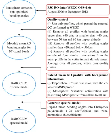
3 BAROCLIM generation

Figure 1 summarizes the steps of the BAROCLIM generation. Using ionosphere-corrected bending angles as a function of impact altitude on a regular 200 m grid, we

20

first applied a quality control (QC) to identify and exclude bad profiles before averaging bending angles in latitude and altitude and calculating monthly-mean 10◦ zonal-mean bending angles. These long-term monthly means include data from 6 or 7 years. Since we aimed at generating a BAROCLIM spectral model, which (theoretically) reaches from the surface to infinity, we extended mean RO profiles with MSIS. We refer to these

25

(10)

AMTD

7, 8193–8231, 2014

Title Page

Tables Figures

◭ ◮

Back Close

Full Screen / Esc

Discussion

P

a

per

|

Discus

sion

P

a

per

|

Discussion

P

a

per

|

Discussion

P

a

per

|

was then constructed by expansion into Chebychev polynomials and zonal harmonics. Below we describe these steps in detail.

3.1 Quality control of individual profiles

Bending angles, which are very noisy and/or contain unphysical values, can strongly affect the quality of a bending angle climatology. To avoid entering these profiles in

5

BAROCLIM, we only used OPSv5.6 profiles, which passed the external QC performed at WEGC (Schwärz et al., 2013). This external QC comprises bending angle, refractiv-ity, and temperature profiles, which are compared to co-located profiles from ECMWF analysis fields. The profile is flagged bad if the difference between the RO and the ECMWF profile is larger than 20 % in bending angle, 10 % in refractivity, and/or 25 K

10

in temperature. However, since these quality checks are only performed in the upper troposphere and lower stratosphere region up to 35 km, profiles passing the external QC can still be very noisy in the upper stratosphere and above.

The inspection of individual bending angle profiles indeed revealed that it is imper-ative to perform an additional QC. We therefore introduced a threefold approach for

15

an additional outlier rejection. In a first step we rejected all profiles with bending an-gles smaller than₋40 µrad or larger than +40 µrad in the altitude range from 50 km to 80 km. In this altitude range, neutral atmospheric bending angles are usually smaller than 20 µrad and bending angles smaller/larger than±40 µrad result from very strong (unphysical) noise, possibly sometimes related to ionospheric scintillations (Zeng and

20

Sokolovskiy, 2010).

To also detect very bad profiles below 50 km, we rejected all profiles with bending an-gles smaller than₋20 µrad below 50 km in a second step. Profiles, which were flagged bad by these QC mechanisms were outlier profiles, which could damage the quality of BAROCLIM.

25

(11)

AMTD

7, 8193–8231, 2014

Title Page

Tables Figures

◭ ◮

Back Close

Full Screen / Esc

Discussion

P

a

per

|

Discus

sion

P

a

per

|

Discussion

P

a

per

|

Discussion

P

a

per

|

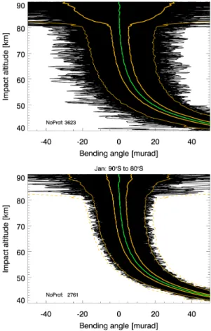
deviations for 10◦ latitude bands for long-term monthly means, and rejected all pro-files with bending angles outside of four standard deviations (4σ) from the mean in the altitude range from the surface to 100 km. Figure 2 shows F3C profiles for the month of January before and after application of this 4σ-criterion. This figure reveals that ap-plication of this final QC results in a considerable decrease in standard deviation.

5

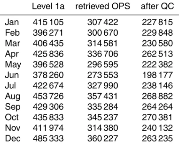
Table 1 gives an overview on the number of profiles provided by UCAR/CDAAC, re-trieved at WEGC, and passing BAROCLIM QC. The number of bending angle profiles for a given month used to generate BAROCLIM is always larger than 200 000, ex-cept for June, when it is slightly below. In some months, however, the number is even larger than 260 000. These numbers are large enough and su_fficient to obtain a smooth

10

BAROCLIM up to about 60 km.

3.2 Average over high quality profiles

The optimal horizontal extent of the regions to calculate a typical climatological mean from high quality measurements is a trade-o_ff between a su_fficiently large number of profiles and atmospheric variability. Our experience of building atmospheric

climatolo-15

gies utilizing RO data (e.g., Foelsche et al., 2008; Scherllin-Pirscher et al., 2011a) showed that 10◦ zonal bands were a reasonable choice for calculating mean atmo-spheric profiles from RO data. These bands range from 90◦S to 90◦N resulting in 18 zonal bands.

The mean number of profiles per 10◦latitudinal band varied between 11 000 (June)

20

and 15 000 (October). However, the latitudinal distribution of RO events is not uni-form, which is due to the orbit characteristics of the GPS and F3C satellites (orbit inclinations of 55◦ and 72◦, respectively). The largest number of RO measurements per latitude band is obtained at mid-latitudes, where more than 20 000 profiles enter BAROCLIM. A smaller number of measurements per latitude band is obtained at low

25

(12)

AMTD

7, 8193–8231, 2014

Title Page

Tables Figures

◭ ◮

Back Close

Full Screen / Esc

Discussion

P

a

per

|

Discus

sion

P

a

per

|

Discussion

P

a

per

|

Discussion

P

a

per

|

2000 high-latitude profiles to be sufficient due to the decrease of zonal surface area with increasing latitude. Thus, 2000 profiles are enough to represent a small area.

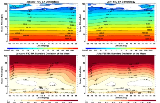
Long-term monthly-mean bending angles for 10◦ zonal bands for January and July are shown in Fig. 3 together with their standard error of the mean σmean=σ/

√

N (σ

is the standard deviation andN is here the number of observations used to estimate

5

the mean – not to be confused with refractivity). Bending angles are negative (white areas) somewhat above an altitude of 80 km, and the standard error of the mean is larger than 10 % above 70 km in the winter hemisphere at high latitudes. While negative mean bending angles might be caused by residual systematic ionospheric errors (see Danzer et al., 2013), the high standard error of the mean (in a fractional sense) is

10

a result of the decreasing bending angle with altitude. Below 60 km to 70 km, however, mean bending angles are rather smooth and the standard error of the mean generally does not exceed 2 %.

3.3 BAROCLIM discrete model

Because of the generally decreasing bending angle with altitude the mean bending

an-15

gle (Fig. 3) is error dominated above 80 km. Therefore we combined the mean bend-ing angles with a priori information to generate a model that is useful also above the mesosphere. A priori information profiles can be obtained from already existing clima-tological models or profile data sets. Current state-of-the-art analysis, reanalysis, or forecast products from NWP centers do not reach high enough in the atmosphere (the

20

ECMWF model top, e.g., is at 0.01 hPa corresponding approximately to 80 km) and can therefore not be used for extension to higher altitudes.

Since already readily available, we decided to use the modified MSIS climatology as a priori information. In order to make maximum use of the information content of the RO data, and since the MSIS-90 climatology might be biased at high altitudes, we

25

(13)

AMTD

7, 8193–8231, 2014

Title Page

Tables Figures

◭ ◮

Back Close

Full Screen / Esc

Discussion

P

a

per

|

Discus

sion

P

a

per

|

Discussion

P

a

per

|

Discussion

P

a

per

|

January to December, and found the best match to the RO data using a least squares fit to the RO mean bending angle profile in the altitude range from 60 km to 80 km, where RO data quality is still high. To correct remaining background biases, the best-fitting MSIS profile was then multiplied with a fit factor obtained from regression with respect to the mean RO bending angle profile at high altitudes (least-squares adjustment from

5

60 km to 80 km). We found fit coefficients being close to unity (0.99 to 1.01) with only exceptions in Southern Hemisphere winter at high latitudes (80◦S to 90◦S), where fit coefficients were as small as 0.96, 0.88, and 0.91 in May, June, and July, respectively. To combine the mean RO bending angle profile with the corresponding MSIS pro-file, we applied statistical optimization by inverse covariance weighting (Gobiet and

10

Kirchengast, 2004) between 60 km and 80 km using an error correlation length of 2 km for the RO profile and an error correlation length of 15 km for the adjusted MSIS model profile. Furthermore, we assumed the MSIS background error to increase linearly from 0 % at 80 km to 15 % at 78 km, kept it constant at 15 % between 78 km and 62 km and then increased linearly again from 15 % at 62 km to 100 % at 60 km. All these

per-15

cent values refer to the absolute values of the MSIS bending angle at the respective impact altitude level. The observational error was set to the mean background error be-tween 62 km and 78 km and was constant with height (in absolute value, not percentage wise). Using these settings we obtained smooth statistically optimized bending angles, for which the height where the retrieval to a priori error ratio (Gobiet et al., 2007) equals

20

50 % is 67.2 km for all profiles. Outside of the transition region from 60 km to 80 km, the statistically optimized bending angle equals that of MSIS (above 80 km) or that of the mean RO profiles (below 60 km).

Even though Fig. 3 indicates that the mean bending angles reach down to the surface (2 km impact altitude approximately corresponds to 0 km altitude), mean bending angle

25

(14)

AMTD

7, 8193–8231, 2014

Title Page

Tables Figures

◭ ◮

Back Close

Full Screen / Esc

Discussion

P

a

per

|

Discus

sion

P

a

per

|

Discussion

P

a

per

|

Discussion

P

a

per

|

individual profiles (even if profiles are tracked all the way to the surface) depends on the bending angle. For the ray grazing the surface in one occultation event with a large bending angle, the impact altitude is larger than for the ray grazing the surface in an-other occultation event with smaller bending angle. It thus becomes dubious to talk about bending angle at the lowest impact altitude for the mean profile.

5

Being aware that MSIS is a dry air climatology (no humidity is included in this model) and accepting that BAROCLIM will not reflect real atmosphere conditions at the lowest altitudes, we decided to use this model for extending BAROCLIM down to the surface. BAROCLIM is therefore, like MSIS, a dry air model, being clearly wrong in regions were moisture is usually abundant, but for technical reasons smooth bending angles in the

10

lower troposphere close to the surface are necessary when generating the BAROCLIM spectral model.

To extend mean RO bending angles down to the surface, we first extracted the MSIS profile for the given month and latitude and searched for the best fit in longitude. We then applied a cosine transition with the mean RO bending angle. Since the amount

15

of water vapor in the lower troposphere depends on latitude, we performed RO-MSIS transition between 5 km and 10 km from 60◦S/N to 90◦S/N, between 7 km and 12 km from 30◦S/N to 60◦S/N, and between 10 km and 15 km from 30◦S to 30◦N.

To sum up, our BAROCLIM discrete model is available for every month (January to December), has a horizontal resolution of 10◦-zonal bands, and a vertical gridding of

20

200 m. It relies 100 % on RO data from the upper troposphere up to 60 km. Above 80 km and below 5, 7, or 10 km (depending on latitude), it consists of data-driven adjusted MSIS profiles.

3.4 BAROCLIM spectral model

For fast and easy access to BAROCLIM at any latitude and impact altitude, and to

25

(15)

AMTD

7, 8193–8231, 2014

Title Page

Tables Figures

◭ ◮

Back Close

Full Screen / Esc

Discussion

P

a

per

|

Discus

sion

P

a

per

|

Discussion

P

a

per

|

Discussion

P

a

per

|

structured than the smooth, almost exponentially decreasing bending angle, we ex-panded a function into Chebychev polynomials, which depends on the bending angle scale height.

First we introduced the variablez=h−hsurf (z≥0), wherehis impact altitude and

h_surf is the lowest possible impact altitude corresponding to a hypothetical ray grazing

5

the surface. The lowest impact altitude was estimated from the MSIS climatology using

hsurf=N MSIS surf 10

−6

RE, where RE=6371 km is the mean radius of the Earth andN MSIS surf

is MSIS refractivity at the surface extracted at the specific month and latitude and at longitudeλ=0◦. The bending angle α(z) was then extracted from the BAROCLIM discrete model by interpolation to a number of discrete impact heights evaluatingz(x)=

10

100(ln 2−ln(1−x)) atkmaxvalues ofxgiven byxk=cos(π(k−12)/kmax) (k=1,. . .,kmax).

This mapping yields a finer vertical spacing at low altitudes and coarser vertical spacing at higher altitudes. Having α(z) at these discrete impact heights, the bending angle scale heightHS(z) was calculated as

HS(z)=

z

ln αsurf/α(z)

, (1)

15

whereαsurf is the bending angle atz=0 (also extracted from the BAROCLIM discrete

model).

Chebychev coefficients,cj, were obtained from

cj =

2

kmax

k_max

X

k=1

G(xk) cos

π(j−1) k−12

kmax

!

, (2)

20

where

G(x)₌HS(z(x))−(m z(x)+b), (3)

and m and b are slope and intercept of a straight line fit to the scale height at high

25

altitudes. Finally,j=1,. . .,kmaxandkmaxis the number of extracted Chebychev coeffi

(16)

AMTD

7, 8193–8231, 2014

Title Page

Tables Figures

◭ ◮

Back Close

Full Screen / Esc

Discussion

P

a

per

|

Discus

sion

P

a

per

|

Discussion

P

a

per

|

Discussion

P

a

per

|

The Chebychev coefficients were then expanded into zonal harmonics. Besides the Chebychev coefficients, alsohsurf,αsurf,m, andbwere expanded into zonal harmonics.

In general, zonal harmonics coefficientsA_n are obtained from a given functionf(y), where normallyy=cosθ(θis co-latitude (polar distance)) as (see e.g., Spiegel, 1979)

A_n=2n+1

2

+1 Z

−1

f(y)P_n(y) dy, (4)

5

where Pn are Legendre Polynomials, n=1,. . .,nmax, and nmax is the number of

ex-tracted zonal harmonics coefficients. In our case f(y) was eithercj,hsurf,αsurf,m, or

b. Thus, the final output of the BAROCLIM spectral model wasnmaxzonal harmonics

coefficients of kmax Chebychev coefficients, surface impact altitude, surface bending

10

angle, and slope and intercept of the straight line.

To reconstruct the bending angle from the BAROCLIM spectral model for a given im-pact altitude and latitude, we first applied Clenshaw’s recurrence formula (Press et al., 1986) for zonal harmonics to obtain the Chebychev coefficientscj as well ashsurf,αsurf,

m, andb. We also applied Clenshaw’s recurrence formula to reconstructG(x) (where

15

x=1₋2 exp(₋z/100)) before reconstructing bending angles using

α(z)₌αsurfexp

− z

HS(z)

. (5)

More details on the expansion of BAROCLIM into Chebychev polynomials and zonal harmonics as well as their reconstruction can be found in Scherllin-Pirscher (2013).

20

To settle on the order of the Chebychev polynomials and the degree of the zonal har-monics, we calculated differences between the bending angles from the BAROCLIM discrete model and the BAROCLIM spectral model for different choices of kmax and

nmaxaiming at minimizing these differences. Since the BAROCLIM discrete model has

a horizontal resolution of 10◦-zonal bands (18 zonal bands), we found minimum

dif-25

(17)

AMTD

7, 8193–8231, 2014

Title Page

Tables Figures

◭ ◮

Back Close

Full Screen / Esc

Discussion

P

a

per

|

Discus

sion

P

a

per

|

Discussion

P

a

per

|

Discussion

P

a

per

|

polynomials we found reasonable good agreement between the BAROCLIM discrete model and the BAROCLIM spectral model for 64 Chebychev coefficients. When us-ing 128 Chebychev coefficients the spectral model even reproduces the sharp tropical tropopause. For this reason we decided to use 128 Chebychev coefficients when re-constructing the bending angle, but lower vertical resolution bending angles can be

5

reconstructed using a smaller number of Chebychev coefficients. This could be use-ful for applications where computational speed is more important than high vertical resolution.

Figure 4 shows (as an example for the month of January) the BAROCLIM spectral model for 128 Chebychev coefficients and 18 zonal harmonics coefficients. The left

10

right panel of Fig. 4 shows that di_fferences between the BAROCLIM discrete model and the BAROCLIM spectral model are, in general, within 0.5 % up to 60 km (a closer inspection of the differences reveals that it is even within 0.3 % in most places). Larger di_fferences are found close to the 60 km altitude level (transition height of RO-only data and statistically optimized RO data) and above 80 km where the absolute amount of the

15

bending angle is so small that even very small differences yield a noticeable percentage value.

4 Evaluation of BAROCLIM

4.1 Error sources

Atmospheric climatological fields of RO data are affected by (i) random

statisti-20

cal errors, (ii) systematic errors, and (iii) sampling errors (Scherllin-Pirscher et al., 2011a). Random statistical errors include, e.g., receiver thermal noise, clock stabil-ity/differencing errors, ionospheric noise, and statistical velocity errors (see e.g., Ram-sauer and Kirchengast, 2001). Random statistical errors diminish by averaging over a large number of profiles. Since BAROCLIM is based on a very large number of quality

(18)

AMTD

7, 8193–8231, 2014

Title Page

Tables Figures

◭ ◮

Back Close

Full Screen / Esc

Discussion

P

a

per

|

Discus

sion

P

a

per

|

Discussion

P

a

per

|

Discussion

P

a

per

|

controlled RO soundings, all contributions from statistical errors are negligible, except at the highest altitudes (cf. Fig. 3).

Systematic errors are more important for BAROCLIM. From the RO measurement and retrieval perspective, these errors include systematic errors in orbit determination, local multipath, residual ionospheric errors, and errors due to assumptions in the RO

5

retrieval. Systematic errors of BAROCLIM also include contributions due to the addi-tional use of MSIS at high and low altitudes.

Schreiner et al. (2009) investigated the uncertainty of UCAR/CDAAC precise orbit determination (POD) of F3C satellites and found a velocity error of 0.17 mm s−1, which approximately corresponds to an F3C bending angle error of 0.05 µrad (1 % at 60 km).

10

Due to the lack of an alternative measurement system onboard of F3C, Schreiner et al. (2009) could not give an estimate of the orbit accuracy. If we assume that half of the F3C velocity error is attributable to a systematic error component, the corresponding BAROCLIM error will be 0.5 % at 60 km.

Errors due to local multipath depend on the spacecraft size and on the reflection

15

coefficient (Rocken et al., 2008). For F3C these local multipath errors are estimated to be smaller than 0.05 mm s−1 (Rocken et al., 2008), which corresponds to 0.015 µrad in bending angle when using velocity error to bending angle error conversion given by Schreiner et al. (2009). This error corresponds to 0.3 % at 60 km.

Systematic residual ionospheric errors are important for BAROCLIM. In general,

20

ionospheric residual errors depend on the level of ionization at high altitudes, which again depends on local time (i.e., day- versus nighttime conditions due to solar insola-tion) as well as on solar activity (Kursinski et al., 1997; Schreiner et al., 2011; Danzer et al., 2013). Danzer et al. (2013) showed that this error rarely exceeds 0.1 µrad from mid 2006 to end of 2011. When averaging over this time period, it is even smaller than

25

(19)

AMTD

7, 8193–8231, 2014

Title Page

Tables Figures

◭ ◮

Back Close

Full Screen / Esc

Discussion

P

a

per

|

Discus

sion

P

a

per

|

Discussion

P

a

per

|

Discussion

P

a

per

|

Systematic errors due to assumptions in the retrieval process (such as spherical symmetry) are assumed to be small at high altitudes (Rocken et al., 2008).

Another BAROCLIM systematic error component results from the additional use of the MSIS model at low (tropospheric) and high (mesospheric and above) altitudes. Large systematic BAROCLIM errors in the troposphere are due to the absence of

at-5

mospheric water vapor in the MSIS model. For this reason BAROCLIM is not generally useful for tropospheric studies. Systematic errors from MSIS a priori information used at high altitudes (below 70 km) are assumed to be small due to the way MSIS was used (finding a bending angle profile that fits the mean RO data at high altitudes).

Finally, errors in BAROCLIM are caused by discrete sampling times and locations of

10

RO measurements (sampling error, see e.g., Foelsche et al., 2008; Scherllin-Pirscher et al., 2011a). The sampling error depends on the number of profiles and atmospheric variability and can be estimated from reference data that reflect true spatial and tem-poral variability. Using 6 to 7 years of RO data for BAROCLIM with more than 200 000 profiles per month (exception: June with 198 177 profiles), the BAROCLIM sampling

15

error is negligible.

4.2 Comparison to ECMWF

In December 2006 ECMWF started assimilating RO data in its operational assimila-tion system (Healy, 2007), which implies that ECMWF analyses and RO measure-ment data are not independent anymore. Healy et al. (2005) and Healy and Thépaut

20

(2006) showed that assimilation of RO data significantly improved the forecast skill of the ECMWF operational system in the upper troposphere and lower stratosphere. Foelsche et al. (2009) found reduced biases in mean ECMWF analysis fields at least up to 30 km after ECMWF started assimilating RO. However, even though the assimila-tion is performed up to 50 km (von Engeln et al., 2009), a large RO observaassimila-tional error

25

(20)

AMTD

7, 8193–8231, 2014

Title Page

Tables Figures

◭ ◮

Back Close

Full Screen / Esc

Discussion

P

a

per

|

Discus

sion

P

a

per

|

Discussion

P

a

per

|

Discussion

P

a

per

|

analysis profiles therefore do not only provide valuable information about the quality of BAROCLIM but also on the quality of ECMWF analyses, especially at high altitudes.

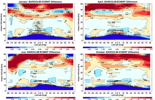
Figure 5 shows that the differences are small (<0.5 %) in the upper troposphere and lower stratosphere region between approximately 10 km and 35 km. Besides this good agreement, striking features, which are very similar in all months are (i) large negative

5

differences in the troposphere, (ii) a band of positive differences (mostly<1 %) above approximately 35 km, and (iii) large positive differences (>2 %) above 50 km.

Large negative tropospheric differences are caused by BAROCLIM being a dry air model. Neglecting atmospheric humidity yields unrealistically small bending angles in regions where humidity is high. Positive BAROCLIM minus ECMWF analysis diff

er-10

ences above 35 km (<1 %) and above 50 km (>2 %) are most likely attributable to bi-ases in ECMWF analyses rather than to BAROCLIM. This hypothesis is supported by comparisons of MIPAS (Michelson Interferometer for Passive Atmospheric Sounding onboard the European environmental satellite ENVISAT) and MLS (Microwave Limb Sounder onboard the US Aura satellite) measurements, which consistently show

neg-15

ative MIPAS/MLS minus ECMWF temperature differences above approximately 2 hPa (Chauhan et al., 2009). A negative temperature bias corresponds to a positive refractiv-ity bias, which in turn corresponds to a positive bending angle bias (see e.g., Scherllin-Pirscher et al., 2011b) as shown in Fig. 5.

This comparison clearly shows that BAROCLIM is of very high quality at least up to

20

60 km and has the potential to validate middle-atmosphere data.

5 Use of BAROCLIM in RO profile retrievals

The intended aim of BAROCLIM was its use as a priori information in RO profile re-trievals. We therefore evaluated its performance by processing occultation data from different RO missions and comparing retrieved atmospheric profiles obtained with

dif-25

(21)

AMTD

7, 8193–8231, 2014

Title Page

Tables Figures

◭ ◮

Back Close

Full Screen / Esc

Discussion

P

a

per

|

Discus

sion

P

a

per

|

Discussion

P

a

per

|

Discussion

P

a

per

|

As mentioned in Sect. 2, we used level 1a RO data provided by UCAR/CDAAC for all missions and applied the WEGC OPSv5.6 retrieval to obtain ionosphere-corrected bending angles. As bending angle a priori information for statistical optimization we used BAROCLIM and MSIS profiles co-located to RO events (termed “BAROCLIM-Col” and “MSIS-“BAROCLIM-Col”, respectively) and BAROCLIM and MSIS profiles, which best fit

5

the ionosphecorrected bending angle (termed “BAROCLIM-SF” and “MSIS-SF”, re-spectively, where SF means “searched” and “fit”). This best-fit algorithm was similar to the “enhanced IGAM high-altitude retrieval scheme” described by Gobiet and Kirchen-gast (2004), searching for the best-fitting MSIS/BAROCLIM profile between 35 km and 55 km and performing linear regression to find a multiplication factor to refine the fit to

10

the data from 45 km to 65 km. For comparison, we also included operationally retrieved OPSv5.6 profiles (Schwärz et al., 2013), which use ECMWF short-range forecasts as a priori information (termed “OPSv5.6”).

To assess the performance of BAROCLIM in RO profile retrievals we calculated monthly statistics of raw ionosphere-corrected bending angles minus optimized

bend-15

ing angles. Since the purpose of statistical optimization is to reduce random errors, while preserving the mean, the mean di_fference between raw and optimized bending angles is an indicator of the quality of the background climatology.

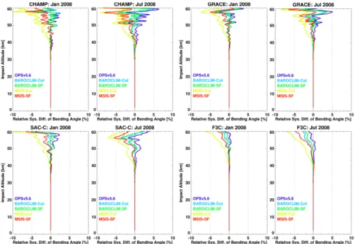
Figure 6 shows mean results for January and July 2008 for CHAMP, GRACE-A, SAC-C, and F3C. Since noise of individual ionosphere-corrected raw bending angle

20

profiles is high in the middle and upper stratosphere, difference profiles have a very large standard deviation. We did not include this information in the plot but note that it reaches approximately 15 % between 45 km (CHAMP) and 50 km (F3C).

Figure 6 shows that while bending angle systematic differences of BAROCLIM-SF, BAROCLIM-Col, and OPSv5.6 are very close to zero for all satellites and both months,

25

(22)

AMTD

7, 8193–8231, 2014

Title Page

Tables Figures

◭ ◮

Back Close

Full Screen / Esc

Discussion

P

a

per

|

Discus

sion

P

a

per

|

Discussion

P

a

per

|

Discussion

P

a

per

|

Figure 7 shows how differences propagate from statistically optimized bending angle to refractivity using either MSIS-SF, BAROCLIM-SF, or OPSv5.6. Since bending angle and refractivity differences shown in Fig. 7 are calculated against ECMWF analyses, zero difference does not necessarily mean that it is close to the truth (cf. Fig. 5 and the discussion there about). Bending angle and refractivity systematic differences are very

5

similar for all satellites with differences amongst the satellites being, in general, smaller than 1.5 % up to 60 km. Comparison of the three methods reveals distinctively larger differences in bending angle and refractivity. While BAROCLIM-SF profiles are close to operationally retrieved OPSv5.6 profiles in the entire altitude range, MSIS-SF clearly performs worse compared to the other methods. Difference between MSIS-SF and

10

ECMWF profiles reaches 3 % at approximately 55 km in bending angle and refractivity. Contrary to systematic differences, the magnitude of the standard deviation features distinct satellite dependent characteristics. Since CHAMP data noise is larger com-pared to the other satellites, OPS uses more weight of the a priori information, which results in smoother profiles and smaller standard deviation above 40 km. When

com-15

paring standard deviations of the three methods, larger standard deviations are found for the two search and fit algorithms than for OPSv5.6.

6 Summary, conclusions, and outlook

In this study, we used radio occultation (RO) data from the Formosat-3/COSMIC (F3C) mission from August 2006 to December 2012 (more than 6 years of data) to compile

20

a bending angle radio occultation climatology (BAROCLIM). After careful quality con-trol we calculated “long-term” monthly means for 10◦-zonal bands from the surface up to 100 km. Since mean RO profiles become more noisy above 60 km (in a fractional sense) and are error dominated above 80 km, we used a priori information from the Mass Spectrometer and Incoherent Scatter Radar (MSIS) climatology and applied

sta-25

(23)

AMTD

7, 8193–8231, 2014

Title Page

Tables Figures

◭ ◮

Back Close

Full Screen / Esc

Discussion

P

a

per

|

Discus

sion

P

a

per

|

Discussion

P

a

per

|

Discussion

P

a

per

|

and performed a cosine transition to mean RO profiles in the middle troposphere. This implies that BAROCLIM is a dry air model in the troposphere. However, BAROCLIM re-lies on RO data from the upper troposphere up to 60 km and also contains RO-derived information higher up.

We showed that BAROCLIM is of very high quality in the stratosphere and lower

5

mesosphere, where systematic biases are small. In this altitude range differences between BAROCLIM and ECMWF (European Centre for Medium-Range Weather Forecasts) analyses (forward modeled to bending angle) rather show deficiencies in ECMWF analyses than in BAROCLIM. At 40 km, e.g., we find BAROCLIM minus ECMWF analysis bending angle differences of about 0.5 % to 1.0 % and sometimes

10

more. Above 50 km, this di_fference even exceeds 2 %. This is generally consistent with findings by Chauhan et al. (2009), using other types of satellite measurements.

A main application of BAROCLIM is its use as a priori information in RO profile re-trievals. We evaluated BAROCLIM by comparing retrieved RO profiles initialized with different a priori information provided by BAROCLIM, MSIS, and ECMWF. These

com-15

parisons showed that RO bending angles initialized with BAROCLIM are close to raw (un-optimized) bending angles. This means that BAROCLIM-initialized bending angles preserve the mean of the raw measurements, while MSIS-initialized bending angles are slightly negatively biased. Comparison of retrieved RO profiles to ECMWF anal-yses also indicated that BAROCLIM outperforms MSIS. These results confirmed the

20

capability of BAROCLIM to be used in RO profile retrievals.

The main advantage of BAROCLIM compared to the average bending angle ap-proach proposed by Ao et al. (2012) and Gleisner and Healy (2013) is that utilization of BAROCLIM yields individual RO profiles rather than climatological fields and individual RO profiles are known to provide accurate information of, e.g., tropopause

characteris-25

(24)

AMTD

7, 8193–8231, 2014

Title Page

Tables Figures

◭ ◮

Back Close

Full Screen / Esc

Discussion

P

a

per

|

Discus

sion

P

a

per

|

Discussion

P

a

per

|

Discussion

P

a

per

|

Our current BAROCLIM spectral model does not include profiles of particular atmo-sphere conditions arising, e.g., during and after sudden stratospheric warmings (SSW). Since several major and minor SSW events occurred since 2006 it is possible to include such profiles in BAROCLIM. Another BAROCLIM update could comprise its inversion to refractivity, density, pressure, and temperature so that these parameters could be

5

used for other applications as well.

Acknowledgements. We want to thank Gottfried Kirchengast (WEGC) for valuable scientific discussions. We are also grateful to UCAR/CDAAC for the provision of level 1a RO data and WEGC for the provision of level 1b RO data. Special thanks to M. Schwärz and J. Fritzer (WEGC) for the contributions in OPS system development and operations. Furthermore, we 10

thank ECMWF (Reading, UK) for providing analysis data. B. Scherllin-Pirscher and U. Foelsche were partly funded by GRAS SAF (visiting scientist project VS14) and ROM SAF (visiting scientist project VS19), and by the Austrian Science Fund (FWF) under grants P22293-N21 (BENCHCLIM) and T620-N29 (DYNOCC). S. Syndergaard and K. B. Lauritsen have been sup-ported by the ROM SAF (Radio Occultation Meteorology Satellite Application Facility) which is 15

an operational RO processing center under EUMETSAT.

References

AIAA: Guide to Reference and Standard Atmosphere Models, ANSI/AIAA G-003B-2004, Amer-ican Institute of Aeronautics and Astronautics, 2004. 8195

Angell, J. K.: Comparison of variations in atmospheric quantities with sea surface temperature 20

variations in the equatorial eastern Pacific, Mon. Weather Rev., 109, 230–243, 1981. 8195 Anthes, R. A.: Exploring Earth’s atmosphere with radio occultation: contributions to weather,

climate and space weather, Atmos. Meas. Tech., 4, 1077–1103, doi:10.5194/amt-4-1077-2011, 2011. 8197

Anthes, R. A., Bernhardt, P. A., Chen, Y., Cucurull, L., Dymond, K. F., Ector, D., Healy, S. B., 25

(25)

COSMIC/FORMOSAT-AMTD

7, 8193–8231, 2014

Title Page

Tables Figures

◭ ◮

Back Close

Full Screen / Esc

Discussion

P

a

per

|

Discus

sion

P

a

per

|

Discussion

P

a

per

|

Discussion

P

a

per

|

3 mission: early results, B. Am. Meteorol. Soc., 89, 313–333, doi:10.1175/BAMS-89-3-313, 2008. 8205

Ao, C. O., Mannucci, A. J., and Kursinski, E. R.: Improving GPS radio occultation strato-spheric refractivity retrievals for climate benchmarking, Geophys. Res. Lett., 39, L12701, doi:10.1029/2012GL051720, 2012. 8198, 8215

5

Baldwin, M. P., Gray, L. J., Dunkerton, T. J., Hamilton, K., Haynes, P. H., Randel, W. J., Holton, J. R., Alexander, M. J., Hirota, I., Horinouchi, T., Jones, D. B. A., Kinnersley, J. S., Marquardt, C., Sato, K., and Takahashi, M.: The quasi-biennial oscillation, Rev. Geophys., 39, 179–229, 2001. 8195

Chauhan, S., Höpfner, M., Stiller, G. P., von Clarmann, T., Funke, B., Glatthor, N., Grabowski, U., 10

Linden, A., Kellmann, S., Milz, M., Steck, T., Fischer, H., Froidevaux, L., Lambert, A., San-tee, M. L., Schwartz, M., Read, W. G., and Livesey, N. J.: MIPAS reduced spectral res-olution UTLS-1 mode measurements of temperature, O₃, HNO₃, N₂O, H₂O and relative humidity over ice: retrievals and comparison to MLS, Atmos. Meas. Tech., 2, 337–353, doi:10.5194/amt-2-337-2009, 2009. 8212, 8215

15

CIRA: COSPAR International Reference Atmosphere–2012, CIRA-2012, Models of the Earth’s Upper Atmosphere, Technical report, chapters 1 to 3, CIRA, available at: http://spaceweather.usu.edu/files/uploads/PDF/COSPAR_INTERNATIONAL_REFERENCE_ ATMOSPHERE-CHAPTER-1_3%28rev-01-11-08-2012%29.pdf (last access: July 2014), 2012. 8195

20

Cucurull, L. and Derber, J. C.: Operational implementation of COSMIC observa-tions into NCEP’s global data assimilation system, Weather Forecast., 23, 702–711, doi:10.1175/2008WAF2007070.1, 2008. 8197

Culverwell, I.: The Radio Occultation Processing Package (ROPP) – An Overview, Version 7.0 (ROPP-7 v7.0), ROM SAF CDOP-2, ROM SAF, Ref: SAF/ROM/METO/UG/ROPP/001, July 25

2013, available at: http://www.romsaf.org (last access: July 2014), 2013. 8201

Danzer, J., Scherllin-Pirscher, B., and Foelsche, U.: Systematic residual ionospheric errors in radio occultation data and a potential way to minimize them, Atmos. Meas. Tech., 6, 2169– 2179, doi:10.5194/amt-6-2169-2013, 2013. 8204, 8210

Fjeldbo, G., Kliore, A. J., and Eshleman, V. R.: The neutral atmosphere of Venus as studied with 30

(26)

AMTD

7, 8193–8231, 2014

Title Page

Tables Figures

◭ ◮

Back Close

Full Screen / Esc

Discussion

P

a

per

|

Discus

sion

P

a

per

|

Discussion

P

a

per

|

Discussion

P

a

per

|

Fleming, E. L., Chandra, S., Barnett, J. J., and Corney, M.: Zonal mean temperature, pressure, zonal wind, and geopotential height as functions of latitude, COSPAR International Refer-ence Atmosphere: 1986, Part II: Middle Atmosphere Models, Adv. Space Res., 10, 11–59, 1990. 8195

Foelsche, U. and Scherllin-Pirscher, B.: Development of bending angle climatology from RO 5

data, CDOP visiting scientist report 14, GRAS SAF, Ref: SAF/GRAS/DMI/REP/VS14/001, July 2012, available at: http://www.romsaf.org (last access: July 2014), 2012. 8198

Foelsche, U., Borsche, M., Steiner, A. K., Gobiet, A., Pirscher, B., Kirchengast, G., Wickert, J., and Schmidt, T.: Observing upper troposphere-lower stratosphere climate with radio occul-tation data from the CHAMP satellite, Clim. Dynam., 31, 49–65, doi:10.1007/s00382-007-10

0337-7, 2008. 8203, 8211

Foelsche, U., Pirscher, B., Borsche, M., Steiner, A. K., Kirchengast, G., and Rocken, C.: Climatologies based on radio occultation data from CHAMP and Formosat-3/COSMIC, in: New Horizons in Occultation Research: Studies in Atmosphere and Climate, edited by: Steiner, A. K., Pirscher, B., Foelsche, U., and Kirchengast, G., Springer, 181–194, 15

doi:10.1007/978-3-642-00321-9_15, 2009. 8211

Foelsche, U., Scherllin-Pirscher, B., Ladstädter, F., Steiner, A. K., and Kirchengast, G.: Re-fractivity and temperature climate records from multiple radio occultation satellites consis-tent within 0.05 %, Atmos. Meas. Tech., 4, 2007–2018, doi:10.5194/amt-4-2007-2011, 2011. 8196, 8199

20

Fritzer, J., Kirchengast, G., and Pock, M.: EGOPS 5.6/DDD, End-to-End Generic Occultation Performance Simulation and Processing System Version 5.6 (EGOPS 5.6)/Detailed De-sign Document, WEGC-IGAM/UniGraz technical report for ESA/ESTEC no. 2/2012, doc-id: WEGC-EGOPS-2012-TR-02, issue 1.1, WEGC and IGAM, 2012. 8201

Fujiwara, M., Polavarapu, S., and Jackson, D.: A proposal of the SPARC reanalysis/analysis 25

intercomparison project, SPARC Newsletter, 38, 14–17, 2012. 8196

Gleisner, H. and Healy, S. B.: A simplified approach for generating GNSS radio occultation re-fractivity climatologies, Atmos. Meas. Tech., 6, 121–129, doi:10.5194/amt-6-121-2013, 2013. 8198, 8215

Gobiet, A. and Kirchengast, G.: Advancements of Global Navigation Satellite System radio oc-30

(27)

AMTD

7, 8193–8231, 2014

Title Page

Tables Figures

◭ ◮

Back Close

Full Screen / Esc

Discussion

P

a

per

|

Discus

sion

P

a

per

|

Discussion

P

a

per

|

Discussion

P

a

per

|

Gobiet, A., Kirchengast, G., Manney, G. L., Borsche, M., Retscher, C., and Stiller, G.: Retrieval of temperature profiles from CHAMP for climate monitoring: intercomparison with Envisat MIPAS and GOMOS and different atmospheric analyses, Atmos. Chem. Phys., 7, 3519– 3536, doi:10.5194/acp-7-3519-2007, 2007. 8205

Gorbunov, M. E.: Canonical transform method for processing radio occultation data in the lower 5

troposphere, Radio Sci., 37, 1076, doi:10.1029/2000RS002592, 2002. 8197, 8199

Gorbunov, M. E. and Lauritsen, K. B.: Analysis of wave fields by Fourier integral operators and their application for radio occultations, Radio Sci., 39, RS4010, doi:10.1029/2003RS002971, 2004. 8199

Gorbunov, M. E., Benzon, H.-H., Jensen, A. S., Lohmann, M. S., and Nielsen, A. S.: Compara-10

tive analysis of radio occultation processing approaches based on Fourier integral operators, Radio Sci., 39, RS6004, doi:10.1029/2003RS002916, 2004. 8199

Hajj, G. A., Ao, C. O., Iijima, B. A., Kuang, D., Kursinski, E. R., Mannucci, A. J., Mee-han, T. K., Romans, L. J., de la Torre Juarez, M., and Yunck, T. P.: CHAMP and SAC-C atmospheric occultation results and intercomparisons, J. Geophys. Res., 109, D06109, 15

doi:10.1029/2003JD003909, 2004. 8196

Healy, S.: Operational assimilation of GPS radio occultation measurements at ECMWF, ECMWF Newsletter, 111, 6–11, 2007. 8211

Healy, S. B.: Radio occultation bending angle and impact parameter errors caused by horizontal refractive index gradients in the troposphere: a simulation study, J. Geophys. Res., 106, 20

11875–11889, doi:10.1029/2001JD900050, 2001. 8197

Healy, S. B. and Thépaut, J. N.: Assimilation experiments with CHAMP GPS radio occultation measurements, Q. J. Roy. Meteor. Soc., 132, 605–623, doi:10.1256/qj.04.182, 2006. 8197, 8211

Healy, S. B., Jupp, A. M., and Marquardt, C.: Forecast impact experiment with GPS radio occul-25

tation measurements, Geophys. Res. Lett., 32, L03804, doi:10.1029/2004GL020806, 2005. 8211

Hedin, A. E.: Extension of the MSIS thermosphere model into the middle and lower atmo-sphere, J. Geophys. Res., 96, A2, doi:10.1029/90JA02125, 1991. 8195, 8200

Ho, S.-P., Hunt, D., Steiner, A. K., Mannucci, A. J., Kirchengast, G., Gleisner, H., Heise, S., von 30