A study of the effect of overshooting deep convection on the water content of the TTL and lower stratosphere from Cloud Resolving Model simulations

(1)

www.atmos-chem-phys.net/7/4977/2007/ © Author(s) 2007. This work is licensed under a Creative Commons License.

Chemistry

and Physics

A study of the effect of overshooting deep convection on the water

content of the TTL and lower stratosphere from Cloud Resolving

Model simulations

D. P. Grosvenor1, T. W. Choularton1, H. Coe1, and G. Held2 1_{The University of Manchester, Manchester, UK}

2_{Instituto de Pesquisas Meteorol´ogicas, Universidade Estadual Paulista, 17015-970 BAURU, S.P., Brasil}

Received: 4 May 2007 – Published in Atmos. Chem. Phys. Discuss.: 30 May 2007

Revised: 12 September 2007 – Accepted: 17 September 2007 – Published: 28 September 2007

Abstract. Simulations of overshooting, tropical deep con-vection using a Cloud Resolving Model with bulk micro-physics are presented in order to examine the effect on the water content of the TTL (Tropical Tropopause Layer) and lower stratosphere. This case study is a subproject of the HIBISCUS (Impact of tropical convection on the upper tro-posphere and lower stratosphere at global scale) campaign, which took place in Bauru, Brazil (22◦S, 49◦W), from the end of January to early March 2004.

Comparisons between 2-D and 3-D simulations suggest that the use of 3-D dynamics is vital in order to capture the mixing between the overshoot and the stratospheric air, which caused evaporation of ice and resulted in an overall moistening of the lower stratosphere. In contrast, a dehy-drating effect was predicted by the 2-D simulation due to the extra time, allowed by the lack of mixing, for the ice trans-ported to the region to precipitate out of the overshoot air.

Three different strengths of convection are simulated in 3-D by applying successively lower heating rates (used to initiate the convection) in the boundary layer. Moistening is produced in all cases, indicating that convective vigour is not a factor in whether moistening or dehydration is produced by clouds that penetrate the tropopause, since the weakest case only just did so. An estimate of the moistening effect of these clouds on an air parcel traversing a convective re-gion is made based on the domain mean simulated moisten-ing and the frequency of convective events observed by the IPMet (Instituto de Pesquisas Meteorol´ogicas, Universidade Estadual Paulista) radar (S-band type at 2.8 Ghz) to have the same 10 dBZ echo top height as those simulated. These sug-gest a fairly significant mean moistening of 0.26, 0.13 and 0.05 ppmv in the strongest, medium and weakest cases, re-spectively, for heights between 16 and 17 km. Since the cold point and WMO (World Meteorological Organization)

Correspondence to:D. P. Grosvenor (daniel.grosvenor@manchester.ac.uk)

tropopause in this region lies at∼15.9 km, this is likely to represent direct stratospheric moistening. Much more moist-ening is predicted for the 15–16 km height range with in-creases of 0.85–2.8 ppmv predicted. However, it would be required that this air is lofted through the tropopause via the Brewer Dobson circulation in order for it to have a strato-spheric effect. Whether this is likely is uncertain and, in ad-dition, the dehydration of air as it passes through the cold trap and the number of times that trajectories sample con-vective regions needs to be taken into account to gauge the overall stratospheric effect. Nevertheless, the results suggest a potentially significant role for convection in determining the stratospheric water content.

Sensitivity tests exploring the impact of increased aerosol numbers in the boundary layer suggest that a corresponding rise in cloud droplet numbers at cloud base would increase the number concentrations of the ice crystals transported to the TTL, which had the effect of reducing the fall speeds of the ice and causing a∼13% rise in the mean vapour increase in both the 15–16 and 16–17 km height ranges, respectively, when compared to the control case. Increases in the total water were much larger, being 34% and 132% higher for the same height ranges, but it is unclear whether the extra ice will be able to evaporate before precipitating from the region. These results suggest a possible impact of natural and anthropogenic aerosols on how convective clouds affect stratospheric moisture levels.

1 Introduction

(2)

Understanding what affects the stratospheric water vapour content is therefore vitally important, even more so in light of observations that suggest that it has been increasing by ∼1% per year over the past 50 years (Oltmans and Hof-mann, 1995; Rosenlof et al., 2001). About half of this is attributed to changes in the processes affecting the entry of water vapour into the stratosphere from the troposphere, with the rest due to increases in methane amounts. Determining what affects the vapour content during troposphere to strato-sphere transport then becomes key to understanding this in-crease and hence how it might alter in a changing climate.

To date the tropical slow uplift and “freeze-drying” mech-anism of Brewer (1949) is still accepted as broadly control-ling the amount of water vapour entering the stratosphere. Here vapour is assumed to be reduced towards the relatively low ice saturation mixing ratios at the cold temperatures of the tropical tropopause by ice formation and subsequent vapour deposition, with the ice falling out of the rising air.

Trajectory studies based on ECMWF model wind and temperature fields (Fueglistaler et al., 2004) suggested that 70% of the air parcels traversing from the troposphere to the stratosphere reached their minimum temperature over the western Pacific, where the coldest tropopause tempera-tures are found, but found no evidence for the majority also crossing the tropopause in that region and hence little evi-dence for the “stratospheric fountain” region (as proposed by Newell and Gould-Stewart, 1981). This is feasible because the slow uplift rate of the Brewer Dobson circulation (mean global scale velocity of∼0.5 mm s−1)combined with rela-tively large horizontal winds of the order of 5 m s−1 _allows

air parcels to travel horizontal distances of several thousand kilometres whilst ascending vertically by only a few hundred metres (Holton and Gettelman, 2001).

Furthermore, the water vapour mixing ratios of trajectories on entry into the stratosphere, as reported in Fueglistaler et al. (2004), Fueglistaler and Haynes (2005) and Fueglistaler et al. (2005), were found to be broadly consistent with satellite observations of the lower stratospheric vapour content. This suggests that processes that potentially affect stratospheric vapour content, but which are not included in the ECMWF model, such as the effects of deep convection or the mi-crophysical details of ice formation and sedimentation, may be of secondary importance compared to the environmental temperature experienced by air during troposphere to strato-sphere transport.

A potential problem comes from the fact that the cor-relation between mean tropopause temperatures and strato-spheric vapour mixing ratios found in Fueglistaler and Haynes (2005) is at odds with the observed long-term in-crease in stratospheric water vapour in light of mean tropical tropopause temperatures from radiosonde observations that have been reported as decreasing by∼0.57 K decade−1 be-tween 1973–1998 (Zhou et al., 2001) or by∼0.5 K decade−1 between 1978–1997 (Seidel et al., 2001). Using trajectories based in the 1960s, Fueglistaler and Haynes (2005) found

no differences when compared to trajectories based in times closer to the present that could account for the long-term trend in water vapour, indicating that factors other than dy-namical pathways and the environmental temperature may be of importance after all, unless the observed increases in stratospheric water vapour are incorrect.

The effects of deep convection on the stratospheric water vapour entry mixing ratio is one such pathway that may of-fer an explanation of the long-term trend in water vapour. Dehydration of air entering the stratosphere by overshoot-ing deep convective clouds has been previously suggested by several authors, e.g. Danielsen (1982), Holton et al. (1995) and Sherwood and Dessler (2001). If convection overshoots its level of neutral buoyancy it becomes colder than the envi-ronment, thus possibly allowing dehydration down to lower vapour mixing ratios than would occur during slow ascent in equilibrium with the environment temperature. However, such clouds are likely to carry large amounts of ice into the TTL region and therefore, if sufficient ice is not removed by sedimentation, then there is also the possibility of moistening of the air bound for the stratosphere.

Deep convective effects on the TTL water content are likely to be much more complex than freeze drying linked to low temperatures alone. Various dynamical and microphys-ical processes occurring in the clouds are involved, which could be affected by environmental changes throughout the troposphere. Changes to these processes over long time scales could result in dehydration and/or moistening changes despite trends in tropopause temperatures. One example is an increase in aerosol loadings, which may have occurred due to the increasing urbanisation of previously unspoilt areas in the tropics (Gupta, 2002) or through increases in biomass burn-ing (Sherwood, 2002), for example.

Aerosol increases may lead to smaller ice crystals being transported in the overshooting clouds, causing less dehydra-tion or more moistening due to the smaller ice failing to fall from the detrained air. Indeed, Sherwood (2002) found cor-relations between the stratospheric moisture content and the effective diameter of ice crystals in the upper troposphere as measured by satellite instruments. The variations observed were approximately semi-annular and hence not correlated with the tropopause temperature seasonal cycle, but rather seemed to coincide with periods of biomass burning. In-creases in the latter have been observed over the same period as the stratospheric water vapour increase, suggesting an ex-planation for the lack of correlation with tropopause temper-atures.

(3)

through the cold point was several times greater than the con-vective flux, although the latter dominated at heights below there and hence possibly into the lower TTL. However, it is likely that the most vigorous of convection that occurs in reality over the continents of the tropics or in organised sys-tems was not represented. The modelling work presented in this paper makes no attempt to simulate the frequency of convective events but does examine the effect of more vig-orous overshooting events. Wang (2003) used a CRM to look at overshooting mid-latitude convection and found that plumes of water vapour were produced in the stratosphere due to gravity wave breaking at the cloud top. Chaboureau et al. (2007) simulated an overshooting, deep convective event using a mesoscale model initialised using real meteorologi-cal conditions and based in the same area as the simulations presented here, which suggested that such events might cause a significant flux of water vapour into the stratosphere. The current work differs in that single idealised cells are simu-lated, which allows sensitivities to convective vigour and mi-crophysics to be investigated. In addition, the model used here allows for ice supersaturation, in contrast to the micro-physics scheme employed in Chaboureau et al. (2007).

Assessing the effect of deep convection on the stratosphere is more pertinent given recent data that suggests that con-vective penetration into the TTL occurs significantly more frequently than previously thought (Dessler et al., 2006) and that the amount of ice injected may be hydrologically impor-tant (Wu et al., 2005). CRMs probably represent the most useful modelling tool available for examination of the com-plex dynamical and microphysical details of how deep con-vection affects the water content of the TTL and the sensi-tivities involved. Before they can be employed with con-fidence, though, their suitability needs to be investigated through comparisons to observations and exploration of the sensitivities to the set up of the models.

2 Model set up and the case study day

2.1 The LEM Cloud Resolving Model

The CRM being used in these studies is the UK Met Of-fice LEM (Large Eddy Model) v2.3, as described in Shutts and Gray (1994), albeit with some modifications. It explic-itly solves for large-scale motions using a quasi-Boussinesq non-hydrostatic equation set and parameterizes small-scale sub-grid turbulent motions based on the Smagorinsky-Lilly approach. Details of this parameterization can be found in Brown et al. (1994). Surface boundary conditions are de-rived from the Monin-Obukhov similarity theory using the Businger-Dyer functions. The upper boundary condition is of the form of a rigid lid, but with a damping layer in the upper domain to prevent reflection of gravity waves.

The LEM uses a bulk microphysics scheme, which pa-rameterises conversions between water vapour, liquid water

1050 mb 1000 mb 900 mb 800 mb 700 mb 600 mb 500 mb 400 mb 350 mb 300 mb 250 mb 200 mb 150 mb 100 mb 75 mb

T = -130

T = -120

T = -110

T = -100

T = -90

T = -80

T = -70 T =

-60 T =

-50 T = -4

0 T =

-30 T =

-20 T = -1

0 T = 0

T = 1 0

T = 2 0

T = 30 T = 4

0 θ =

-2 0

θ₌

-10

θ₌

0

θ = 1₀

θ₌

20

θ = 30

θ = 4₀

θ = 50

θ₌

60

θ = 70

θ = 80

θ = 9 0

θ = 100

θ = 11

0

48.00 36.00 28.00 20.00 16.00 12.00 9.00 6.00 4.00 2.50 1.50 0.80 0.40 0.20 0.10 0.05 0.03 0.02 0.01

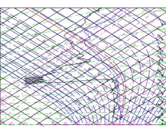
Fig. 1.Sounding from Bauru, 24 February 2004 at 20:15 UTC.

droplets, rain, ice (small ice crystals), snow (low density ice aggregates) and graupel (heavily rimed ice particles), as well as their fall speeds. In order to do this, it assumes that the size spectrum of each hydrometeor is a gamma-type func-tion with coefficients adjustable for each type. The model is single moment for vapour, liquid and rain; i.e., it only has variables for their mass mixing ratios. It is double moment for ice, snow and graupel, in that it can predict both their mixing ratios and number concentrations. The ice scheme is based on Lin et al. (1983), Rutledge and Hobbs (1984), Fer-rier (1994) and FerFer-rier et al. (1995), with refinements from Flatau (1989), Swann (1996) and Swann (1998). The model allows supersaturation of the vapour field with respect to ice with ice being heterogeneously nucleated as a function of this, as based on the Meyers et al. (1992) scheme. Vapour deposition onto ice is based on the supersaturation, the mass and number of the ice field and the assumed shape of the size distributions.

2.2 Meteorology and model initialisation

The simulations shown here were based on a case study day of the 2004 HIBISCUS project, which took place in Bauru, Brazil, located at 22.3◦S, 49.03◦W. The day cho-sen was 24 February, when a sounding (Fig. 1) was made at 20:15 UTC, which is 17:15 LT (local time). It shows a pronounced dry layer centred at∼8.5 km with the cold point and WMO tropopause occurring at∼15.9 km (112 mb – see the end of this section for a discussion on the TTL location). The CAPE (Convective Available Potential Energy) of the sounding was a moderate 1095 J kg−1and the presence of an inversion above the boundary layer resulted in CIN (Convec-tive Inhibition) of∼111 J kg−1.

(4)

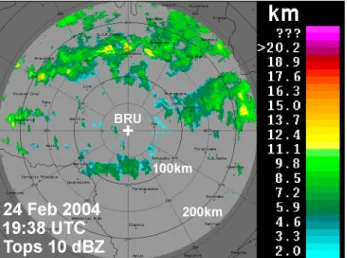
Fig. 2. Echo tops (reflectivity threshold 10 dBZ) observed by the S-band radar in Bauru at 19:38 UTC (=local time+3).

and 12:00 UTC as well as vertical profiles derived at 3-hourly intervals from the Meso-Eta operational mesoscale model (Black, 1994) as run by CPTEC (Centre for Weather Fore-cast and Climatic Studies) for the South American conti-nent, showed CAPE values of between 1144 and 2389 J kg−1 throughout the day, signalling the potential for the devel-opment of severe storms. Cloud tops observed by IPMet’s radars (S-band type at 2.8 Ghz) were mostly<14 km, but a few cells penetrated through the tropopause (tops >18 km at times) during the late afternoon (Fig. 2). Cloud top es-timations from the radar are based on the 10 dBZ echo top for which the errors should be within 1 km for 20 km high clouds at the edge of the radar range and considerably less for clouds that are lower or closer to the radar. Further de-scription of the storms that occurred on this day can be found in Pommereau et al. (2007).

At the time of the radiosonde launch (20:15 UTC), the convective area was ≥100 km north-west to north-east of the radar, with echo tops mostly<10 km, but isolated cells reached up to 15 km. The rain area south of Bauru was already in the dissipation stage. The convection continued throughout the night. Since the closest radiosonde available, viz. Bauru at 20:15 UTC, was released after the initiation of convective events, it is likely that there may be some discrep-ancies between these measurements and the environment that the storms actually formed in, especially in the lower layers, which are subject to heating and moistening, as well as low-level convergence processes.

The latter is known to be occurring in the region as a re-sult of the semi-stationary South Atlantic Convergence Zone (SACZ). This can be identified from satellite images as a cloud band with orientation NW/SE, which commonly ex-tends from the southern region of Amazˆonia into the central region of the South Atlantic (Kousky, 1988), with a typi-cal persistence of≥4 days. It forms along the upper-level

Fig. 3. TITAN-generated image (MDV format) of the storm com-plex on 24 February 2004 at 22:30 UTC. The ellipses demarcate centroids of 20 dBZ reflectivity threshold with a minimum volume of 16 km3.

subtropical jet and to the east of a semi-stationary trough over south-eastern South America, approximately along the Brazilian and Uruguayan coasts at 500 hPa. It is charac-terized by low-level humidity convergence zones, a strong gradient of the equivalent potential temperature in the mid-dle troposphere and an anticyclonic circulation at high levels (200 hPa). Being located at the edge of humid tropical air masses, in regions of strong humidity gradients at low levels, it results in the generation of strong and extensive convective instability. The occurrences of SACZ play an important role in the transfer of latent heat, momentum and humidity from the tropics to the mid-latitudes and are responsible for the most humid periods and heavy summer rainfalls in the State of S˜ao Paulo.

Detailed analysis of radar-derived parameters, using IP-Met’s newly implemented software package TITAN (Thun-derstorm Identification, Tracking, Analysis and Nowcasting; Dixon and Wiener, 1993) with a 20 dBZ reflectivity threshold and a volume of≥16 km3 for the identification of the cen-troid, confirmed the existence of a large multicellular storm complex, lasting for 14.6 h, with a maximum precipitation area of 14 049 km2_{. Figure 3 depicts this complex in}

TI-TAN MDV format (Meteorological Data Volume; Dixon and Wiener, 1993), shortly before reaching Bauru. The large el-lipsis demarcates the envelope of the 20 dBZ centroid, which was tracked to calculate the storm parameters. The Verti-cally Integrated Liquid water content (VIL), another indica-tor of severity, exceeded 7 kg m−2(currently used at IPMet to trigger alerts; (Gomes and Held, 2004) on 11 occasions be-tween 18:57 and 24:07 UTC, with a maximum of 8.3 kg m−2 at 23:37 UTC.

(5)

simulate some extreme cases of convection, it was decided to initiate convection by producing a warm and moist bub-ble in order to artificially increase the CAPE of the environ-ment and to help represent the influx of moist, tropical air as caused by the SACZ. Warm bubbles have been used to ini-tiate deep convection in several CRM studies in the past. In Wang (2003) a 20 km×4 km warm bubble of maximum per-turbation 3.5 K was imposed, which was made moister than its surroundings since the relative humidity was kept con-stant as its temperature increased. In this study the bubble was applied gradually using a heating and moistening rate in the lower 2.5 km of the model domain over a width of 14 km, with the rate decreasing according to a cos2relationship with radial distance from the centre. They were applied for twenty minutes, beginning 5 min after the simulation start and the simulations were performed up to a time of 3 h 35 min. Runs with different heating rates, but with the same rate of mois-ture input, were performed in order to simulate convection with a variety of different strengths. These runs are labelled “3D-med” and “3D-weak” to indicate cells of medium and weaker intensity, with the original case labelled as “3-D”.

One 2-D case was simulated (labelled “2-D”) in which the model domain was 2000 km wide with a 2 km hori-zontal resolution. Such a large domain was required be-cause of interactions of gravity waves emanating from both sides of the cloud due to the periodic boundary conditions of the model, which interfered with the air from the over-shoot. This is much less of an issue in 3-D since the grav-ity waves produced are somewhat smaller in velocgrav-ity mag-nitude than in 2-D. Therefore, in this case the domain is 300×300 km in the “3-D” case and, for computational rea-sons, only 150×150 km in the “3D-med” and “3D-weak” sensitivity tests, with the same resolution. The vertical grid in all cases is 30.4 km deep with the damping layer applied over the upper 7.6 km of the domain. The vertical resolution was 75 m in the boundary layer and 125 m throughout the rest of the domain. Such high vertical resolution is likely to be necessary to properly resolve processes occurring in the TTL, such as the effect of gravity waves on the temperature structure (e.g. Kuang and Bretherton, 2004), and therefore likely on mixing processes too.

It has been demonstrated in previous CRM studies (e.g. Redelsperger et al., 2000), that the use of 2 km horizontal res-olution is fine enough to simulate deep convection reasonably well. But, resolution can have a significant effect on convec-tive mixing processes (e.g. Petch et al., 2002) and therefore may affect the turbulent mixing of overshoot air with the sur-roundings as well as the entrainment of environmental air into the rising air parcel in the boundary layer as observed in Carpenter et al. (1998). The latter would be likely to lead to clouds that are too vigorous due to a lack of dilution by envi-ronmental air from higher levels. These processes would re-quire a resolution finer than 2 km to simulate explicitly (e.g. Lane et al., 2003, and Carpenter et al., 1998, use a horizontal grid spacing of 50 m), although a sub-grid mixing

parame-terisation is included in the model, which may represent this reasonably well. Also, the large ratio of horizontal to vertical grid size may have an unknown effect on the vertical mix-ing and might therefore affect the mixmix-ing of overshoot air in the TTL. In addition, Lane and Knievel (2005) suggest that model resolution affects the spectra of gravity waves formed by CRM models, which can affect whether waves break or not and hence whether mixing due to this process occurs. Further simulations to explore any potential sensitivities to resolution would be desirable, but were too computationally expensive for the current study.

Information on the various runs is displayed in Table 1. The “3D high CCN” case refers to a microphysical sensitiv-ity test case that uses the same heating rates for cloud ini-tiation as the “3-D” case and is described in Sect. 3.4. As the heating rate is decreased, the maximum vertical veloc-ity, which is 50 m s−1_{in the most vigorous case, reduces to}

only 39.3 and 28.4 m s−1_{, respectively, as the clouds became}

less intense. 50 m s−1represents a very high updraught, but one that is within the range of those inferred from obser-vations of tropical deep convection in other tropical regions (e.g. Simpson et al., 1993). The 10 dBZ echotop also reduces in height with cloud intensity from a maximum of 18.2 km to a minimum of 16.4 km in the “3D-weak” case. Interestingly, the 40 dBZ echotop is higher in the “3D-med” case than in the more intense cloud. However, examination of the time-series of maximum echotop heights (not shown) reveals that heights above 14 km were attained only very briefly in the weaker case (one data point in the timeseries where points were calculated every 5 min), whereas 14 km was reached by the 40 dBZ contour for considerably longer in the “3-D” sim-ulation (for three data points in the timeseries).

(6)

Table 1.Information on the different simulations. Columns are the maximum updraught; maximum radar reflectivity; the maximum height of the 10, 35 and 40 dBZ echo tops; the maximum temperature and vapour perturbations in the lower 2.5 km of the domain; and the mean CAPE over the heating area after 5 min of heating.

Run Max updraught (m/s)

Max dBZ Max height of echotop (km): Max temp perturbation (K)

Max vapour mixing ratio perturbation (g kg−1)

Mean CAPE over heating area (J kg−1) 10 dBZ 35 dBZ 40 dBZ

3-D 50 54.7 18.2 17.5 15.1 7.2 2.2 2687

2-D 21.2 53.5 17 13.2 9.7 8.9 2.5 3064

3-D-med 39.3 56 17.4 16.5 15.6 4.1 3.2 2480 3-D-weak 28.4 55.2 16.4 15.3 11.7 3.3 4.2 2449 3-D high CCN 46.3 54.5 18.2 15.9 13.4 7.2 2.2 2687

0 5 10 15 20

12 14 16 18 20

Mixing Ratio (ppmv)

Height

(

k

m

)

24th Feb vapour and ice saturation mixing ratios

Original Sounding 20:15-22:08 UTC Ice Saturation

LEM water vapour

Fig. 4. Water vapour and ice saturation mixing ratio measurements from the 24 February sounding and the idealised vapour profile in-put into the LEM Cloud Resolving Model.

upper range of those predicted by the Meso-Eta mesoscale model.

The main purpose of these simulations is to study the ef-fect of deep convection on the TTL water content. Thefore, in order to avoid the issue of determining whether re-ductions in total water were due to the ice deposition de-hydration effect, or simply due to reversible advection from drier heights, the simulations were initialised with a constant vapour mixing ratio of 5 ppmv around the TTL region, be-tween the heights of 15.77 and 18.93 km, as shown in Fig. 4. This means that any reductions in the total water in this re-gion must have been due to the ice deposition dehydration effect and not reversible transport of the initial vapour field. The value of 5 ppmv corresponds to the approximate vapour mixing ratio in the sounding at the lower and upper boundary of this region and is in line with other measurements of the

TTL water vapour concentrations made at 22:00 UTC at the same location using the micro-SDLA instrument on board another balloon (Durry et al., 2006). This employs the diode laser absorption spectroscopy technique and hence is likely to be more accurate than standard radiosonde measurements, which used the Vaisala RS 80 package.

There are several different ways to define the TTL region, which is generally thought of as a transition zone containing air with both tropospheric and stratospheric properties. The main concern here is how convection affects the water vapour content of air that will enter the stratosphere at some point in the future and hence a useful definition for the TTL base is that of the net zero radiative level (Zrad)as in Sherwood and

Dessler (2000). Based on several different radiation models, Gettelman et al. (2004) foundZrad to be located at a mean

height of 15 km in the tropics with differences due to time and space variations leading to a±500 m change, and inter-model variations giving changes of±400 m. Whether this applies to the region of concern here, though, is unknown.

Since the main temperature inversion of the environment is located at∼15.9 km (Fig. 4) and significant changes in the vertical gradient of the water vapour mixing ratio are appar-ent here, this height is likely to generally serve as an efficiappar-ent mixing barrier to weaker vertical motions and hence if con-vection affects air above this height then it will be very likely to have a stratospheric effect. Therefore, this will be termed the tropopause in future discussions here. According to the radar echo top heights, convection was observed to penetrate the tropopause and so the top of the TTL might be considered to be somewhat higher than 15.9 km, following the conven-tion of Sherwood and Dessler (2000).

2.3 Radar observations

(7)

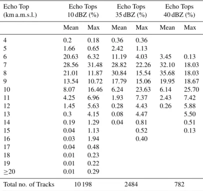
Table 2.Frequencies of echo tops in the height ranges indicated for cell tracks within the 240 km radius range of the IPMet radar in Bauru during the period from 21 January to 11 March 2004. Mean and max labels refer to the frequencies of the mean and maximum echo top of each track during the lifetime of the cell and 10, 35 and 40 dBZ refer to the tops of radar reflectivity contours of these values. Only cells with a volume larger than 50 km3, based on the 10, 35 and 40 dBZ contours, are included in the statistics.

Echo Top Echo Tops Echo Tops Echo Tops (km a.m.s.l.) 10 dBZ (%) 35 dBZ (%) 40 dBZ (%) Mean Max Mean Max Mean Max 4 0.2 0.18 0.36 0.36

5 1.66 0.65 2.42 1.13

6 20.63 6.32 11.19 4.03 3.45 0.13 7 28.56 31.48 28.82 22.26 32.10 18.03 8 21.01 11.87 30.84 15.54 35.68 18.03 9 13.54 10.72 17.79 15.06 19.95 18.67 10 8.07 16.46 6.24 23.63 6.14 25.70 11 4.25 6.96 1.93 7.37 2.43 7.42 12 1.45 5.63 0.28 4.43 0.26 5.88 13 0.3 4.15 0.08 4.47 5.50 14 0.19 1.29 0.04 0.81 0.51

15 0.04 1.13 0.52 0.13

16 0.03 1.94 0.40 17 0.04 0.48

18 0.01 0.23 19 0.01 0.22

≥20 0.01 0.29

Total no. of Tracks 10 198 2484 782

the Bauru area, albeit fairly infrequently. Table 2 shows the percentages of the mean and maximum radar echo tops for the 10, 35 and 40 dBZ reflectivity contours in certain height ranges, for cells where these contours contained storm vol-umes of≥50 km3. They were derived using the TITAN Soft-ware and are based on radar “tracks”, which is the term given to describe the following of a convective cell for its lifetime (including cell splits and mergers) by the software. A total of 10 198, 2484 and 782 cells were identified, using the 10, 35 and 40 dBZ threshold, respectively.

The data shows that the 40 dBZ echo top of one cell (0.13% of the 782 tracks) reached an absolute maximum height of 15–16 km, with 0.64% (5 cells) exceeding 14 km during the 51 day observation period. In addition, the 35 dBZ contour in the “3-D” case reached higher than any of the ob-served events during the campaign (Table 1) and its maxi-mum height in the “3D-med” case (16.5 km) was consistent with only 10 observed events over the campaign. Therefore, based on these higher reflectivities, events as severe as those simulated in the “3-D” and “3D-med” case may represent the upper limit of the convective effect of cells in this area on the TTL region during the experimental period. However, the season in which the campaign took place was less active than previously observed seasons as based on lightning (Nac-carato et al., 2004) and other observations (Pommereau et al.,

2007). Thus, clouds such as those modelled may have been more common in other years.

On the other hand, the maximum height reached by the 10 dBZ contour in the “3-D” case (18.2 km) is consistent with 75 of the observed cells over the campaign. This sug-gests that the model may be predicting too many particles of high mass in the upper troposphere, but that the overall heights reached by the clouds are consistent with reality. In addition, factors such as the beam width divergence (beam width of radar = 2◦)and the possibility of radar scans miss-ing the peak development of clouds due to the time taken to complete a sweep (∼7.5 min), may result in the statistics not representing the higher altitude, high reflectivity contours as consistently as the output from the model.

(8)

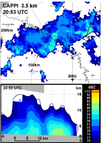
Fig. 5.CAPPI (Constant Altitude PPI at 3.5 km a.m.s.l.) of the mul-ticelluar storm on 24 February 2004 at 20:53 UTC (top), indicating the base line of the cross-section shown on the bottom (gaps due to elevation stepping have been complemented by dotted lines for 10 and 20 dBZ).

3 Model results

3.1 3-D/2-D comparisons

Ideally, it would be possible to be able to simulate the ef-fects of overshooting clouds on the TTL using 2-D models only, since the computational demand of 3-D simulations is huge in comparison. 2-D models have been shown to be able to reasonably simulate some convective systems (e.g. Redelsperger et al., 2000) but have not previously been com-pared with 3-D models in studies concerning the TTL. It is possible that aspects such as the mixing of the overshoot air with the TTL air and gravity wave production may be wrongly represented by 2-D simulations. The latter may have an effect on mixing processes through the breaking of the gravity waves near the TTL (e.g. Lane et al., 2003; Wang, 2003). The degree of mixing is important since it can in-crease the temperature of the overshoot air and hence may help to determine the final settling height of the detrained air as it sinks under its negative buoyancy. In addition, clouds overshooting into the TTL are likely to carry large amounts

of ice with them and thus any mixing of this ice with the TTL air is liable to cause a potentially large moistening effect. In this section, results from a 3-D simulation are presented and compared to those from a similar 2-D case.

3.1.1 General description of cloud features

In response to the heating in the lower layers of the domain a convective thermal was generated that reached just below 18 km by 00:35.

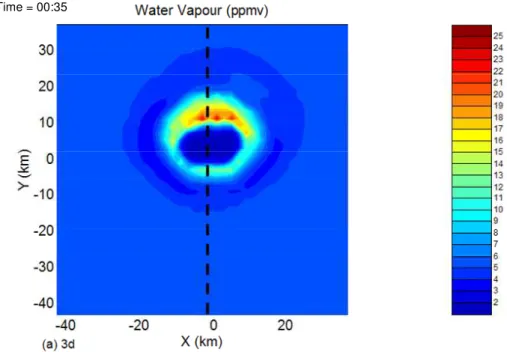
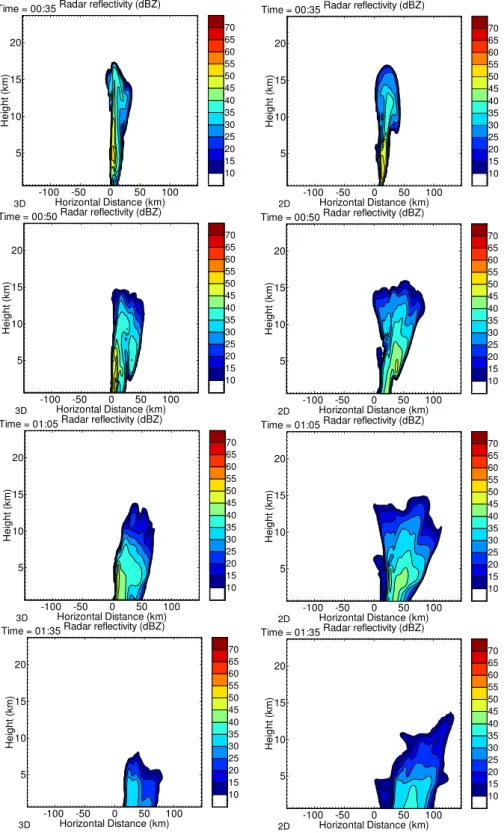
Figure 6 is a horizontal cross-section of water vapour mix-ing ratio through the simulated 3-D cloud at 16.5 km and 00:35, to give an idea of the location of the overshoot in the model domain. This height is already above the tropopause of the simulation environment and hence is likely to be within the TTL region. The effects on the water vapour are dis-cussed shortly, but first of all the simulated radar reflectivi-ties of a cross-section (dotted line in Fig. 6) through the cloud are examined and compared to the 2-D case in order to ex-amine the general cloud features throughout the troposphere (Fig. 7).

The radar reflectivities, calculated every 5 min, show that the initial stages of the overshoot were more vigorous and reached higher altitudes in the 3-D case compared to the 2-D one, despite the same heating and moistening rates being ap-plied. For example, the 35 dBZ contour has reached up to just under 17 km by 00:35 in the 3-D case, whereas it was only at∼13 km in the 2-D case. In addition, the 40 dBZ reflec-tivity contour reached 15.1 km in one of the samples of the simulated cloud reflectivity in the 3-D case, which were cal-culated every 5 min. By contrast, the 40 dBZ contour of the 2-D case reached a maximum height of only 9.7 km. This in-dicates increased flux of larger ice hydrometeors in the 3-D case compared to that of the 2-D case. After this time, the 2-D and 3-D cases show qualitatively similar clouds in terms of shapes and sizes, although in general the 2-D cloud was a little wider than that in the 3-D simulation. This is especially apparent for the last time shown, where the 2-D cloud also extended up to higher altitudes. The width of the clouds dur-ing the growth and decay phases was generally similar to the sizes of clouds observed by the IPMet radar suggesting that the warm and moist bubble used was producing a cloud of a realistic size.

(9)

Time = 00:35 Time = 00:35

Fig. 6.Horizontal cross-sections at a height of 16.5 km of the water vapour mixing ratio at 35 min of simulation time for the 3-D case. The dotted line represents the location of vertical cross-section shown in the following figures.

to potentially have had an impact on the low water content of the TTL. Radar reflectivities of up to 54–55 dBZ were sim-ulated in the interior of the cloud, which matched the maxi-mum observed at similar heights by the IPMet radar on this day (54 dBZ).

A comparison of the simulated storm structures with radar observations from this day yielded a reasonable agreement, as demonstrated in the vertical cross-section in Fig. 5. The horizontal and vertical extents of the cell, selected from the storm complex, are approximately the same magnitude as in the simulation, even including the distribution of the higher radar reflectivities (cell core).

The maximum updraught speeds of the clouds show sig-nificant variation between the 2-D and 3-D cases with the absolute maximum being 21 m s−1at an altitude of 6.7 km for the former and 50 m s−1at 12.5 km in the latter case. The increased vigour of the 3-D case relative to the 2-D one sug-gests that some of the differences in the behaviour of the two overshooting clouds in the TTL that will be shown here, may be due to the increased mass flux and ice transport of the 3-D case. Further tests with less vigorous 3-D clouds are there-fore examined later in order to determine whether or not this is the case.

3.1.2 The effect on TTL water content during the simula-tion

Figure 6 demonstrates that in the 3-D case the water vapour content at 16.5 km has been depleted significantly below the initial environmental value through cold temperature ice

de-position. As well as the depleted vapour air formed in the core of the overshoot, though, considerable vapour increases have also occurred in the surrounding air, with values as high as 25 ppmv being reached. This time corresponds to that when the minimum vapour mixing ratio was achieved in the 3-D case (see Fig. 10).

The vertical slices (Fig. 8) show some similarities between the 3-D and 2-D cases with a similar size of overshoot dis-turbance and similar minimum values produced in both cases (0.57 ppmv in 3-D and 0.62 ppmv in 2-D). The area covered by the low vapour air is, however, significantly smaller in the 3-D case and there is a large area of high vapour con-tent in the 3-D case that covers approximately half the area of the dehydrated air seen in the 2-D simulation. In addi-tion, the boundary between the high vapour air below and the depleted vapour above is much more irregular in the 3-D case, indicating that more mixing due to small scale motions is occurring. Considerable amounts of ice were present in both cases (see contours in Fig. 8) in the same area as the overshoot air, allowing the possibility of significant moisten-ing through sublimation of this ice and makmoisten-ing this a likely explanation for the high vapour air that was seen in the 3-D case.

(10)

10 15 20 25 30 35 40 45 50 55 60 65 70

-100 -50 0 50 100

5 10 15 20

Horizontal Distance (km)

Hei g ht ( k m )

Radar reflectivity (dBZ) Time = 00:35

3D 10 15 20 25 30 35 40 45 50 55 60 65 70

-100 -50 0 50 100

5 10 15 20

H ei ght ( k m )

2D 10 15 20 25 30 35 40 45 50 55 60 65 70

-100 -50 0 50 100

5 10 15 20

He ig ht ( k m)

3D 10 15 20 25 30 35 40 45 50 55 60 65 70

-100 -50 0 50 100

5 10 15 20

H ei ght ( k m )

2D 10 15 20 25 30 35 40 45 50 55 60 65 70

-100 -50 0 50 100

5 10 15 20

H ei ght ( k m )

3D 10 15 20 25 30 35 40 45 50 55 60 65 70

-100 -50 0 50 100

5 10 15 20

H ei ght ( k m )

2D 10 15 20 25 30 35 40 45 50 55 60 65 70

-100 -50 0 50 100

5 10 15 20

H ei ght ( k m )

3D 10 15 20 25 30 35 40 45 50 55 60 65 70

-100 -50 0 50 100

5 10 15 20

H ei ght ( k m )

2D 10 15 20 25 30 35 40 45 50 55 60 65 70

-100 -50 0 50 100

5 10 15 20

Hei g ht ( k m )

3D 10 15 20 25 30 35 40 45 50 55 60 65 70

-100 -50 0 50 100

5 10 15 20

H ei ght ( k m )

2D 10 15 20 25 30 35 40 45 50 55 60 65 70

-100 -50 0 50 100

5 10 15 20

He ig ht ( k m)

3D 10 15 20 25 30 35 40 45 50 55 60 65 70

-100 -50 0 50 100

5 10 15 20

H ei ght ( k m )

2D 10 15 20 25 30 35 40 45 50 55 60 65 70

-100 -50 0 50 100

5 10 15 20

H ei ght ( k m )

3D 10 15 20 25 30 35 40 45 50 55 60 65 70

-100 -50 0 50 100

5 10 15 20

H ei ght ( k m )

2D 10 15 20 25 30 35 40 45 50 55 60 65 70

-100 -50 0 50 100

5 10 15 20

H ei ght ( k m )

3D 10 15 20 25 30 35 40 45 50 55 60 65 70

-100 -50 0 50 100

5 10 15 20

H ei ght ( k m )

2D

(11)

-50

0

50

14

15

16

17

18 H

e

ig

h

t (km)

Vapour Mixing Ratio (ppmv)

5

1 0

1

0

1

5

1

5

2

0

(a) 3D

Time = 00:35 UTC

0.57

1.6

2.6

3.6

4.6

5.6

6.6

7.6

8.6

9.6

11

12

13

14

15

16

17

18

19

20

21

22

23

24

25 -50

0

50

14

15

16

17

18 Horizontal Distance (km)

Height

(

k

m

)

5

10

1

0

1 5

(b) 2D

Fig. 8.Water vapour mixing ratio fields after 35 min of simulation time:(a)Cross section through the line indicated in Fig. 6 of 3-D simulation;(b)2-D case. The white contours indicate the total ice mixing ratio (ice+snow+graupel) in ppmv×103.

sublimation and was responsible for the large water vapour mixing ratio values produced. In the 2-D case such intrusion of high potential temperature air has not occurred, suggest-ing that the use of 3-D has a large impact on the mixsuggest-ing of the overshoot air with its surroundings.

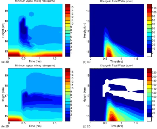
Figure 10 shows the minimum water vapour mixing ra-tio achieved over each height and at each time (5 min sam-ples) in the 3-D and 2-D cases. It demonstrates that in the 3-D case lower vapour values are reached (a minimum of 0.2 ppmv compared to 0.6 ppmv in 2-D) on account of the 3-D case producing a more vigorous updraught, which leads to lower temperatures. These low values also occur at higher altitudes (height of minimum is 17.9 km in 3-D and 17 km in 2-D), again symptomatic of the higher updraughts in the 3-D case. However, the low vapour values quickly disappear in the 3-D case so that after∼50 min the minimum vapour value is 4.97 ppmv, which is very close to the initial mini-mum vapour mixing ratio of the TTL (5 ppmv). In the 2-D simulation, air that is significantly vapour depleted remains

-50

0

50

14

15

16

17

18 H

e

ig

h

t (km)

Potential Temperature (K)

5 5

10

1₀

1

5

1

5

2₀

(a) 3D

Time = 00:35 UTC

349

352

355

358

361

364

367

370

373

376

379

382

385

388

391

394

397

400

403

406

409

412

415

418

421

424

427

430

433 -50

0

50

14

15

16

17

18 Horizontal Distance (km)

Height

(

k

m

)

5

1 0 1₀

15

(b) 2D

Fig. 9.As for Fig. 8, but for the potential temperature.

until the end of the simulation time, with the minimum be-ing 3.3 ppmv at that time. The persistence of the low vapour air allows time for the separation of the ice formed, to leave behind low total water air. This lack of ice is important in determining whether permanent dehydration is likely to oc-cur since ice sublimation cannot then replenish the vapour of the air, which may otherwise happen as the cold air sinks and warms under its negative buoyancy, or through mixing with warmer surrounding air, as observed in the 3-D case. The lo-cation of the ice as it sinks downwards is demonstrated by the total water time-height plot in Fig. 10 where the reduction in total water in 2-D can also be seen.

(12)

0 20 40 60 80 100 120 140 160 180 200 220

0 0.5 1 1.5

15 16 17 18 19 Time (hrs) Hei g h t ( k m )

Change in Total Water (ppmv)

(b) 2D 0 10 20 30 40 50 60 70 80 90 100 110

0 0.5 1 1.5

15 16 17 18 19 Time (hrs) H e ight ( k m )

(a) 3D 1 2 3 4 5 6 7 8 9 10 11 12 13 14 15

0 0.5 1 1.5

Minimum vapour mixing ratio (ppmv)

(b) 2D 1 2 3 4 5 6 7 8 9 10 11 12 13 14 15

0 0.5 1 1.5

(a) 3D 0 20 40 60 80 100 120 140 160 180 200 220

0 0.5 1 1.5

(b) 2D 0 10 20 30 40 50 60 70 80 90 100 110

0 0.5 1 1.5

15 16 17 18 19 Time (hrs) H e ight ( k m )

(a) 3D 1 2 3 4 5 6 7 8 9 10 11 12 13 14 15

0 0.5 1 1.5

(b) 2D 1 2 3 4 5 6 7 8 9 10 11 12 13 14 15

0 0.5 1 1.5

(a) 3D

Fig. 10.Time-height plot of the minimum water vapour mixing ratio (left) and the domain mean total water (right) for;(a)The 3-D case;(b)

the 2-D case.

by gravity waves that emanated from the cloud sides after the overshoot penetrated the stable layer of the tropopause. Similar waves appear on the other side, to the right of the area shown in Fig. 11 (not visible on the plot). Such waves did occur in the 3-D case, but with smaller displacements as demonstrated by Figs. 8 and 9.

The differences in the velocity magnitudes of the waves in the TTL between the 2-D and 3-D cases can be demon-strated by the maximum updraught velocities (not shown). Despite the initial overshoot updraught in the 3-D case be-ing larger and extendbe-ing to higher altitudes, the updraughts quickly dissipate to leave very little wave motion, whereas in the 2-D case the upwards velocities due to wave motions persist throughout the simulation.

These gravity waves were responsible for some vapour re-moval in the 2-D case, as indicated by the dry air formed above the crest of the wave in Fig. 11 and hence, the larger wave magnitudes seen in 2-D may be somewhat responsible for the perseverance of the low vapour air seen in this case, but not in 3-D. The bulk of the dehydrated air, though, was left over from the initial overshoot and hence the differences in the mixing occurring during this event were likely to have been the main cause of the 3-D/2-D differences. The large differences in gravity wave behaviour and the differences in mixing observed suggest that the 2-D version of the present model is not well suited to simulating overshoot dynamics.

3.1.3 Overall effects at the simulation end

By the end of the simulation, the once negatively buoyant air detrained by the overshoot has almost reached its level of neutral buoyancy again in both the 2-D and 3-D cases, as judged from potential temperature perturbations (not shown). The 2-D case exhibited the largest perturbations relative to the initial state, but those of the air detrained from the over-shoot had a maximum negative perturbation of∼5 K, which was typical of the potential temperature from the region only 250 m below, indicating that this air would only go on to sink by this amount, or less. The 3-D case showed even smaller perturbations throughout the TTL. This suggests that the sit-uation at the simulation end is likely to be representative of the permanent effect of the convection in the TTL, barring the longer term effects of processes not included in the model, such as radiative effects and the Brewer Dobson circulation.

(13)

-100 -50

0

50

100

14

15

16

17

18 H

e

ig

h

t (km)

Vapour Mixing Ratio (ppmv)

(a) 3D

Time = 01:35 UTC

2

3

4

5

6

7

8

9

10

11

12

13

14

15

16

17

18

19

20

21

22

23

24

25 -100 -50

0

50

100

14

15

16

17

18 Horizontal Distance (km)

Height

(

k

m

)

(b) 2D

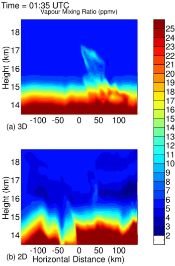
Fig. 11.As in Fig. 8, but for the time of 01:35.

depleted in total water with the overall mean total water be-ing reduced above 15.84 km. Below this height, however, the 2-D simulation causes a mean moistening of a magnitude that appears larger than in the 3-D case.

However, care must be taken in the comparison of the 2-D and 3-D means since the 2-D mean is taken over only one 300 km long 2-D slice, whereas in the 3-D case, the mean over 150 slices of width 2 km is taken, to give the average across the whole 300×300 km domain. Since the horizon-tal cross section of the cloud outflow is roughly circular, the number of points in these slices that have been affected by the overshoot will reduce for slices further from the centre of the outflow. Therefore, the deviations of the 3-D mean from the background value will be “diluted” since more air with the background value is included in the summation. It can be shown that the mean changes along slices of the 3-D domain can be more significant than the changes observed in the 2-D case.

An attempt is made here to use the 3-D results to estimate how representative the mean changes across 2-D slices of the 3-D domain are of the full 3-D mean total water change at

-1 0 1 2 3 4 5

15 15.5 16 16.5 17

Change in mixing ratio (ppmv)

Height

(

k

m

)

2D tot 2D vap 2D tot scaled 3D tot 3D vap

Fig. 12. The change in mean vapour and total water mixing ratios for the 2-D and 3-D cases at the simulation end (time=3 h 35 min). In the 2-D case the mean is taken over the central 300 km of the overshoot area. “2-D tot scaled” refers to the mean 2-D change multiplied by a scaling factor of 0.22 to represent the likely overall 3-D effect of such a 2-D slice if it represented just one slice out of a 300 km×300 km domain.

each height. This is done by assuming that the 2-D slice, from the 3-D simulation, showing the highest mean change at each height is representative of the 2-D simulation. The ratio of the mean change across this slice to the full mean change across the whole 300×300 km area at that height then gives some indication of how much a 2-D change should be scaled by in order to better represent the change over a 3-D surface. This ratio of the mean change over the full 3-D area to that of the 2-D slice exhibiting the largest change, has an average value of 0.22 between 15 and 17 km based on the 3-D total water field at the end of the simulation. The 2-D mean total water changes shown in Fig. 12 are multiplied by this value for a fairer comparison to the 3-D results (“2-D tot scaled” line). After scaling, the total water increases in the lower TTL become somewhat lower than in 3-D, indicating the importance of the consideration of the 2-D results in a 3-D context.

(14)

10 15 20 25 30 35 40 45 50 55 60 65 70

-20 0 20

5 10 15 20

He ig h t ( k m )

(a) 3D 10 15 20 25 30 35 40 45 50 55 60 65 70

-20 0 20

5 10 15 20

He ig h t ( k m )

(b) 3D-med 10 15 20 25 30 35 40 45 50 55 60 65 70

-20 0 20

5 10 15 20

He ig h t ( k m )

(c) 3D-weak 10 15 20 25 30 35 40 45 50 55 60 65 70

-20 0 20

5 10 15 20

He ig h t ( k m )

(a) 3D 10 15 20 25 30 35 40 45 50 55 60 65 70

-20 0 20

5 10 15 20

He ig h t ( k m )

(b) 3D-med 10 15 20 25 30 35 40 45 50 55 60 65 70

-20 0 20

5 10 15 20

He ig h t ( k m )

(c) 3D-weak

Fig. 13.Cross sections of the simulated radar reflectivity of the 3-D cases of various strengths taken though the slice inidicated in Fig. 6.

the tropopause (15.9 km), suggesting that direct moistening of the stratosphere has occurred here, although the increases at these high altitudes are much lower than those below the tropopause.

3.2 Weaker 3-D cases

It is possible that the extra mixing in the 3-D case that re-sulted in moistening of the TTL, rather than the dehydration seen in 2-D, may have been due to the increased vigour of the 3-D case relative to the 2-D one and hence, that a weaker storm in 3-D might also produce dehydration. In order to test this, less severe 3-D cases are examined here to look for any occurrence of dehydration. Table 1 reveals that the weaker cases generally had significantly lower maximum updraughts and maximum heights of the various simulated echo tops, but that the weakest case still had a 10 dBZ echotop at 16.4 km and thus penetrated the tropopause.

Figure 13 shows cross sections of the simulated radar re-flectivity for the different strength cases, taken at the times when the 10 dBZ echo top reached its highest altitude in each separate case. These times were all different since the clouds took longer to develop when lower heating rates were ap-plied. It shows that as the clouds become less intense, the radar echoes become narrower in the upper regions, which is more in agreement with the observed cross section from the case study day (Fig. 5). In addition, the 35 dBZ echo contour is seen to reach successively lower heights, which is also more consistent with the observations. However, in gen-eral all the cases have simulated echoes in the upper regions of the cloud that are higher than those observed on the 24 February, 2004. For example, even in the weakest case, the 35 dBZ echotop reaches around 15 km, whereas in the ob-served cross section it only gets to∼7 km. Radar statistics for the whole campaign show that 23 events are consistent with the maximum height of the 35 dBZ contour reached in the “3-D-weak” case, whereas as only 10 were consistent for the height reached in the “3-D-med” case and none for the “3-D” case. However, the height of the 40 dBZ contour was consistent with 152 cells for the “3-D-weak” case, but only 1 cell for the “3-D-med” and “3-D” cases. The maximum heights of the simulated 10 dBZ contours were in line with more of the observed storms; 322 for the “3-D-weak” and 124 for the “3-D-med” case.

(15)

(16.4 km) and even of that of the strongest case (18.2 km) are considerably lower than that observed for a significant num-ber of the observed cells, suggesting that some of the real clouds reached higher than those simulated, and that it may be inaccuracies in the model microphysics or the treatment used to calculate the radar reflectivites from the model fields that are leading to artificially high simulated radar reflectivi-ties.

Most of the simulated reflectivity in the upper regions can be shown to be due to the graupel hydrometeor since the re-flectivity is much larger for bigger particles. Such particles are likely to fall out quickly from the overshooting cloud and would evaporate more slowly upon mixing with stratospheric air. Therefore, their presence might indicate an underestima-tion of the amount of moistening that would occur in reality, assuming that the total mass of water transported to the upper cloud is accurate. If this is the case, it may be that the overall height reached by the cloud, which is perhaps better captured by the 10 dBZ echotop, is more representative for estimating the number of real events that are likely to have had an effect on the TTL water content that is similar to those simulated. Then, comparisons of the high reflectivity contours may not be useful. On the other hand, increased amounts of graupel could indicate that too much water mass is being transported upwards by the cloud, perhaps due to a lack of removal by precipitation lower down or a lack on entrainment of dry air into the lower regions of the cloud caused by inaccuracies in the model dynamics. Further simulations and comparisons to observations are required to determine which is the case.

Figure 14 shows the mean vapour and total water change at the end of the simulation relative to the simulation start. It shows that, in all cases, moistening is observed and since the weakest cloud here has little effect at the altitudes where the dehydration was observed in 2-D and since the 10 dBZ echotop is lower than that for the 2-D cloud, it suggests that a weaker still cloud would be unlikely to produce dehydra-tion at similar altitudes to that observed in the 2-D cloud. Therefore, it seems likely that it was the 3-D dynamics that allowed extra mixing, rather than the increased severity of the 3-D case. Plots of the minimum vapour mixing ratio, similar to Fig. 10a (not shown), reveal similarly rapid removal of the low vapour air via mixing.

The amount of moistening reduces significantly with the intensity of the cloud, as might be expected, since there will be less upwards mass flux of ice with the lower updraught clouds. Above 16 km, there is very little ice mass remain-ing in any of the cases. Between here and 17 km, the aver-age increases in the vapour mixing ratio are 0.30, 0.092 and 0.013 ppmv in the “3-D”, “3-D-med” and “3-D-weak” cases, respectively. Between 15 and 16 km, the mean increases are, in the same respective cases, 1.0, 0.83 and 0.76 ppmv. In this lower region there is only significant ice remaining in the “3-D” case, which allows the possibility of vapour increases in this case through evaporation of this ice in the future.

-0.5 0 0.5 1 1.5 2 2.5 3 3.5 4 15

15.5 16 16.5 17 17.5 18 18.5

Mixing Ratio (ppmv)

Height

(

k

m

)

3D vap 3D-med vap 3D-weak vap 3D tot 3D-med tot 3D-weak tot

Fig. 14. The change in mean vapour and total water mixing ratios, at the simulation end, for the various 3-D cases. Means are taken over the central 150 km of the domains.

3.3 Assessing the potential global significance of the TTL water effects

In order to put the changes seen in the above cases into con-text in terms of a global stratospheric effect, the mechanism by which the air affected by the clouds is likely to be trans-ported into the stratosphere must be considered. The pro-cess assumed here is similar to that envisaged by Sherwood and Dessler (2001), whereby air is horizontally processed through regions of frequent deep convective activity, which affect the TTL water content. Net lofting of the air above the net zero clear sky radiative lifting level (Zrad)is then

as-sumed to mainly occur outside of the convective regions. A rough estimate of the effect on a parcel of air moving through such a convective area is made by assuming that all convective events behave in the same way as those simulated and that their effect is spread evenly across the area. If there

are dN/dt events per unit area and each changes the total

water mixing ratio of a region of air of areaA=150×150 km2 and thicknessHbydq, then the overall change in total water mixing ratio of the parcel is approximately given by

dQ=AdN

dt dqτ (1)

whereτ is the amount of time spent in the area.τ is approx-imated by the length of the convective area divided by the speed at which the parcel travels through it. A typical hori-zontal wind speed at TTL height is 5 m s−1_{(e.g. Holton and}

Gettelman, 2001) and the size of a region of high convective activity, such as that occurring over South America, might be∼2000 km or more based on the areas of frequent over-shooting clouds identified by satellite observations in Liu and Zipser (2005). This would give aτ value of∼4.6 days.

dN/dt is estimated from the TroCCiBras/HIBISCUS

(16)

Table 3.dQvalues (Eq. 1) for the different runs. These were made based on the observed numbers of cell tracks whose maximum echo top heights were consistent with the simulated maximum echo top (from Table 2), for reflectivity thresholds of 10, 35 and 40 dBZ.dqvalues based on averages of vapour changes only, over both 15–16 km and 16–17 km, are used.

Based on echo tops of:

10 dBZ 35 dBZ 40 dBZ MeandQ(ppmv) over:

Run 15–16 km 16–17 km 15–16 km 16–17 km 15–16 km 16–17 km 3-D 0.85 0.26 0 0 0.012 0.0034 3D-med 1.17 0.13 0.093 0.01 0.0095 0.0011 3D-weak 2.8 0.047 0.2 0.0034 1.3 0.022 3D high CCN 0.98 0.28 0.3 0.085 0.63 0.18

simulated echo top heights for the 10, 35 and 40 dBZ reflec-tivity contours. These numbers were divided by the 51 days over which observations were made and by the area of the IP-Met radar range (circle of radius 240 km) to give an average frequency per unit area. The value ofdqfor a height range was estimated from Fig. 14 using the increases in vapour only. The height ofZrad is critically important in the

cal-culation, since the lower it is, the more moist air from below the tropopause is likely to be lofted into the stratosphere.

One estimate ofdqis made using the height of 15 km for

Zrad(Gettelman et al., 2004) and by averaging over an

arbi-trary height of 1 km. The thickness of the air parcel chosen for this average becomes important when considering how often air, on its way into the stratosphere, would have to pass through a convective region so that a constant supply of air affected by convection entered the stratosphere. With a typical ascent rate of just over 1 km month−1_{(e.g., Holton}

and Gettelman, 2001) all the air parcels in the 1 km region would need to be affected by convection approximately ev-ery month, if thedQvalue estimated here is to apply to the stratospheric entry mixing ratio of air. However, an estima-tion of the frequency that trajectories on the way into the stratosphere sample convective regions is beyond the scope of this study. The moistening estimates given here are in-tended to give a rough idea of the effect on 1 km deep air parcels as they make one traverse through a convective re-gion and not on the overall stratospheric effect.

dq values for the height range 16–17 km are also made since the air here is above the tropopause and therefore moistening at these heights would be almost certain to have a stratospheric effect.dQvalues based on the different height ranges and convective frequencies are presented in Table 3 for the three different 3-D cases. Water vapour, rather than total water, was used since it is possible that the remaining ice will sediment to below 15 km and hence not cause per-manent moistening.

The results suggest that the moistening observed above the tropopause, between 16 and 17 km, is only likely to signifi-cantly affect air on its way into the stratosphere if events, such as those simulated here, occur with a frequency on a

par with those observed to have 10 dBZ echo tops as high as those simulated; i.e., if the height of the 10 dBZ echo top is indicative of the likely moistening potential of a cloud. This is possible since even clouds with 10 dBZ radar reflectivi-ties in the upper regions are still likely to transport amounts of water mass that are large enough to significantly affect the relatively dry TTL and stratosphere. In the case that the 10 dBZ echo tops are representative of a similar moistening to that simulated, and if convection is only likely to affect the stratosphere if it moistens air above 16 km, the result from the vigorous “3-D” case suggests that a 1 km deep layer of air might have its mixing ratio increased by∼0.26 ppmv when travelling though the convective region for 4.6 days. The predicted moistening in the “3-D-med” case is half this value. Both of these suggest a potentially fairly significant moistening of stratospheric air due to convection.

If air above 15 km is lofted into the stratosphere via the Brewer Dobson circulation, then much more moistening is likely. The most moistening is predicted for the “3-D-weak” case, since the heights of the various simulated echo tops were consistent with more of the observed clouds. For this case,dQvalues of up to 2.8 ppmv are predicted when based on 10 dBZ echo top statistics. Such a moistening would be highly significant as it represents a large fraction of the stratospheric water vapour mixing ratio. However, because the simulated 35 dBZ echo top was consistent with a lot fewer of the observed clouds and since the height of Zrad

is uncertain, it is possible that this is an overestimate. In-deed, if the cloud frequency consistent with the simulated 35 dBZ echo top height is used, a more moderate moisten-ing of 0.2 ppmv is predicted for the “3-D-weak” case. For the other cases, very small moistening values of less than 0.012 ppmv are calculated when using either the 35 dBZ con-sistent frequencies or the 40 dBZ concon-sistent ones, reflecting the tendency for those simulations to overestimate the reflec-tivity in the upper regions of the cloud.

(17)

based, hence meaning that the air would have to travel equa-torwards before this was possible. Even if this does occur the air is likely to be below the local cold point and hence will have to ascend through it to reach the stratosphere. This may result in dehydration of the moistened air and may therefore reduce the impact of the convective moistening on the strato-sphere for the air below the Bauru tropopause. However, since air at the cold point can often be sub-saturated there is potential for moisture transported up to below the cold point to play some role in increasing the moisture content of air entering the stratosphere, relative to that which would have crossed the cold point had the convection not occurred.

Overall, the results suggest that the issues of whether air below the tropopause is likely to affect the stratosphere later on and whether clouds with similar 10 dBZ echo tops to those simulated will have a similar stratospheric moistening to that predicted by the simulations, despite generally having lower echo tops for the higher reflectivity contours, will be key in predicting the stratospheric effect of convective clouds based on these and other CRM simulations.

3.4 Microphysical considerations and CCN sensitivity The ice content and size distribution of the ice in the over-shoot are likely to be key to determining the fall speed of the ice and hence at what rate it separates from the low vapour content air. Lower fall speeds will allow more ice evapora-tion upon mixing with the surrounding air and could result in a moistened TTL, whereas higher sedimentation rates may allow the majority of the ice to separate from the vapour-depleted air before mixing can occur and lead to dehydra-tion of the TTL. It will be shown in this secdehydra-tion that the ice mass and number concentrations in the overshooting air of these simulations are largely determined by microphysical processes occurring in the mid-troposphere, which therefore are likely to have an important effect on how an overshooting cloud affects the TTL water content. Increases in the aerosol loading of a cloud are known to affect cloud microphysics significantly through the activation of more CCN into water droplets at cloud base (e.g., Rosenfeld and Woodley, 2000) and hence the results from the previous section might be ex-pected to be sensitive to this. This is explored using the same set up as in the “3-D” simulation described above, except a smaller horizontal domain of 150×150 km is used.

In the CRM used in these studies, CCN variation is sim-ulated through the warm rain process and the homogeneous freezing parameterisations. The model employs the Kessler (1969) warm rain parameterisation with modifications fol-lowing Swann (1996). In this scheme, the increase in rain mixing ratio due to conversion from cloud droplets is pro-portional to the liquid water mixing ratio above a threshold value. No conversion occurs below this threshold mixing ra-tio, which is that of a population ofnLdroplets of

diame-ter 20µm. This number is assumed constant throughout the cloud and is varied to simulate the effect of changes in CCN.

So, references to CCN number here refer to CCN that acti-vate to form droplets. Increasing the value ofnLhas the

ef-fect of increasing the threshold cloud liquid mixing ratio and thus delaying the onset of rain formation by auto-conversion. Increased droplet numbers allow more ice crystals to form when they freeze homogeneously at around –38◦C. The num-ber of ice crystals produced is proportional to the mass of liquid that freezes, but with the number formed per kilogram of air limited below the number of droplets per kilogram of air at cloud base. This is approximately equal to the input CCN number per cubic centimetre, as the air density is close to unity at cloud base. This means that fewer ice crystals per cubic centimetre can form at the low air densities of the up-per troposphere than the input concentration of droplets up-per cubic centimetre.

Although this is an approximation, aircraft observations from Rosenfeld and Woodley (2000) suggest that large ice crystal number concentrations do indeed freeze homoge-neously as a result of large droplet numbers at cloud base. They found that∼200–400 cm−3ice crystals were formed in the homogeneous freezing zone from droplet numbers of up to∼800–1000 cm−3in the lower troposphere. Similar num-bers were also produced using a CRM with explicit micro-physics in Khain and Pokrovsky (2004). At the air density of 0.4 kg m−3at –38◦C, as based on the sounding used in the simulations here, this ice crystal number concentration cor-responds to 500–1000 kg−1, suggesting that the assumption in the high CCN case of ice crystal numbers at the homo-geneous freezing level being limited to the same number of droplets per kilogram of air as at cloud base may be valid.

The default value ofnL, as used in the previous

simula-tions, is 240 cm−3; for this sensitivity test this is increased to 960 cm−3. The activation of droplets of concentration 240 cm−3is a fairly low number, more typical of maritime than continental conditions for the magnitudes of updraught speeds simulated here, whereas concentrations of 960 cm−3

are more associated with a continental environment (e.g., Twomey, 1959).