An Integer Programming Formulation for the Lot
Streaming Problem in a Job Shop Environment
with Setups
Udo Buscher and Liji Shen
Abstract—This paper aims at solving the lot streaming prob-lem in a job shop environment, where setup times are involved. The proposed integer programming formulation sufficiently describes the processing dynamics of individual sublots and en-ables the simultaneous determination of schedules on machines and sublot sizes. Small instances of job shop problems with consistent sublots can thus be optimally solved. Computational results confirm that, by applying the lot streaming strategy, both idling times of machines and completion times of operations are significantly reduced. In view of setups, various types of setups are incorporated in the model. The influence of setup times on the performance of lot streaming is also intensively examined. In addition, the efficiency of the formulation with special constraints is evaluated.
Index Terms—lot streaming; job shop scheduling; integer programming
I. INTRODUCTION
T
HE purpose of this paper is to solve the lot streaming problem in a job shop environment, where setup times are involved. The job shop scheduling problem can be briefly described as follows: A set of jobs and a set of machines are given. Each machine can process at most one job at a time. Each job consists of a sequence of operations, which need to be processed during an uninterrupted time period of a given length on a given machine. A schedule is an allocation of the operations to time intervals on the machines. The objective is to find a schedule of minimum length (makespan). This class of problems is proved to be NP-hard.With respect to lot streaming, a job is actually a lot composed of identical items. In classical job shop scheduling problems a lot is usually indivisible. The entire lot must be completed before being transferred to its successor operation, which leads to low machine utilization and long completion times. Lot streaming techniques, on the other hand, provide the possibility of splitting a lot into multiple smaller sublots, which can be treated individually and immediately trans-ferred to the next stage once they are completed. Different sublots of the same job can thus be simultaneously pro-cessed at different operation stages. As a result of operation overlapping, the production can be considerably accelerated. However, due to the complex interaction between sublots and machines, job shop problems with the application of the lot streaming strategy is difficult to formulate mathematically.
In the last years, a majority of researches focused on solv-ing lot streamsolv-ing problems in a flow shop production system
Manuscript received December 7, 2010; revised January 30, 2011. Udo Buscher is full professor of industrial management at the Dresden University of Technology in Germany. e-mail: [email protected]
Liji Shen is currently a research associate of Professor Buscher at the Dresden University of Technology. e-mail: [email protected]
[1], [9], [10], [4], [5], [2], [7]. The job shop scheduling prob-lem, on the contrary, has received little attention. Dauz`ere-P´er`es and Lasserre [6] introduced an iterative heuristic to solve the lot streaming problem in a job-shop environment. By adopting the modified shifting bottleneck procedure, a good solution can be obtained within a few iterations. For the same problem, Buscher and Shen [3] presented an advanced tabu search algorithm which outperforms the previous heuris-tic. This algorithm is also able to reach the theoretical lower bounds for some hard benchmark instances in scheduling. In [8] a model for the lot streaming problem with setups was established. Aside from the makespan objective, cost-based measurements are integrated as well. Under the assumption that the sublot sizes are given, several examples were tested with the conclusion that equal-sized sublots provide better solutions in general.
The integer programming formulation presented in this paper is based on the study of [8]. Necessary modifications are conducted in the first place. The model is then further developed to increase efficiency. Moreover, instead of em-ploying fixed sublot sizes, test instances are solved with the determination of sublot sizes. According to our observation, optimal solutions are generally obtained with unequal-sized sublots, which obviously contradicts the assertion of [8].
The remainder of the paper is organized as follows: In the next section, an integer programming formulation for solving the lot streaming problem in a job shop production system with setups is developed. Various types of setups are incorporated in the model. Section 3 provides a detailed analysis of computational results. The computational results focusing on various aspects are then presented in detail. Brief conclusions are summarized in Section 4.
II. MODEL FORMULATION
A. Notations
Cmax makespan
n total number of jobs
m total number of machines
s total number of sublots
i, i′ job indices,i, i′= 1, . . . , n
k, k′ machine indices,k, k′ = 1, . . . , m
j, j′ sublot indices,j, j′= 1, . . . , s
H sufficiently large number
Di demand of jobi, i.e. the initial lot size
Mk machinek
Oijk the operation of thejth sublot of job i
tijk start time of operationOijk
pu
ik unit processing time of jobi on machinek
rik setup time of jobi on machinek
Xij production quantity of thejth sublot of job i
A set of pairs of operations constrained by precedence relations
L set of the last operations of sublots
δijk binary variable which equals 1 if setup
is required before processing operationOijk;
0 otherwise
Yiji′j′k binary variable which equals 1 if Operation
Oijk is processed prior to OperationOi′j′k;
0 otherwise.
B. Integer programming formulation
It is assumed that each job consists of moperations and must pass through each machine exactly once. All machines are available at time zero. Furthermore, the total number of sublots is given and consistent sublot sizes are considered. In addition, transport times are negligible. With the notations and assumptions, the model can then be summarized as follows:
minCmax (1)
Subject to:
s
X
j=1
Xij=Di ∀i (2)
Xij≥0 ∀i, j (3)
δijk≤Xij ∀i, j, k (4)
tijk′ ≥tijk+rik·δijk+piku·Xij ∀(Oijk,Oijk′)∈A (5)
ti(j+1)k≥tijk+rik·δijk+puik·Xij ∀i, k, j < s (6)
Cmax≥tisk+rik·δisk+p
u
ik·Xis ∀i, Oisk∈L (7)
tijk≥ti′j′k+ri′k·δi′j′k+p u
i′k·Xi′j′−H·Yiji′j′k ti′j′k≥tijk+rik·δijk+puik·Xij−H·Yi′j′ijk
Yiji′j′k+Yi′j′ijk= 1 ∀i6=i′, j, j′ (8)
δi1k= 1 ∀i, k (9)
δi(j+1)k≥Yiji′j′k−Yi(j+1)i′j′k
∀i6=i′, j < s, j′, k.
(10)
In our model we employ the conventional makespan ob-jective function (1). Constraints (2) ensure that all required units are produced. Constraints (3) are the non-negativity conditions. Since sublot sizes may equal 0, the actual number of sublots is possibly smaller than the given number s. This adds flexibility to the formulation with the fixed total number of sublots (s). Obviously, no setup is necessary, if the corresponding sublot doesn’t exist. Constraints (4) are therefore used to avoid redundant setups.
Constraints (5) represent the precedence relations of the operations that belong to the same sublot. In the model of [8] similar constraints are considered, which apply to the operations of different sublots as well. However, it should be pointed out that the operations of different sublots are not constrained by the precedence relation, since sublots are treated as separate jobs.
When attached setup times are taken into consideration, the setup of a certain machine cannot begin until the corresponding sublot has been transferred to this machine. Constraints (5) fulfil this requirement. On the other hand, detached setups can be performed in advance, with no regard
to the availability of sublots. The constraints can then be slightly modified as:
tijk′+rik′·δijk′ ≥tijk+rik·δijk+puik·Xij ∀(Oijk,Oijk′)∈A (11) Constraints (6) state that a sublot can only be scheduled on a certain machine after the sublots with smaller indices of the same job finish their processing. For instance, the second sublot cannot be processed prior to the first sublot of the same job. Due to the simultaneous determination of sublot sequences and sublot sizes, constraints (6) can be employed without loss of generality. In the meantime, these constraints provide the basis for the concise formulation of setup times. Constraints (7) indicate that the makespan is defined by the latest completion time of the last operation of the sublot with the maximal index (s). In the model developed by [8], the makespan is similarly calculated, while the sublot precedence constraints (6) are neglected. This, however, is not always correct, since thesth sublots are not necessarily scheduled at the end.
Theoretically, constraints (6) can be removed. The makespan is thus determined by:
Cmax≥tijk+rik·δijk+puik·Xij ∀i, j, k. (12)
Owing to the complex interaction between sublots and ma-chines, this formulation generally requires more iterations to solve an identical problem.
Constraints (8) are adopted to determine the sequences on machines and to prevent overlapping of operations. IfYiji′j′k
takes the value 1, only the first set of constraints is relevant, which indicate that operationOi′j′k must be processed after
the completion of operation Oijk. If Yiji′j′k equals 0, the
second set of constraints operate in a similar manner. In the model of [8], the last set of constraints in (8) are neglected. This, in the first place, contradicts the definition of the binary variableYiji′j′k. Moreover, ifYiji′j′k andYi′j′ijk
both equal 1, constraints (8) and (8) are fulfilled at the same time, which, however, leads to infeasible solutions.
In view of setups, constraints (9) ensure that the machines are properly adjusted before processing the first sublot of each job.
Note that only one setup is essential, if sublots of the same job are consecutively scheduled on a certain machine. In terms of [6], this is a scheduling problem with sequence-dependent setup times, which is difficult to solve. Instead of approximate modelling, constraints (10) formulate this situation precisely. According to (6), operation Oijk should
always be scheduled beforeOi(j+1)k. If these two operations
are processed directly one after the other,δi(j+1)k takes the
value 0 automatically (see figure 1). As long as there is an operation of any other job in between, the right side of the corresponding inequation equals 1, which forcesδi(j+1)k to
be 1 (see figure 2). Therefore, constraints (10) ensure that all the consecutively scheduled sublots of the same job are processed under a single setup.
C. Extensions
Machine
time O
ijk Oi(j+1)k Y
iji’j’k= Yi(j+1)i’j’k
O i’j’k
= 0
Machine
time O
ijk Oi(j+1)k Y
iji’j’k= Yi(j+1)i’j’k
O i’j’k = 1
Fig. 1. Illustration of constraints (10) (1)
Machine
time
O
ijk Oi’j’k Oi(j+1)k
Y
iji’j’k
= 1 Y
i(j+1)i’j’k= 0
Fig. 2. Illustration of constraints (10) (2)
without intermediate buffer between machines. In compari-son to constraints (5), the no-wait requirement can be simply expressed as:
tijk′ =tijk+rik·δijk+piku·Xij ∀(Oijk, Oijk′)∈A. (13)
2) Non-idling: On the other hand, if a non-idling envi-ronment occurs, where all sublots of the same job must be continuously processed on a particular machine, constraints (6) can be modified as follows:
ti(j+1)k =tijk+rik·δijk+puik·Xij ∀i, k, j < s. (14)
Obviously, only the setup before the first sublot of each job is required. The other binary variables related to setups are then equal to 0:
δijk= 0 ∀i, k, j6= 1. (15)
Moreover, only the sequence of jobs is relevant. Binary variables Yiji′j′k can thus be simplified as Yii′k, which
significantly reduces the complexity of the formulation. The modified constraints concerning Yii′k are summarized as
follows:
ti1k≥ti′sk+ri′k·δi′sk+pui′k·Xi′s−H·Yii′k
ti′1k≥tisk+rik·δisk+puik·Xis−H·Yi′ik
Yii′k+Yi′ik = 1 ∀i, k, i′6=i.
(16) In order to prevent overlapping on machines, we can take advantage of the attribute of the non-idling case and need to compare only the start time of the first sublot of a certain job with the completion time of the last sublot of another job.
3) Non-intermingle: Another situation especially associ-ated with the lot streaming problem is the non-intermingling setting. This case requires that no interruption from any other job is allowed while processing a particular job. Therefore, constraints (14) are the sufficient but not necessary condi-tions, whereas (15) and (16) must be satisfied.
4) Special constraints: According to the sublot prece-dence constraints (6), operationOi′j′k should be scheduled
prior to operationOi′(j′+1)k. Figure 3 illustrates all possible positions of a third operationOijk. The corresponding values
of the binary variables Yiji′j′k are listed in table I.
Machine
time Oij Oi’j’ Oij Oi’(j’+1) Oij
Position 1 Position 2 Position 3
Mk
Fig. 3. Illustration of condition (17)
TABLE I
ILLUSTRATION OF CONDITION(17)
Position 1 Position 2 Position 3
Yiji′j′k 1 0 0
Yiji′(j′+1)k 1 1 0
The following constraints describe these attributes of
Yiji′j′k:
Yiji′j′k≤Yiji′(j′+1)k ∀i, j, j′< s, i′6=i. (17)
According to figure 4 and table II, the other constraints
Machine
time O
i’j’ O
ij Oi(j+1) Oi’j’ O
i’j’
Position 1 Position 2 Position 3
Mk
Fig. 4. Illustration of condition (18)
TABLE II
ILLUSTRATION OF CONDITION(18)
Position 1 Position 2 Position 3
Yiji′j′k 0 1 1
Yi(j+1)i′j′k 0 0 1
concerningYiji′j′k can be expressed as:
Yiji′j′k ≥Yi(j+1)i′j′k ∀i, j′, j < s, i′6=i (18)
[7] contains similar constraints to solve lot streaming flow shop problems. The function of these constraints in a com-plex job shop environment will be discussed in the next section.
III. COMPUTATIONAL RESULTS
A. Benefit of lot streaming
The integer programming formulation addressed in the previous section was implemented in the optimization soft-ware Lingo 9.0 on a personal computer (Athlon 64X2 4800+, 2450MHZ). However, only small instances of job shop problems can be solved optimally. While solving a 2·2 problem with 4 sublots requires less than 2 seconds, the optimal solution for a 3·3 problem with 4 sublots cannot be obtained within 6 hours.
In our study 96 instances of job shop problems, which consist of 2 to 3 jobs and 2 to 6 machines, are tested. Each of the instances with 2 jobs is solved by adopting 1 to 4 sublots. The instances containing 3 jobs are solved employing 1 to 3 sublots. The mean improvement of makespan is summarised in table III.
TABLE III
MEAN IMPROVEMENT OF MAKESPAN
job·machine 2 sublots 3 sublots 4 sublots
Improvement* Percentage* Improvement Percentage Improvement Percentage
2·2 6.04% 100.00% 0.00% 0.00% 0.00% 0.00%
2·3 20.61% 71.03% 5.98% 20.84% 2.39% 8.13%
2·4 25.02% 63.54% 9.82% 25.00% 4.53% 11.46%
2·5 32.89% 69.45% 10.08% 21.28% 4.40% 9.26%
2·6 32.04% 67.06% 11.12% 23.26% 4.65% 9.69%
3·3 23.08% 77.88% 6.92% 22.12% – –
Mean 23.44% 74.83% 7.32% 18.75% 3,19% 7,71%
* Improvement and percentage are calculated by:(Cmax,s−1−Cmax,s)/Cmax,1and(Cmax,s−1−Cmax,s)/(Cmax,1−Cmax,4), respectively.
Cmax,srepresents the makespan obtained by applyingssublots.
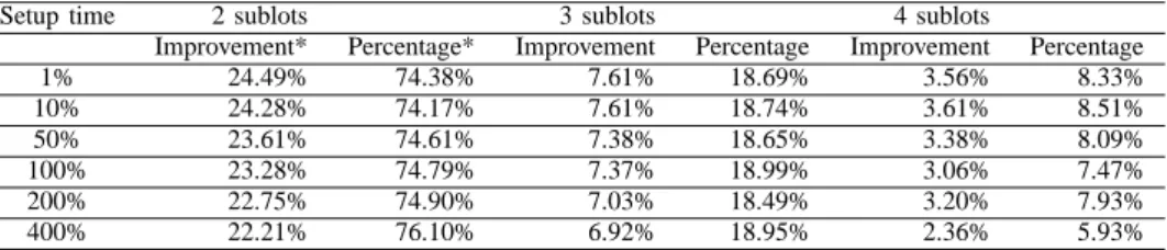
TABLE IV
PERFORMANCE OF LOT STREAMING WITH VARIOUS SETUP TIMES
Setup time 2 sublots 3 sublots 4 sublots
Improvement* Percentage* Improvement Percentage Improvement Percentage
1% 24.49% 74.38% 7.61% 18.69% 3.56% 8.33%
10% 24.28% 74.17% 7.61% 18.74% 3.61% 8.51%
50% 23.61% 74.61% 7.38% 18.65% 3.38% 8.09%
100% 23.28% 74.79% 7.37% 18.99% 3.06% 7.47%
200% 22.75% 74.90% 7.03% 18.49% 3.20% 7.93%
400% 22.21% 76.10% 6.92% 18.95% 2.36% 5.93%
* Improvement and percentage are calculated by:(Cmax,s−1−Cmax,s)/Cmax,1and(Cmax,s−1−Cmax,s)/(Cmax,1−Cmax,4), respectively.
Cmax,srepresents the makespan obtained by applyingssublots.
Makespan Improvement
Setup time (%) 25%
20%
1% 10% 50% 100% 200% 400%
Fig. 5. Makespan improvement with different setup times
B. Impact of setup times
In order to analyze the relationship between setup times and makespan reduction, we adopt the settings from [6]. The setup times are set to be 1%, 10%, 50%, 100%, 200% and 400% of the unit processing times. The computational results of 96 test instances are listed in table IV.
As plotted in figure 5, while the proportion between setup times and processing times rises, the advantage of lot stream-ing declines in accordance. Nevertheless, the improvement of makespan with 2 sublots exceeds 20%.
Evidently, there is a trade off between the time saved by splitting into sublots and the extra time required due to additional setups. Although the size of setup times imposes a negative influence on the reduction of makespan, lot streaming is still unnegligibly efficient.
C. Solutions with equal-sized sublots
As mentioned in the first section, many researches in-volved examining the performance of equal-sized sublots. In this respect, constraints (2) are modified as:
Xij =Di/s ∀i, j (19)
In comparison to solving the problem optimally, the sublot sizes are predetermined, which significantly reduces the complexity of the problem. As a result, Lingo program can be remarkably accelerated. In our study, the test instances are also solved by adopting equal-sized sublots. As presented in table V, the deviation of makespan is surprisingly only 3.05% on average, while the necessary iterations to solve identical problems fall sharply. This valuable information suggests that we can take advantage of the trade off between the reduction of computing time and the increment of makespan to solve larger instances of job shop problems. In consequence, sat-isfying solutions can be obtained within reasonable amount of time.
D. Evaluation of the formulation
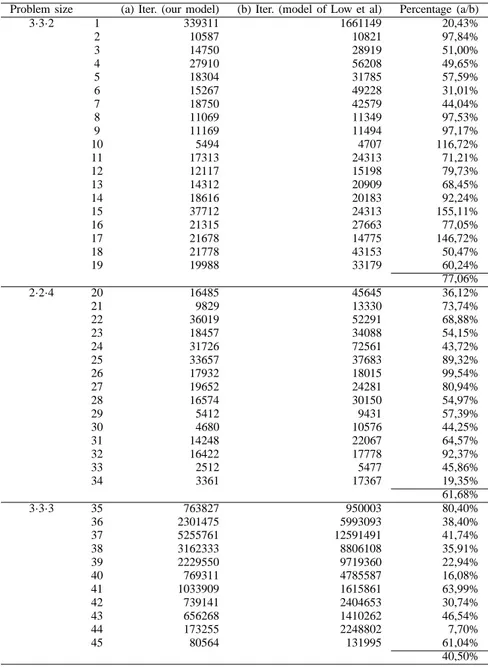
One main difference of our formulation compared to the model proposed by [8] is the successful removal of the operation index. In order to compare the efficiency of these two formulations, we implemented their model in Lingo 9.0 as well (after necessary corrections, so that feasible solutions are generated). 45 instances were tested under identical circumstances.
As shown in table VI, our formulation requires signif-icantly fewer iterations for most of the instances. This advantage becomes especially obvious when the problem size increases. The experiment confirms that our formulation is not only straightforward but also more efficient in general.
In our model constraints (17) and (18) are incorporated to describe attributes of the binary variableYiji′j′k. Constraints
TABLE V
PERFORMANCE OF EQUAL-SIZED SUBLOTS
job·machine 2 sublots 3 sublots 4 sublots Percentage *
2·3 4.11% 4.75% 4.40% 16,68%
2·4 3.40% 4.37% 4.44% 18,11%
2·5 5.78% 7.41% 7.48% 3,65%
2·6 3.09% 4.11% 4.76% 2,50%
3·3 1.91% 2.41% – 4,94%
Mean 3.05% 3.84% 4.21% 8,19%
* Percentage= iteration required applying equal sublots
iteration required applying consistent sublots
TABLE VI
COMPARISON OF THE PERFORMANCE OF TWO FORMULATIONS
Problem size (a) Iter. (our model) (b) Iter. (model of Low et al) Percentage (a/b)
3·3·2 1 339311 1661149 20,43%
2 10587 10821 97,84%
3 14750 28919 51,00%
4 27910 56208 49,65%
5 18304 31785 57,59%
6 15267 49228 31,01%
7 18750 42579 44,04%
8 11069 11349 97,53%
9 11169 11494 97,17%
10 5494 4707 116,72%
11 17313 24313 71,21%
12 12117 15198 79,73%
13 14312 20909 68,45%
14 18616 20183 92,24%
15 37712 24313 155,11%
16 21315 27663 77,05%
17 21678 14775 146,72%
18 21778 43153 50,47%
19 19988 33179 60,24%
77,06%
2·2·4 20 16485 45645 36,12%
21 9829 13330 73,74%
22 36019 52291 68,88%
23 18457 34088 54,15%
24 31726 72561 43,72%
25 33657 37683 89,32%
26 17932 18015 99,54%
27 19652 24281 80,94%
28 16574 30150 54,97%
29 5412 9431 57,39%
30 4680 10576 44,25%
31 14248 22067 64,57%
32 16422 17778 92,37%
33 2512 5477 45,86%
34 3361 17367 19,35%
61,68%
3·3·3 35 763827 950003 80,40%
36 2301475 5993093 38,40%
37 5255761 12591491 41,74%
38 3162333 8806108 35,91%
39 2229550 9719360 22,94%
40 769311 4785587 16,08%
41 1033909 1615861 63,99%
42 739141 2404653 30,74%
43 656268 1410262 46,54%
44 173255 2248802 7,70%
45 80564 131995 61,04%
1 23 4 5 6 7 8 9 1011 12 13 14 15 16 17 18 19 2021 22 23 24 25 26 27 28 29 30 31 32 33 34 35 36 37 38 3940 41 42 43 44 45 46 47 4849 50 51 52 53 54 55 56 57 58 59 60 0,00
0,50 1,00 1,50 2,00 2,50 3,00 3,50 4,00 4,50 5,00 5,50
instance
c
o
e
ff
ic
ie
n
t
coefficient= Iterations required employing (17) and (18)Iterations required without (17) and (18)
Fig. 6. Performance of (17) and (18)
were tested. The results are depicted in figure 6 where the coefficient calculation is given as well.
By employing these constraints, the necessary iterations for some instances, on the one hand, can be reduced to less than 50%. On the other hand, solving some instances with these constraints demands exceedingly more iterations. Unlike in a flow shop environment, no conclusive behaviour pattern of these constraints was recognizable.
IV. CONCLUSION
This paper addresses solving the lot streaming problem in a job shop environment, where setup times are included. The proposed integer programming formulation sufficiently describes the processing dynamics of individual sublots and enables the simultaneous determination of schedules on machines and sublot sizes. In view of setup times, various types of setups are incorporated. The model is then further developed to fulfil the requirements of special production systems.
Computational results confirm that the makespan can be considerably improved, when lot streaming techniques are applied to the standard job shop problem. Furthermore, detailed analysis is conducted to reveal the relation be-tween setup times and makespan reduction. Although the improvement of makespan declines as setup times increase, lot streaming is still advantageous.
In comparison to the model established by [8], our formu-lation is not only straightforward but also more efficient in general. However, by the implementation of the optimization-based software Lingo 9.0, only small instances of the job shop problem can be optimally solved within a realistic time span. Thus, the development of effective heuristics to solve large instances of the problem is desirable for future study. For instance, the implementation of metaheuristic is advisable.
ACKNOWLEDGMENT
The authors would like to thank the anonymous referees for their supportive comments on this paper.
REFERENCES
[1] K.R. Baker. Lot Streaming in the Two-Machine Fflow Shop with Setup Times, Annals of Operations Research, vol. 57, pp.1-11, 1995. [2] D. Biskup and M. Feldmann. Lot Streaming with Variable Sublots:
An Integer Programming Formulation, Journal of Operational Research
Society, vol. 57, pp. 296-303, 2006.
[3] U. Buscher and L. Shen. An Integrated Tabu Search Algorithm for the Lot Streaming Problem in Job Shops, European Journal of Operational
Research, vol. 19, pp. 385-399, 2009.
[4] J. Chen and G. Steiner. Lot Streaming with Attached Setups in Three-Machine Flow Shops, IIE Transactions 30, pp. 1075-1084, 1998. [5] J. Chen and G. Steiner. On Discrete Lot Streaming in No-Wait Flow
Shops, IIE Transactions, vol. 35, pp. 91-101, 2003.
[6] S. Dauz`ere-P´er`es and J.B. Lasserre. Lot Streaming in Job-Shop Schedul-ing. Operations Research, vol. 45, pp. 584-595, 1997.
[7] M. Feldmann and D. Biskup. On Lot Streaming with Multiple Products. Discussion paper, No. 542, Department of Business Administration and Economics, Bielefeld University, Germany 2005.
[8] C. Low, C.M. Hsu and K.I. Huang. Benefits of Lot Splitting in Job-Shop Scheduling, International Journal of Advanced Manufaturing
Technology, vol. 24, pp. 773–780, 2004.
[9] C.N. Potts and K.R. Baker. Flow Shop Scheduling with Lot Streaming,
Operations Research Letters, vol. 8, pp. 297-303, 1989.
[10] R.G. Vickson and B. E. Alfredsson. Two- and Three-Machine Flow Shop Scheduling Problems with Equal Sized Transfer Batches,