doi: 10.1590/0101-7438.2017.037.02.0311
MATHEMATICAL MODELLING AND SOLUTION APPROACHES FOR PRODUCTION PLANNING IN A CHEMICAL INDUSTRY
Artur Lovato Cunha and Maristela Oliveira Santos
∗Received September 01, 2016 / Accepted June 28, 2017
ABSTRACT.This paper addresses a lot sizing problem in a Brazilian chemical industry where a product can be produced by more than one process, which can use different parallel machines and may even con-sume a wide range of raw materials. Moreover, most of the products are liquids and the inventories must be kept in a restricted number of storage tanks with a limited capacity. Hence, these two issues are barely addressed in the literature on lot sizing. The classical multi-level capacitated lot sizing problem was ex-tended to address them and a mixed integer programming (MIP) formulation was developed to determine how many batches should be produced and in which tank products should be stored to meet the demands and minimize production costs. The results of computational experiments show that the commercial solver found poor quality solutions or could not find feasible solutions within one hour. Thus, we applied relax-and-fix and fix-and-optimize MIP based heuristics and we observed that these heuristics were able to obtain feasible solutions for more instances in shorter computational times and find better solutions than those obtained by the commercial solver to solve the proposed model.
Keywords: Lot sizing problem, Mixed integer programming problem, Chemical industry, Relax-and-fix, Fix-and-optimize.
1 INTRODUCTION
Production planning is one of the most important decision-making levels in the manufacturing industry and can be considered an essential tool tool to improve its (Li, Gao, Shao, Zhang & Wang, 2010) operating activities and one of the main keys to a company’s success. The lot siz-ing problem is one of the production plannsiz-ing activities and it aims to determine the production quantity and time to satisfy the demand and minimize total production costs (Yanasse, 2013). A wide variety of characteristics has been explored in this problem, such as single or multiple items, single-level or multi-level production, storage and production capacity restrictions, setup
*Corresponding author.
time and/or cost, batch production, among others. When lot sizing is performed in a batch pro-duction system, the amounts to be produced are determined as integer multiples of the batch reaction volume.
According to Karimi, Ghomi & Wilson (2003), single-level production systems produce end items directly from purchased or raw materials. Several studies have discussed the single-level capacitated lot sizing problem (CLSP) using different solution approaches, as discussed in Jans & Degraeve (2008) and Yanasse (2013). On the other hand, multi-level production systems show a parent-component relationship among items, in which the item produced in an operation can be the input of another operation (Karimi et al., 2003). Billington, McClain & Thomas (1983) were pioneers regarding the discussion on the multi-level capacitated lot sizing problem (ML-CLSP) and after their work, many studies emerged. Tempelmeier & Derstroff (1996) applied Lagrangian relaxation and Akartunali & Miller (2009) proposed a heuristic that uses LP-and-fix and relax-and-LP-and-fix for an MLCLSP with overtime. Sahling, Buschkuhl, Tempelmeier & Hel-ber (2009) treated an MLCLSP with a setup carry-over using a fix-and-optimize heuristic while Chen (2015a) used a fix-and-optimize heuristic and a variable neighborhood search (VNS). Furlan & Santos (2015) developed a hybrid approach using bees’ algorithm and fix-and-optimize. Almeder, Klabjan, Traxler & Almada-Lobo (2015) studied practical infeasibilities in production planning due to lead time assumptions. Other articles related to multi-level production systems can be found in Buschkuhl, Sahling, Helber & Tempelmeier (2010).
In the process industry, which comprises the chemical industry, production planning studies focus mainly on long-term or short-term planning. Sahinidis, Grossmann, Fornari & Chathrathi (1989) developed a mixed integer problem (MIP) model for long-term planning that considers expan-sions or shutting down production lines. Bl¨omer & G¨unther (1998) presented an MIP model to minimize the makespan for the scheduling problem with batch and multi-level systems. Grunow, G¨unther & Lehmann (2002) studied the production planning problem in a pharmaceutical and chemical industry with a batch and multi-level production line system. Cooke & Rohleder (2006) dealt with the lot sizing and scheduling problems of an industry with continuous processing and multiple plants to regulate inventory levels and quantities produced in each plant. Velez, Sun-daramoorthy & Maravelias (2013) developed an algorithm to calculate lower bounds of necessary tasks that are used to express valid inequalities to enhance MIP scheduling model performance of chemical manufacturing facilities. Mostafaei & Ghaffari Hadigheh (2014) developed an MIP model for long-term scheduling in a pipeline system of a refinery and its distribution centers. Shaik & Bhat (2014) studied short-term scheduling in a pulp industry providing a mathematical model based on a state-task-network (STN). Moniz, Barbosa-P´ovoa, de Sousa & Duarte (2014) proposed an MIP model to integrate scheduling and decision-making processes to solve a real problem from a chemical-pharmaceutical industry. Almada-Lobo, Clark, Guimar˜aes, Figueira & Amorim (2015) and Copil, W¨orbelauer, Meyr & Tempelmeier (2016) discussed various indus-trial environments and applications.
not been yet considered, covering mid-to short-term decisions which still has not been widely studied in processing industry problems. The problem was motivated by a Brazilian chemical industry and, thus can be applied in other chemical or even process industries. In the problem addressed in this paper, there are multiple machines or production units for a batch production in a system’s multi-level product structure. A feature in the problem, not common in the lot sizing problem, is the presence of multiple processes to produce an item, i.e., one product can be made following several recipes. Related research was developed by Luche, Morabito & Pureza (2009) which integrates the process selection and single-level lot sizing to tackle a production prob-lem in an electrofused grain industry where each process (or lot) can produce a set of products. However, in our paper, each process produces only one product and processes that produce the same product can differ in terms of some raw materials consumed. When a process finishes, the intermediate product is consumed in other processes or it is stored in tanks, while most of the final products must be packed. Classical lot sizing problems do not take into account inventory storage tank constraints during the production process of intermediate and final products (see Karimi et al. (2003), Chen (2015a), Furlan & Santos (2015)). The need to consider storage tanks resembles the in terms of proposed by Toledo, Franc¸a, Morabito & Kimms (2007) for the soft drink industry and Baldo, Santos, Almada-Lobo & Morabito (2014) for the brewery industry, respectively.
Therefore, in this paper, we deal with a multi-level lot sizing problem where an item can be produced adopting several processes with limited resources for production and storage of items. The problem was modelled as a mixed integer programming and a CPLEX 12.5 optimization solver was used to solve it. However, the commercial solver was not efficient in finding feasible solutions of good quality. To overcome this inefficiency, we developed relax-and-fix and fix-and-optimize heuristics, which have shown promising results for the instances generated based on real data.
2 PROBLEM DEFINITION
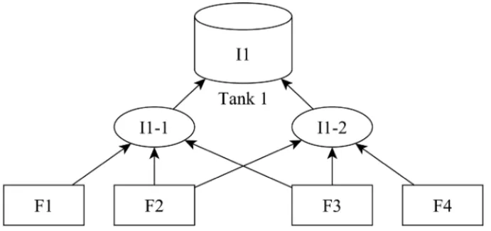
This study focuses on the medium-term production planning based on a Brazilian chemical indus-try. The production structure is characterized by the fact that more than one recipe can produce the same product, even if they consume different feedstocks. This can be seen in many chemical industries as shown in Crama, Pascual & Torres (2004) and in other process industry companies. Figure 1 illustrates an example where product I1 can be produced by two recipes (I1-1 and I1-2). Both consume feedstock F2 and F3, however recipe I1-1 uses feedstock F1 while I1-2 uses F4. The difference between the ingredients used in the recipes to produce the same product is ex-plained by the chemical similarity between the compounds, i.e., the components can be different types of alcohols (varying on the number of CH2presented in the molecule), glycols (such as
Figure 1–An example of a product that can be produced by two recipes using different feedstocks.
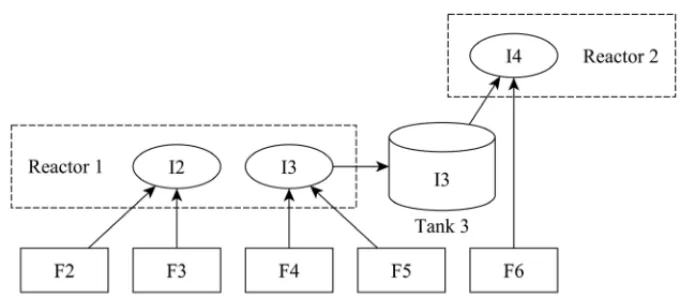
Another important feature for the chemical industry is the inventory control, which is more com-plex than what is usually dealt with in classical lot sizing problems. Products must be kept in a limited number of storage tanks for future consumption in other recipes, therefore it is important to control which product is being stored in each tank. That is because the total amount of inven-tory at the end of each period cannot be constrained only by the summation of the tanks’ capacity since products cannot share one storage tank simultaneously. Figure 2 illustrates this situation, where the inventory of products I1 and I2 do not fulfill the storage capacity, however no other product can be stored in Tank 1 and Tank 2 until they are emptied and cleaned.
Figure 2–Storage operation of a product requires exclusivity of the tank and maynot fill it completely.
Figure 3–Production process flow for two reactors of the studied industry.
After the production process finishes, products have to be packed before being delivered to cus-tomers. The packing equipment can be supplied by the tanks and reactor, since the pipes connect all of them, as illustrated in Figure 4. In fact, each reactor has a specific tank with the same capacity as its own, which can buffer products while the next batch is being processed. These dedicated tanks are assumed as an internal compound of the reactor.
Figure 4–Packing operations can receive products from reactors or from tanks.
3 MATHEMATICAL MODELLING
3.1 Modelling Assumptions
The problem described in Section 2 will not be completely modelled in this section. The reason for this is to reduce the computational burden, as well as the number of modelled features. The proposed model does not consider the availability and inventory of feedstocks, instead of that it can be used to infer the amount of feedstocks that should be purchased over the planning periods. Furthermore, the capacity of the packing equipment is large enough to not become a bottleneck of the system, so that packing operations are overlooked.
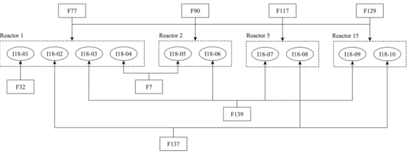
Figure 5–Example of feedstocks consumed in the production of product I18.
cannot be applied to this problem due to two main reasons: multiple recipes and storage control. Figure 5 illustrates ten different recipes used to produce product I18. These recipes are directly associated with the reactors (which from now on will be referred to as machines), that is, given a recipe number it is simple to determine in which machine this recipe has to be processed. It can be observed that feedstocks F77, F90, F117, and F129 are consumed by all recipes while feedstocks F7, F32, F137, and F139 can be used in only some recipes. Therefore, if the recipes of this product were aggregated in one product, the planning would determine how much of these last four feedstocks is necessary to meet the demand of product I18. On the other hand, the number of intermediate products kept in storage tanks is indispensable as it should be limited to the amount of storage tanks available. In addition, it is necessary to control the quantity of each designated product for the storage tank, ensuring that its limits are not violated, and thus ensuring that the solutions found are similar to those used in practice.
3.2 Mathematical Model
To model the problem, consider Jitems, indexed by j (j ∈ {1, . . . ,J}), which can be final or intermediate products to be produced over a finite planning horizon of T periods, indexed byt
(t ∈ {1, . . . ,T}). The products can be stored inQstorage tanks, indexed byq(q ∈ {1, . . . ,Q}), that are used preferably by intermediate products. The number of recipes for a product j varies from 1 to|R(j)|. Each recipercan consume one or more of theFavailable feedstocks, indexed by f (f ∈ {1, . . . ,F}), and must be processed in one of theM capacitated machines, indexed bym(m∈ {1, . . . ,M}).
In the model, there are two sets of binary variables: the first one represents setup occurrence (Yj,r,t,∀j,r,t) and the other represents tank utilization (Zq,j,t,∀q,j,t). Another set of variables
consists of integer variables which represent the number of produced batches (Xj,r,t∀j,r,t) and
the elements of the last set are continuous variables (Ij,t∀j,t) representing the inventory of
The internal demands are not multiples of production batches, therefore if the quantity of an intermediate item produced has not been completely consumed, it should be stored in a tank. However, these tanks are scarce resources and cannot be shared simultaneously by more than one product. To overcome the shortage of storage tanks, the industry allows a secondary form of storage, in which barrels can store products after a manual packaging process. Therefore, this feature has been taken into account in the model, represented by a continuous set of variables
Wj,t,∀j,t. As one of the objectives is to reduce the use of these barrels, a penalty was added to
the objective function to avoid the occurrence of this operation.
The subsets, parameters and variables considered in the mathematical model proposed are intro-duced as follows:
Subsets
F(r) feedstocks consumed by reciper;
J1(m) products that can be produced in machinem; J2(q) products that can use storage tankq; K products that can be stored in tanks; Q(j) storage tanks that can be used by product j; R(j) recipes that can produce product j.
Parameters
am,j,r consumption of machinem, in hours, for the production of one
batch of product jthrough reciper;
bq storage capacity of tankq;
cf,j,r,t cost of feedstock f to produce one batch of productj using
reciperin periodt;
dj,t demand of product jin periodt;
ej,r quantity of product j produced per batch through reciper;
gi,j,r quantity of intermediate producti consumed in the production of
one batch of product jthrough reciper;
hj,t cost of holding product jin periodt;
Ij initial inventory of product j;
sj,t setup cost of product jin periodt;
C APm,t production capacity, in hours, of machinemin periodt;
BIG M sufficiently large number;
Variables
Ij,t inventory of product jat the end of periodt;
Wj,t quantity of product j for secondary storage in periodt;
Xj,r,t batches of product jproduced by reciperin periodt;
Yj,r,t (binary) occurrence of setup for product j through reactionr, in periodt;
Zq,j,t (binary) utilization of tankq by productj at the end of periodt.
Mathematical Model
minimize
J
j=1
T
t=1
r∈R(j)
⎛
⎝
f∈F(r)
(cf,j,r,t ·Xj,r,t)+sj,t ·Yj,r,t
⎞
⎠
+(hj,t·Ij,t+β·Wj,t)
(1)
subject to
j∈J1(m)
r∈R(j)
(am,j,r ·Xj,r,t)≤C APm,t ∀m,t (2)
Ij,t−1+
r∈R(j)
(ej,r ·Xj,r,t)=dj,t
+
J
i=1
r∈R(i)
(gj,i,r ·Xi,r,t)+Wj,t+Ij,t, ∀j,t (3)
Xj,r,t ≤BIG M·Yj,r,t ∀ j,r∈R(j),t (4)
Ij,t ≤
q∈Q(j)
bq·Zq,j,t, ∀ j∈K,t (5)
Ij,0=Ij, ∀ j (6)
j∈{K∩J2(q)}
Zq,j,t ≤1, ∀q,t (7)
Ij,tandWj,t ≥0, ∀ j,t (8)
Yj,r,t andZq,j,t ∈ {0,1}, ∀ j,r∈R(j),t,q (9)
Xj,r,t ≥0 and integer, ∀ j,r∈R(j),t (10)
The secondary storage cost is calculated from the total volume for the barrel when this oper-ation is conducted.
Constraints (2) define the restrictions of the production capacity of machines. Constraints (3) express the inventory balance, i.e., the production of all recipes for a product in a period plus the stock from the previous period should be enough to meet the demands (internal and external) and the excess is held in tanks or secondary stock. Constraints (4) indicate a setup state for a recipe of a product in all periods of the planning horizon.
Constraints (5) indicate a product inventory, which can be distributed among several tanks in subsetQ(j)at the end of a period. The inventories of each product are limited to the total capacity of the tanks reserved for them. Products that do not use storage tanks, have their stocks set to zero. Constraints (6) define the initial inventory of intermediate and final products. Moreover, constraints (7) assure each tank can be used at most by one product belonging to subsetJ(q)at the end of each period. Finally, (8), (9) and (10) define the domains of variables.
4 SOLUTION APPROACHES
Two classical relax-and-fix heuristics were used aiming to find good quality solutions while other two fix-and-optimize heuristics were used intending to improve incumbent solutions.
4.1 Relax-and-fix heuristic
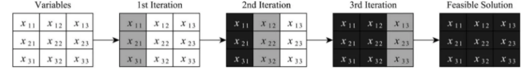
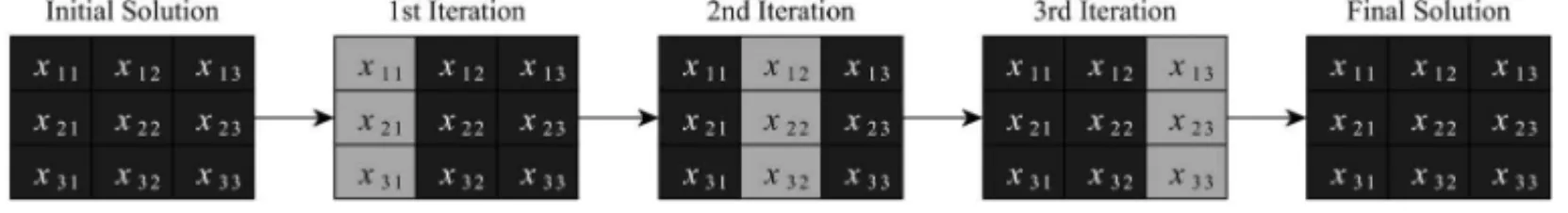
The relax-and-fix approach, proposed by Dillenberger, Escudero, Wollensak & Zhang (1994), is a constructive heuristic that partitions a problem into several subproblems containing far fewer integer variables and solves them iteratively. Basically, it divides the model variables into three disjoint subsets: fixed variables, integer (binary) variables, and relaxed variables. This heuristic has been applied to several models and presented good results (Dillenberger et al., 1994; Stadtler, 2003; Akartunali & Miller, 2009; Toledo, da Silva Arantes, Hossomi, Franc¸a & Akartunali, 2015).
Figure 6–Representation of a relax-and-fix heuristic.
variables. This second subproblem is then solved and, if a feasible solution is found, the integer variables must also be fixed one more time. In the last iteration, the third column becomes the integer variables and if this subproblem provides a feasible solution, it is also a feasible solution for the original MIP, because all integer variables of the MIP assume integer values. However, if a feasible solution cannot be found for one of the subproblems, the heuristic ends. The inability of this heuristic to find a feasible solution does not mean there is no solution.
Relax-and-fix by period (R Fp). Integer variables are partitioned according to periods. Subsets
of simplified variables usually become integers in a forward or backward sequence, from the first to the last period or from the last to the first period, respectively.
Relax-and-fix by product (R Fi). Variables are partitioned according to products. Batch
prob-lems with a multi-level product structure should start from products belonging to the highest levels because the internal demand of one level is completely known only after the demand of the higher level has been determined.
4.2 Fix-and-optimize heuristic
The fix-and-optimize approach, proposed by Helber & Sahling (2008) and then published by Helber & Sahling (2010), was originally developed as a constructive heuristic for the MLCLSP problem with overtime. Initially, the setup was assigned to each product in all periods and the heuristic was responsible for solving subproblems to optimality, avoiding unnecessary setups. However, fix-and-optimize is currently considered an improvement heuristic that requires an initial feasible solution. Fix-and-optimize has performed well in lot sizing problems, as reported by Sahling et al. (2009), Helber & Sahling (2010), Seeanner, Almada-Lobo & Meyr (2013), Xiao, Zhang, Zheng & Gupta (2013) & Chen (2015b).
Figure 7–Representation of a fix-and-optimize heuristic by period.
Basically, fix-and-optimize consists of searching for the best feasible solutions from an initial so-lution already known, thus it can be integrated with relax-and-fix heuristics (Stadtler & Sahling, 2013). Figure 7 illustrates this heuristic, which is similar to the relax-and-fix heuristic, except there are no relaxed variables. In each iteration, a subset of variables is considered integer, while the other variables remain fixed with the values of the incumbent solution. The grey and black columns represent integer and fixed variables, respectively. At the end of the iteration, if a better solution has been found, the subset of integer variables are fixed, so that another subproblem can be re-optimized. Fix-and-optimize can also partition its variables by period (F Op) and by
5 COMPUTATIONAL EXPERIMENTS 5.1 Generation of Instances
The real problem in the chemical industry deals with 281 products (of which 101 are intermedi-ate), each one with at most 12 recipes (which results in a total of 534 recipes), 49 feedstock, 7 ma-chines. The structure was kept as in the company, i.e., the processing time, production quantity and machines were maintained for each recipe feedstocks and intermediate products consumed. On the other hand, data of 12 weeks containing information about feedstock cost, external de-mand, initial stock and the storage capacity of some tanks were used to generate instances so as to simulate several scenarios similar to the ones provided by the company.
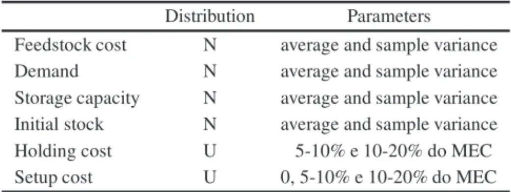
Table 1–Statistical distributions and parameters used in the data generation. Distribution Parameters
Feedstock cost N average and sample variance Demand N average and sample variance Storage capacity N average and sample variance Initial stock N average and sample variance Holding cost U 5-10% e 10-20% do MEC Setup cost U 0, 5-10% e 10-20% do MEC
The average and sample variances of the initial stock, demands, feedstock costs and storage capacity were taken from the data and applied to a normal distribution (N) to generate values for the instances. Finally, setup and storage costs were calculated according to a uniform distribution (U) and a percentage of the most expensive cost (MEC) among all recipes of each product. Table 1 summarizes the distributions and parameters used for the data generation.
According to data provided by the industry, some feedstock costs and demands of the products can be constant or variable during the planning horizon. The latter may even assume null demand in some periods, therefore around 50% of the products presented demand. Therefore, after the initial data generation (see Table 1), a new procedure was applied to increase the similarity between the generated data and data from the company.
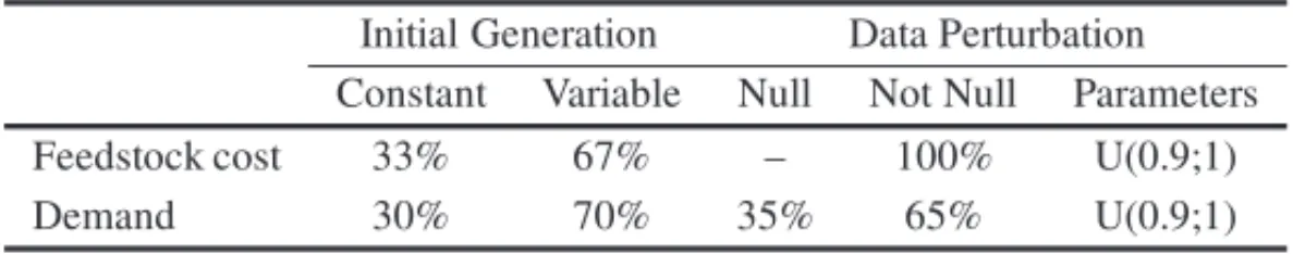
This correction procedure uses uniform distribution to determine whether the generated data must be constant or variable over the planning horizon. In the case of variable data, another uniform distribution determines if the value should be zero or assume a perturbation of the current value. This perturbation is given by the multiplication of the generated data by a uniform distribution U(0.9;1). The parameters considered are shown in Table 2 and reflect what was observed in the company’s data.
Table 2–Parameters used in the adjustment of feedstock cost and demand. Initial Generation Data Perturbation Constant Variable Null Not Null Parameters Feedstock cost 33% 67% – 100% U(0.9;1)
Demand 30% 70% 35% 65% U(0.9;1)
and 65% chance of being set to a value obtained by perturbing the base demand with a uniform distribution U(0.9;1).
The simulation of a storage tank considered 3 scenarios: one with only exclusive tanks, another in which two products share one tank and the last in which 4 products share the same tank, totalizing 101, 52 and 26 tanks, respectively. Since the initial stock was generated by a normal distribution, it may be greater than the storage capacity of the product. In this case, the initial stock of the product is defined as this storage limit. In scenarios where tanks are shared, only one of the products that use the tank has initial stock. Besides that, most of final products must be packed directly from the reactor, while all intermediate products can use storage tanks.
The procedure to determine the production capacity of machines starts by determining the sum of the time required for all recipes of a machine to attend their demand. In this step, the external demand, ordered by clients, is equally divided between all recipes of a product and the lowest integer number of batches is found to satisfy their demand portion. Therefore, the internal de-mand required for the production of other products can be equally divided once again among all recipes. The lowest integer number of batches is then updated to satisfy the total demand of all recipes. Finally, the production capacities are disturbed from the last to the second periods, following a uniform distribution U (0.9, 1.0). The reduced capacity in each period is added to the previous period to avoid infeasibility. Two variations, a tighter one (110%) and another looser (125%), based on the productive capacity are then generated.
The final instances consist of ten subsets generated and based on a structure of product, reactions, and machines. Each subset has one value of demand and feedstock cost, two values of periods (6 and 12 weeks), holding costs and production capacity, and three values of setup cost and storage tanks. Therefore, 720 instances were generated for use in the computational experiments.
5.2 Execution Analysis
The computational experiments were performed using the optimization CPLEX 12.5 package, on a computer with a Linux Mint 15 operating system, an IntelR CoreTMi7-2600 processor and
16 GB of RAM. The following settings of CPLEX were changed: one thread for each execution, relative GAP of 10−6and time limit of 3600 seconds. The models built to represent each instance have at most 6408 integer, 7620 binary and 3473 continuous variables. The combined heuristics have a different time limit: relax-and-fix by period with fix-and-optimize by period (R FpF Op)
phase while relax-and-fix by period with fix-and-optimize by item (R FpF Oi) have 3240 and
360 seconds, respectively. These heuristics split the total available time equally among their subproblems, i.e.,R FpF Opdesignated 150 seconds for each iteration ofR FpandF Opphases,
for instances with 12 periods, while 300 seconds for instances with 6 periods.
Mathematical Model
First, we evaluated the performance of CPLEX in solving the MIP model for all proposed in-stances. After one hour of execution, feasible solutions were found in 85% of the instances with six periods in the planning horizon and in 70% of the instances with 12 periods. The average GAPs, calculated by
100∗feasible solution – lower bound lower bound
,
were higher than 20% and the average execution times were more than 3583 seconds.
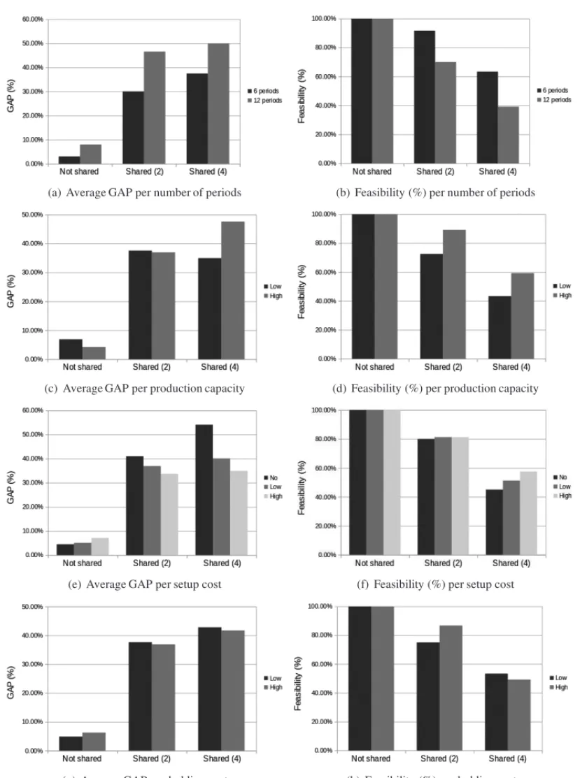
Figure 8 shows some graphics of the quality of solutions and feasibility percentage according to the number of periods, production capacity, setup and holding costs for not shared and shared tanks. An overview of the behavior of the solutions shows their quality, measured by the average GAP, deteriorates from not shared to shared tanks, as well as from two to four products shar-ing the same tank. In the same situation, the number of feasible solutions found by the solver decreases.
When the number of periods increases, the average GAPs become higher and the percentage of feasible solutions reduces, as shown in Figures 8(a) and 8(b), because the number of variables in the MIP model increases when the number of periods changes from 6 to 12.
Instances of a looser production capacity enable the optimization package to find more feasible solutions than those with a tighter capacity, as shown in Figure 8(d). However, the optimiza-tion package faces difficulties in finding soluoptimiza-tions of good quality or proving their quality when storage tanks change from not shared to shared or when the shared level increases. Especially instances with higher production capacity show such a behavior, as shown in Figure 8(c).
According to Figure 8(e), the average GAPs of instances with not shared tanks increase when the setup costs rise. On the other hand, average GAPs of instances with shared tanks decrease when the setup costs increase, which indicates that the optimization solver can explore solutions more efficiently, raising lower bounds of the MIPs. Figure 8(f) shows that higher setup costs help the solver to obtain feasible solutions for instances with 4 products sharing the same tank, whereas, for other instances, the feasibility percentages are almost identical when the setup costs vary.
(a) Average GAP per number of periods (b) Feasibility (%) per number of periods
(c) Average GAP per production capacity (d) Feasibility (%) per production capacity
(e) Average GAP per setup cost (f) Feasibility (%) per setup cost
(g) Average GAP per holding cost (h) Feasibility (%) per holding cost
Heuristics
We used relax-and-fix by period (R Fp), relax-and-fix by product (R Fi), fix-and-optimize by
period (F Op), fix-and-optimize by product (F Oi) and some of its combinations, as shown in
Table 3, to overcome the difficulty faced by the optimization package regarding the resolution of the mathematical model. As relax-and-fix by product (R Fi) and relax-and-fix by product with
fix-and-optimize by period (R FiF Op) were not promising for the instances considered in the
tests, their results will be omitted in future analyses.
Table 3–Heuristics used in the computational experiments. Relax-and-fix Fix-and-optimize Period Item Period Item
R Fp – – –
R FpF Op – –
R FpF Oi – –
R FiF Oi – –
In general, R Fi divides MIP into several subproblems with few integer variables, at most 144
integer and 156 binary, and 22.8 integer and 34.8 binary on average. Therefore, near-optimal so-lutions can be quickly found for each subproblem. However, the subproblems for instances with shared tanks represent the original problem more weakly thanR Fp, because in each iteration the
whole planning horizon of a single product is fixed. One consequence of this procedure is that some tanks can be allocated improperly during the first iterations. This may happen due to the relaxedZq,j,t variables, which allow more than one product to use a single tank simultaneously,
which is forbidden in practice. During the iterations, variablesZq,j,t become integer again and
require exclusivity of the storage tank, which can lead to unavailable tanks in some period that still may need to store products. This drawback is dealt with directly in theR Fpapproach, since
allZq,j,t variables of one period are considered integer in each iteration.
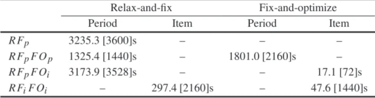
Table 4 shows the average and maximum execution times spent on each heuristic. The divi-sion of time used in the constructive and improvement phases considers only one iteration for the fix-and-optimize, which simplifies the control of the execution time limit. However, other approaches, as a total number of iterations, could have been used.
Table 4–Average [maximum] execution time in seconds for the heuristics. Relax-and-fix Fix-and-optimize
Period Item Period Item
R Fp 3235.3 [3600]s – – –
R FpF Op 1325.4 [1440]s – 1801.0 [2160]s –
R FpF Oi 3173.9 [3528]s – – 17.1 [72]s
Analysis of results
Table 5 provides information about the number of feasible and best solutions found by the exper-iments, as well as GAPs and average times, of 360 instances with a planning horizon of 6 periods and 360 instances with 12 periods. R FpF Oi showed the best performance, in the test set, and
R Fp showed good performance. The former provided the largest number of feasible solutions
and lowest average, maximum and minimum GAPs. However, the differences in the average GAP between R Fp andR FpF Oi were only 0.02% for instances with 6 periods and 0.06% for
instances with 12 periods.
Table 5–Results for tests with 3600 seconds.
Periods MIP R Fp R FpF Op R FpF Oi R FiF Oi
Feasible Sol.
6
306 360 360 360 323
Best Solutions 0 84 19 195 43
Average GAP 21.32% 1.66% 1.73% 1.64% 7.33% Maximum GAP 87.86% 4.12% 4.36% 4.05% 22.20% Minimum GAP 0.67% 0.52% 0.50% 0.48% 0.51% Average Time 3583.0s 3179.4s 3122.2s 3126.2s 188.1s Feasible Sol.
12
251 360 360 360 339
Best Solutions 0 83 3 225 46
Average GAP 28.80% 2.02% 2.20% 1.96% 7.16% Maximum GAP 90.12% 6.47% 7.11% 6.00% 18.52% Minimum GAP 0.68% 0.46% 0.44% 0.43% 0.43%
Average Time 3589.7s 3291.1s 3130.6s 3255.2s 455.3s
R FpF Opwas able to find feasible solutions for all instances with intermediate quality worse
than R Fp andR FpF Oi. The MIP model and R FiF Oi heuristic were not able to find feasible
solutions for all the instances. On the other hand, R FiF Oi showed a good performance for
instances with not shared tanks, i.e., it obtained the best solution in over 35% of the instances, as shown in Table 6. However, for instances that have shared tanks, R FiF Oi found solutions
of lower quality than those found by the other heuristics and and failed in obtaining feasible solutions for some instances, as discussed in Subsection 5.2.
Table 6–Number of best solutions found by heuristics grouped by number of periods and shared tanks. Periods Max sharing MIP R Fp R FpF Op R FpF Oi R FiF Oi
6
1 0 0 10 65 43
2 0 31 2 81 0
4 0 53 7 49 0
12
1 0 0 3 71 46
2 0 45 0 74 0
The good performance of R Fp is due to the large production capacity of the instances in
ear-lier periods and to the reasonable number of integer variables in each MIP subproblem. The distribution of production capacity through periods meets the demand in later periods with the consumption of inventory. On the other hand, the number of integer variables in the subproblems enables the optimization package to perform well in reasonable time. Finally, the efficiency of
R FpF Oi is due mainly to the constructive phase (relax-and-fix), which can find good-quality
solutions and the improvement phase (fix-and-optimize), which can refine them.
Analysis of constructive phases
Comparing the running times and solutions obtained byR Fpand only by the constructive phase
(relax-and-fix) of theR FpF Oi revealed that longer execution time does not guarantee best
solu-tions since both use the same code but with a different time limit. Table 7 shows that the construc-tive heuristicR Fpruns approximately 60 seconds more than the constructive phase ofR FpF Oi,
which is because the latter has some reserved time for the improvement phase (fix-and-optimize). Nevertheless, the constructive phase ofR FpF Oi showed an average GAP 0.002% lower than
that ofR Fpfor instances with 12 periods.
Table 7–Comparison between the constructive phase ofR FpandR FpF Oi.
Periods Best Solution Average GAP Average exec. time R Fp Draw R FpF Oi R Fp R FpF Oi R Fp R FpF Oi
6 161 31 168 1.663% 1.664% 3179.4s 3116.2s 12 166 10 184 2.020% 2.018% 3291.1s 3231.6s
Furthermore, the constructive phase of R FpF Oi was more efficient than that of R Fp for
in-stances with 6 and 12 periods when the absolute number of best solutions was considered (see Table 7). Although it seems counter-intuitive, since we expected the constructive phase to per-form better over more time, it stimulated us to investigate the influence of reducing the execution time on the final values of feasible solutions.
Analysis of the influence of the execution time
The aim of this part of the experiments was to analyse how the execution time influences the quality of solutions found by MIP, R Fp andR FpF Oi. The total time for each experiment was
limited to 36, 72, 144 and 288 seconds. However, R FpF Oi was not able to perform the tests
with 36 seconds for instances with 12 periods due to the shortage of processing time, since in this case theF Oiphase requires at least 26 seconds to perform all subproblems, leaving less than
1 second to perform each subproblem of theR Fpphase.
Table 8–Average GAPs of the feasible solutions found when the number of periods and execution time were varied.
Periods Execution time
36s 72s 144s 288s 3600s MIP
6
38.44% 34.84% 26.94% 25.08% 21.32% R Fp 5.48% 3.86% 3.03% 2.37% 1.66%
R FpF Oi 3.90% 3.00% 2.60% 2.25% 1.64%
MIP
12
45.57% 43.44% 37.91% 31.03% 28.80% R Fp 10.98% 6.91% 5.16% 3.82% 2.02%
R FpF Oi – 4.62% 3.43% 2.99% 1.96%
6 CONCLUSIONS
This paper has addressed a lot sizing problem in a Brazilian chemical industry. The problem was modelled as a mixed integer programming (MIP) and aimed at minimizing costs of feedstock, setup, inventory and secondary storage. Storage tanks were modelled for intermediate products, which limits the amount of stock.
According to the computational experiments conducted, increasing the number of periods ham-pers the resolution of the problem, while increasing the holding cost exerts no significant influ-ence. When the production capacity and setup cost rise, more feasible solutions can be found. On the other hand, increasing the production capacity results in larger average GAPs, possibly due to the difficulty of finding feasible solutions of good quality or proving their quality. Finally, the average GAPs of instances that have shared tanks tend to be reduced when setup costs are higher.
The optimization solver used in the computational tests were able to find feasible solutions with average GAPs lower than 8.04% for instances with not shared storage tanks. However, for shared storage tanks, the percentage of feasibility was reduced and the average GAPs significantly in-creased, which indicates the need for heuristics to solve the proposed problem.
Among the heuristic approaches proposed, relax-and-fix by periods (R Fp) and relax-and-fix
by periods with fix-and-optimize by products (R FpF Oi) showed to be promising for problems
similar to those found in the industry under study. Both heuristics were able to find good feasible solutions with an average GAP between 1.64% and 2.02% after one hour of execution. When a shorter time was available, i.e. 36 to 288 seconds, R Fp managed to find feasible solutions for
over 99% of the instances, whileR FpF Oi showed the lowest average GAPs but found a smaller
number of feasible solutions.
One of the objectives of the industry studied is to resolve instances in a shorter time to help PCP managers to analyze several scenarios of a production plan. The heuristics addressed in this study met the industry requirements. R FpandR FpF Oi performed much better than the mixed
Further research can extend the proposed model by including setup time, production cost for each production unit, packaging capacity or incorporating scheduling of production or storage. Furthermore, other heuristics can be applied to this problem to evaluate its performance, such as a variable neighborhood search (VNS) (Almada-Lobo, Oliveira & Carravilla, 2008) or an adaptive large neighborhood search (ALNS) (Muller, Spoorendonk & Pisinger, 2012).
ACKNOWLEDGMENTS
This research was partially funded by CAPES (Coordenac¸˜ao de Aperfeic¸oamento de Pessoal de N´ıvel Superior) project no. 137425/2011-2, Fundac¸˜ao de Amparo `a Pesquisa do Estado de S˜ao Paulo (FAPESP) via CEPID No. 2013/07375-0 and CNPq (Conselho Nacional de Pesquisa).
REFERENCES
[1] AKARTUNALIK & MILLER AJ. 2009. A heuristic approach for big bucket multi-level production planning problems.European Journal of Operational Research,193(2): 396–411.
[2] ALMADA-LOBOB, CLARKA, GUIMARAES˜ L, FIGUEIRAG & AMORIMP. 2015. Industrial In-sights into Lot Sizing and Scheduling Modeling.Pesquisa Operacional,35: 439–464.
[3] ALMADA-LOBOB, OLIVEIRAJF & CARRAVILLAMA. 2008. Production planning and scheduling in the glass container industry: A VNS approach.International Journal of Production Economics,
114(1): 363–375.
[4] ALMEDERC, KLABJAND, TRAXLERR & ALMADA-LOBOB. 2015. Lead time considerations for the multi-level capacitated lot-sizing problem.European Journal of Operational Research,241(3): 727–738.
[5] BALDOTA, SANTOSMO, ALMADA-LOBOB & MORABITOR. 2014. An optimization approach for the lot sizing and scheduling problem in the brewery industry.Computers & Industrial Engineer-ing,72: 58–71.
[6] BILLINGTONPJ, MCCLAINJO & THOMASLJ. 1983. Mathematical programming approaches to capacity-constrained MRP systems: Review, formulation and problem reduction.Management Sci-ence,29: 1126–1141.
[7] BLOMER¨ F & G ¨UNTHERH-O. 1998. Scheduling of a multi-product batch process in the chemical industry.Computers in Industry,36(3): 245–259.
[8] BLOMER¨ F & G ¨UNTHERH-O. 2000. Lp-based heuristics for scheduling chemical batch processes. International Journal of Production Research,38(5): 1029–1051.
[9] BUSCHKUHLL, SAHLINGF, HELBERS & TEMPELMEIERH. 2010. Dynamic capacitated lot-sizing problems: a classification and review of solution approaches.OR Spectrum,32: 231–261.
[10] CHENH. 2015a. Fix-and-optimize and variable neighborhood search approaches for multi-level ca-pacitated lot sizing problems.Omega,56: 25–36.
[11] CHEN H. 2015b. Fix-and-optimize and variable neighborhood search approaches for multi-level capacitated lot sizing problems.Omega,56: 25–36.
[13] COPIL K, W ¨ORBELAUERM, MEYR H & TEMPELMEIERH. 2016. Simultaneous lotsizing and scheduling problems: a classification and review of models.OR Spectrum, 1–64.
[14] CRAMAY, PASCUALR & TORRESA. 2004. Optimal procurement decisions in the presence of total quantity discounts and alternative product recipes.European Journal of Operational Research,
159(2): 364–378.
[15] DILLENBERGERC, ESCUDEROLF, WOLLENSAK A & ZHANGW. 1994. Lotsizing models for production planning on practical resource allocation for production planning and scheduling with period overlapping setups.European Journal of Operational Research,75(2): 275–286.
[16] FURLANMM & SANTOSMO. 2015. Bfo: a hybrid bees algorithm for the multi-level capacitated lot-sizing problem.Journal of Intelligent Manufacturing, 1–16.
[17] GRUNOWM, G ¨UNTHERH-O & LEHMANNM. 2002. Campaign planning for multistage batch pro-cesses in the chemical industry.OR Spectrum,24(3): 281–314.
[18] HELBER S & SAHLINGF. 2008. A fix-and-optimize approach for the multi-level capacitated lot sizing problem (Tech. Rep.). K¨onigsworther Platz 1, D-30167 Hannover: Institut f¨ur Produktion-swirtschaft, Leibniz Universit¨a Hannover.
[19] HELBER S & SAHLINGF. 2010. A fix-and-optimize approach for the multi-level capacitated lot sizing problem.International Journal of Production Economics,123(2): 247–256.
[20] JANSR & DEGRAEVEZ. 2008. Modeling industrial lot sizing problems: a review.International Journal of Production Research,46(6): 1619–1643.
[21] KARIMIB, GHOMISF & WILSONJ. 2003. The capacitated lot sizing problem: a review of models and algorithms.Omega,31(5): 365–378.
[22] LIX, GAOL, SHAO X, ZHANGC & WANGC. 2010. Mathematical modeling and evolutionary algorithm-based approach for integrated process planning and scheduling.Computers & Operations Research,37(4): 656–667.
[23] LUCHEJRD, MORABITOR & PUREZAV. 2009. Combining process selection and lot sizing models for production scheduling of electrofused grains.Asia-Pacific Journal of Operational Research,26(3): 421–443.
[24] MONIZS, BARBOSA-P ´OVOAAP,DESOUSAJP & DUARTEP. 2014. Solution methodology for scheduling problems in batch plants.Industrial & Engineering Chemistry Research,53(49): 19265– 19281.
[25] MOSTAFAEIH & GHAFFARIHADIGHEHA. 2014. A general modeling framework for the long-term scheduling of multiproduct pipelines with delivery constraints.Industrial & Engineering Chemistry Research,53(17): 7029–7042.
[26] MULLERLF, SPOORENDONKS & PISINGERD. 2012. A hybrid adaptive large neighborhood search heuristic for lot-sizing with setup times.European Journal of Operational Research,218(3): 614– 623.
[27] SAHINIDISN, GROSSMANNI, FORNARIR & CHATHRATHIM. 1989. Optimization model for long range planning in the chemical industry.Computers & Chemical Engineering,13(9): 1049–1063. [28] SAHLINGF, BUSCHKUHLL, TEMPELMEIERH & HELBERS. 2009. Solving a multilevel
[29] SEEANNERF, ALMADA-LOBOB & MEYRH. 2013. Combining the principles of variable neighbor-hood decomposition search and the fix&optimize heuristic to solve multi-level lot-sizing and schedul-ing problems.Computers & Operations Research,40(1): 303–317.
[30] SHAIKMA & BHATS. 2014. Scheduling of displacement batch digesters using discrete time formu-lation.Chemical Engineering Research and Design,92(2): 318–339.
[31] STADTLERH. 2003. Multilevel lot sizing with setup times and multiple constrained resources: Inter-nally rolling schedules with lot-sizing windows.Operations Research,51(3): 487–502.
[32] STADTLERH & SAHLINGF. 2013. A lot-sizing and scheduling model for multi-stage flow lines with zero lead times.European Journal of Operational Research,225(3): 404–419.
[33] TEMPELMEIER H & DERSTROFFM. 1996. A lagrangean-based heuristic for dynamic multilevel multiitem constrained lotsizing with setup times.Management Science,42(5): 738–757.
[34] TOLEDOCFM,DASILVAARANTESM, HOSSOMIMYB, FRANC¸APM & AKARTUNALIK. 2015. A relax-and-fix with fix-and-optimize heuristic applied to multi-level lot-sizing problems.Journal of Heuristics,21(5): 687–717.
[35] TOLEDOCFM, FRANC¸APM, MORABITOR & KIMMSA. 2007. Um modelo de otimizac¸˜ao para o problema integrado de dimensionamento de lotes e programac¸˜ao da produc¸˜ao em f´abricas de refrige-rantes.Pesquisa Operacional,27(1): 155–186.
[36] VELEZS, SUNDARAMOORTHYA & MARAVELIASCT. 2013. Valid inequalities based on demand propagation for chemical production scheduling mip models.AIChE Journal,59(3): 872–887. [37] XIAOJ, ZHANGC, ZHENGL & GUPTAJND. 2013. Mip-based fix-and-optimise algorithms for the
parallel machine capacitated lot-sizing and scheduling problem.International Journal of Production Research,51(16): 5011–5028.