An Integer Programming Formulation of the
Minimum Common String Partition Problem
S. M. Ferdous1,2*, M. Sohel Rahman2
1Department of Computer Science and Engineering, Ahsanullah University of Science and Technology (AUST), Dhaka, Bangladesh,2AℓEDA Group, Department of Computer Science and Engineering, Bangladesh University of Engineering and Technology (BUET), Dhaka, Bangladesh
Abstract
We consider the problem of finding a minimum common string partition (MCSP) of two strings, which is an NP-hard problem. The MCSP problem is closely related to genome comparison and rearrangement, an important field in Computational Biology. In this paper, we map the MCSP problem into a graph applying a prior technique and using this graph, we develop an Integer Linear Programming (ILP) formulation for the problem. We implement the ILP formulation and compare the results with the state-of-the-art algorithms from the lit-erature. The experimental results are found to be promising.
1 Introduction
In the minimum common string partition (MCSP) problem, we are given tworelatedstrings (S,T). Two strings are said to be related if the frequencies of each letter in the two strings match. A partition of a stringSis defined as a sequenceP= (b1,b2,. . .,bc), wherebiare
sub-strings ofSwhose concatenation is equal toS, i.e.,b1b2. . .bc=S. Given a partitionPof a string
Sand a partitionQof a stringT, we say that the pairπ=<P,Q>is a common partition of (S, T) ifQis a permutation ofP. The minimum common string partition problem is to find a com-mon partition of (S,T) with the minimum number of substrings, that is to minimizec. For example, if (S,T) = (atatgat,atgatat), then an optimal solution isπ= {atgat,at} and the mini-mum common partition size is 2. The restricted version of MCSP where each letter occurs at mostdtimes in each input string, is denoted byd-MCSP. A more detailed study of the applica-tion of MCSP can be found in [1], [2] and [3].
In this paper, we present an Integer Linear Programming (ILP) formulation for the MCSP problem. In particular, we use a graph mapping that was presented in our prior work [4] to solve the MCSP problem using the Ant Colony Optimization technique [5]. Here we exploit this graph to devise an ILP formulation for the problem. Then we implement the ILP formulation, conduct extensive experiments and compare the results with the state-of-the-art algorithms from the liter-ature. As will be reported in a later section, the results clearly indicate that the ILP formulation is effective and provides excellent results. One of the intriguing findings of our work is the fact that our ILP formulation turns out to be more effective and accurate than our meta-heuristics
a11111
OPEN ACCESS
Citation:Ferdous SM, Rahman MS (2015) An Integer Programming Formulation of the Minimum Common String Partition Problem. PLoS ONE 10(7): e0130266. doi:10.1371/journal.pone.0130266
Editor:Lars Kaderali, Technische Universität Dresden, Medical Faculty, GERMANY
Received:July 20, 2014
Accepted:May 19, 2015
Published:July 2, 2015
Copyright:© 2015 Ferdous, Rahman. This is an open access article distributed under the terms of the
Creative Commons Attribution License, which permits unrestricted use, distribution, and reproduction in any medium, provided the original author and source are credited.
Data Availability Statement:All relevant data are within the paper and its Supporting Information files.
Funding:The authors have no support or funding to report.
approach presented in [4]. This is especially interesting because both the algorithms are based on the same graph that is constructed through an interesting mapping [4].
The rest of the paper is organized as follows. In Section 2 we present a brief literature review. Section 3 presents the notations and definitions used in this paper. In Section 4 we present the ILP formulation for the MCSP problem. We present our experimental results in Sections 5 fol-lowed by a brief relevant discussion in Section 6. Finally, we briefly conclude in Section 7.
2 Related Works
The 1-MCSP problem is essentially the breakpoint distance problem [6] between two permuta-tions, which is solvable in polynomial time [1]. The 2-MCSP problem has been shown to be NP-hard and moreover APX-hard in [1]. The authors in [1] also have presented several approximation algorithms to solve the problem. In [2], Chen et al. have studied a generaliza-tion of the MCSP problem called the Signed Reversal Distance with Duplicates (SRDD). Fur-thermore, they have presented a 1.5-approximation algorithm for the 2-MCSP problem. In [7], Damaschke has analyzed the fixed-parameter tractability of the MCSP problem considering different parameters. The MCSP problem is also studied in [8], where it is termed as the true evolutionary distance problem between two genomes. In [9], the authors have investigated the d-MCSP problem along with two other variants, namely,MCSPc, where the alphabet size is at mostcandx-balanced MCSP, which requires that the length of blocks be at mostxaway from the average length. They have shown thatMCSPcis NP-hard whenc2. As ford-MCSP, they have presented an fixed parameter tractable (FPT) algorithm which runs inO((d!)k) time, wherekis the number of blocks in the optimal common partition. The result has been improved by Bulteau et al. [10] by showing that MCSP can be solved inO(d2kkn) time. Recently, Bulteau and Komusiewicz [11] have introduced the first fixed-parameter algorithm for the MCSP problem using parameterkonly.
Chrobak et al. [3] have analyzed a natural greedy heuristic for the MCSP problem: itera-tively, at each step, it extracts a longest common substring from the input strings. They have shown that for the 2-MCSP problem, the approximation ratio (for the greedy heuristic) is exactly 3. They also have proved that for the 4-MCSP problem the ratio is lognand for the gen-eral case, it lies betweenO(n0.43) andO(n0.67). In [12], He has proposed an improved greedy algorithm based on the greedy strategy of [3], where the idea is to extract the longest common substring containing a symbol occurring only once at each step whenever there is such a symbol.
In our prior work [4], we have developed a meta-heuristc algorithm, namely, MAX-MIN ant system to solve the MCSP problem. In particular, in [4], we have mapped the instance of the MCSP problem into a graph, namely, the common substring graph. MAX-MIN Ant System has been implemented over this graph. Recently in [13], Blum et al. have proposed an iterative probabilistic tree search algorithm for solving this problem. The algorithm is an iterative prob-abilistic variant of the greedy algorithm of [3]. The authors have tested their approach with the dataset introduced in [4]. Subsequently, a common block based ILP formulation has been pro-posed in [14] by Blum et al. They have tested their ILP formulation on the previous bench-marks [4] as well as on a new benchmark of 7 larger instances.
3 Preliminaries
This section summarizes the definitions and notations used throughout the paper. Two strings (S,T), of equal length (n), over an alphabet∑are calledrelatedif the frequencies of the letters
structure whereiandjdenote the starting and ending positions of the block. A block, [S,i,j] represents a substring ofSdenoted assubstring([S,i,j]) with length (j−i+1).
As an example, if we have two strings (S,T) = (atgcat,tgcata), then [S, 0, 1] and [S, 4, 5] both represent the substringatofS. In other words,substring([S, 0, 1]) =substring([S, 4, 5]) =
at. We say that a blockBmatches with another blockB0if the two blocks represent the same substrings. Given a list of blockslb,matchList(lb,B) is defined as a list of those blocks oflbthat
matchB. For the example stated above, let a list of blocks belb= {[S, 0, 1], [S, 1, 1], [S, 4, 5]}
andB= [S, 0, 1]; thenmatchList(lb,B) = {[S, 0, 1], [S, 4, 5]}.
We use the notion of a common substring graph as introduced in [4]. A common substring graph,Gcs(V,E,S) of two strings (S,T) is defined as follows. HereVis the vertex set of the
graph andEis the edge set. Vertices are the positions of stringS, i.e., for eachv2V,v2{0,n
−1}. Two verticesvivjare connected with an edge, i.e, (vi,vj)2E, if the substring induced by
the block [S,vi,vj] matches some substring ofT. More formally, ifSTdenotes the set of all
sub-strings ofT, we have:
ðvi;vjÞ 2E, 9s2ST : substringð½S;vi;vjÞ ¼s
In other words, each edge in the edge set corresponds to ablocksatisfying the above condi-tion. For convenience, we will denote the edges asedge blocksand use the list of edge blocks (instead of edges) to define the edge setE.
For example, suppose (S,T) = (atgcta,atgcat). The corresponding common substring graph of the first stringS, denoted byGcs(V,E,S), will have vertex set,V= {0, 1, 2, 3, 4, 5} and edge
set,E= {[S, 0, 0], [S, 1, 1], [S, 2, 2], [S, 3, 3], [S, 4, 4], [S, 5, 5], [S, 0, 1], [S, 1, 2], [S, 2, 3], [S, 0, 2], [S, 1, 3], [S, 0, 3]}.
4 ILP Formulation
Suppose we are given two related strings (S,T), each of lengthn. We create two graphs, namely, Gcs(V1,E1,S) andGcs(V2,E2,T) of (S,T), whereV1andV2are the vertex sets andE1andE2are
the edge block sets of the two graphs respectively. We define two sets of binary variables, namely,xt1andyt2wheret12E1andt22E2. We also write
δ
k(v)
−
andδ
k(v)+for the sets of
incoming and outgoing edge blocks fromEkwherev2Vkandk2{1, 2}. An incoming
(outgo-ing) edge block is the one whose starting (end(outgo-ing) positioni(j) is 0 (n−1). With the above
set-ting, we develop an ILP formulation (denoted asILPgraph) for the MCSP problem using the
common substring graph as follows:
minimize X t12E1
xt1 ð1Þ
subject to X t12E1
xt1¼ X
t22E2
yt2 ð2Þ
X
t12d1ð0Þþ
xt1 ¼
1 ð3Þ
X
t12d1ðvÞ
xt1¼ X
t12d1ðvþ1Þþ
xt1 8v2 ½
X
t22d2ð0Þþ
yt2 ¼
1 ð5Þ
X
t22d2ðvÞ
yt2¼ X
t22d2ðvþ1Þþ
yt2 8v2 ½0;n 1 ð6Þ
X
b12matchListðE1;t1Þ
xb1¼
X
b22matchListðE2;t1Þ
yb2 8t12E1 ð7Þ
xt12 f
0;1g;y t2 2 f
0;1g ð8Þ
4.1 Explanation of the Formulation
Objective function. Eq 1is the objective function that is to be minimized. The function simply calculates the size of the partition.
Equality constraint. Eq 2states that two partitions on the two substring graphs must be of equal size. In other words, the number of blocks in the factorization of the first stringSmust be equal to the number of blocks in the factorization of the second stringT.
Factorization constraint. Eqs3and4together ensures that a unit flow enters at the source (the vertex labelled with 0) and arrives at the sink (the vertex labelled withn−1) for stringS.
So, the string is factorized. For stringTthe factorization is achieved in a similar fashion by Eqs
5and6. These constraints ensure that the strings get factorized by non-overlapping blocks.
One to one match constraint. We have two sets of blocks after the factorization. We must ensure that there is a one to one matching between the two sets of blocks. By matching we mean that, for each selected block (withxt= 1 wheret2E1) of the first edge block setE1, there
must be one and only one corresponding selected block (withyt= 1 wheret2E2) with the
same substring in the second edge block setE2and vice versa.Eq 7achieves the one to one
matching by ensuring that for each edge block, the number of selected blocks inE1equals the
number of selected blocks inE2.
Integrality constraint. Eq 8ensures the integrality of the variables.
This is a polynomial formulation. The number of variables as well as the number of con-straints of the formulation depends on the size of the edge block sets,E1andE2. In the worst
case, the number of variables and constraints can beO(n2), wherenis the size of the vertex set. But in practice the number of variables is much less than that which is evident from the experi-mental results as reported in the following section.
5 Experiments
5.1 Data sets
We have conducted our experiments on 5 sets of random synthetic data (henceforth labelled as Group1-Group5) and a real gene sequence dataset (henceforth labelled as Real). The datases are briefly described below.
Group1-Group3. In our previous work [4], we generated uniform random DNA sequences, each of length at most 600, using“FaBox (1.41)”[16]. A pair of DNA sequences (S, T) was generated by randomly shuffling [16] one DNA sequence from the set using“Sequence Manipulation Suite”[17]. This dataset is divided into 3 groups. The first 10 (Group1) have lengths less than or equal to 200 bps (base-pairs), the next 10 (Group2) have lengths within [201, 400] and the rest 10 (Group3) have lengths within [401, 600] bps. Notably, these datases are also used for experimentation and analysis by researchers in recent papers [13,14].
Group4. We have also tested our formulation with a new random dataset collected through personal communication with Christian Blum, one of the co-authors of [14]. This new dataset is a collection of 300 uniform random instances of different lengths and alphabet sizes. The sequences in the dataset are of lengths {100, 200, 300, 400, 500, 600, 700, 800, 900, 1000} and of alphabet size {4, 12, 20}. In particular, for each length there are 30 sequences among which the first 10 are of alphabet size 4, the next 10 are of alphabet size 12 and the rest are of alphabet size 20.
Group5. This dataset was introduced in [14] to test the solving limit of their ILP formula-tion. This constitutes 7 instances of length {800, 1000, 1200, 1400, 1600, 1800, 2000}.
Real. We have used the real gene sequence data used in [4]. This data correspond to the first 15 gene sequences of Bacterial Sequencing (part 14) whose lengths are within [200, 600].
5.2 Implementation
SCIP [15] (version 3.1.0) standalone solver is used to solve the ILP formulation. SCIP runs on single thread [18]. The solution of an instance is a two steps procedure. Firstly for each instance we have to generate the variables and constraints in a format that is understandable to SCIP. Using Matlab we have generated the MPS (Mathematical Programming System) files of the instances. These files are the input to the solver. For the solver, we have enforced a time limit of 3600 cpu seconds for Group1-Group3, Group4 and Real. The First 5 out of the 7 instances of Group5 have been allowed 3600 seconds each whereas the other 2 have been given 7200 sec-onds each. All other parameters have been left default.
5.3 Results and Analysis
In an updated and extended version [19] (the preprint is available at [20]) of our earlier work [4], MAX-MIN ACO (referred to as MMAS henceforth) has been compared with the greedy algorithm of [3]. In [13], the authors have compared their two versions of iterative probabilistic tree search (TS1 and TS2) with Greedy and MMAS. Here we report only the best of the two tree search solutions (henceforth referred to as TS). Recently in [14], the authors have com-pared the results of their ILP formulation (ILPorig) with Greedy, MMAS and TS. Here, we
compare our ILP formulation, i.e.,ILPgraphwith MMAS [4,19,20], TS [13] and
ILPorig[14]. As for the greedy algorithm, we have considered the improved greedy approach
in [12] (henceforth labelled as Greedy).
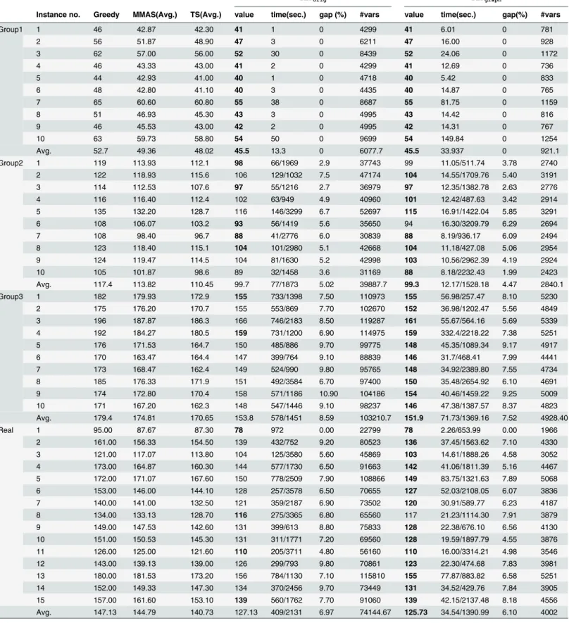
Table 1presents the comparison among the results ofILPgraphand other competitive
sixth column is the time in second, presented as X/Y format only when the solver has been unable to find the optimal solution in 3600 cpu seconds; otherwise it is shown as a single value format reporting the time to get the optimal solution. The seventh column report the relative gap, where gap is defined as the difference between the value of the best valid solution (primal bound) and the lower bound (dual bound) of the problem. The relative gap is formulated as
j(upperbound−lowerbound)/min(jupperboundj,jlowerboundj)j. The eighth column is the number of variables in the formulation for the instance. The last four columns report the result of our formulation,ILPgraph. The columns here reports the same information as the fifth to
eighth columns. The best result for an instance is boldfaced.
FromTable 1, it is easily verified thatILPgraphprovides much better common partition
size than other approaches. Out of 45 instances, it provides equal or better partition size than ILPorigin 42 cases, amongst which 23 are strictly better. The improvement is not only in the
solution size but also in computational time. Except for Group1,ILPgraphhas been able to
achieve improved solution in significantly less time thanILPorig. The number of variables are
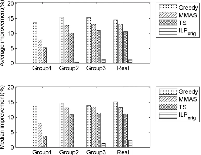
also dramatically reduced inILPgraph.Fig 1, shows the percentage of improvement of
ILP-graphover the other five approaches considered. The significant improvement can be perceived
from the figure.
Table 2reports the average results of Group4 dataset. Here the average of the results of 10 instances for each length group having a particular alphabet size is reported. For example, the first row reports the average results of ten 100-length instances on an alphabet size of 4. The result ofILPorigis collected through personal communication with the author of [14]. It is
notable that for the Group4 dataset,ILPorigwas implemented using GCC 4.7.3 and IBM
ILOG CPLEX V12.1. Moreover, as reported in [14], the corresponding experiments were con-ducted on a cluster of PCs with 2933MHz Intel(R) Xeon(R) 5670 CPUs having 12 nuclei and 32GB RAM. The third to seventh columns report the solution ofILPorigwhile the eighth to
thirteenth columns report the solution ofILPgraph. The columns report the same information
as inTable 1with four exceptions as follows. Firstly, the time when the first valid solution is achieved and the time when the best solution is achieved within the time limit (3600 sec) are presented in two different columns (labelled asftimeandtimerespectively). Secondly, for each formulation, how many among the 10 instances (represented by each row) have been solved optimally is reported in the column named#opt. Finally, the last two columns represent the percentage of improvement in average partition size and the percentage of decrease in the number of variables ofILPgraphoverILPorigrespectively.
Like Group1-Group3 and Real dataset, the results ofTable 2draw the same conclusion. The ILPgraphformulation provides better solutions thanILPorigin almost every aspect.
Numeri-cally,ILPgraphgets equal or better average partition in 28 out of 30 instances of which 12 are
strictly better. The number of instances solved optimally byILPgraphis 172 (out of 300)
which is 12 more than that ofILPorig. The percentage of improvements in the average
solu-tions also proves the superiority ofILPgraph. As it is evident fromTable 2, the improvement
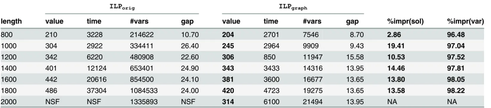
gets more acute with the increase of the string length and the decrease of the alphabet size. This observation is also supported byTable 3that reports the solutions of the two formulations for Group5 dataset. The 7 instances of Group5 were introduced in [14] to test the limit of their for-mulation. Their simulation [14] was conducted in a cluster of PCs with“Intel(R) Xeon(R) CPU 513”CPUs of 4 nuclei of 2000 MHz and 4 Gigabyte of RAM with the time limit of 12 hours. On the other hand, for this dataset, we have enforced 3600 seconds for the first 5 instances and 7200 seconds for the last two.ILPorigcould not achieve a valid solution for the last instance
even within 12 hours whereasILPgraphgot a valid solution in 6100 seconds. From the
Table 1. Comparison for Group1-Group3 and Real dataset.
ILPorig ILPgraph
Instance no. Greedy MMAS(Avg.) TS(Avg.) value time(sec.) gap (%) #vars value time(sec.) gap(%) #vars
Group1 1 46 42.87 42.30 41 1 0 4299 41 6.01 0 781
2 56 51.87 48.90 47 3 0 6211 47 16.00 0 928
3 62 57.00 56.00 52 30 0 8439 52 24.06 0 1172
4 46 43.33 43.00 41 2 0 4299 41 12.69 0 736
5 44 42.93 41.00 40 1 0 4718 40 5.42 0 833
6 48 42.80 41.10 40 3 0 4435 40 14.87 0 765
7 65 60.60 60.80 55 38 0 8687 55 81.75 0 1159
8 51 46.93 45.30 43 3 0 4995 43 14.42 0 816
9 46 45.53 43.00 42 2 0 4995 42 14.31 0 767
10 63 59.73 58.80 54 50 0 9699 54 149.84 0 1254
Avg. 52.7 49.36 48.02 45.5 13.3 0 6077.7 45.5 33.937 0 921.1
Group2 1 119 113.93 112.1 98 66/1969 2.9 37743 99 11.05/511.74 3.78 2740
2 122 118.93 115.6 106 129/1032 7.5 47174 104 14.55/1709.76 5.40 3191
3 114 112.53 107.6 97 55/1216 2.7 36979 97 12.35/1382.78 2.63 2776
4 116 116.40 112.4 102 63/949 4.9 40960 101 12.42/487.63 3.42 2914
5 135 132.20 128.7 116 146/3299 6.7 52697 115 16.91/1422.04 5.85 3291
6 108 106.07 103.2 93 56/1419 5.6 35650 94 16.30/3209.79 6.29 2694
7 108 98.40 96.7 88 41/2776 6.0 30839 88 8.19/936.17 6.09 2494
8 123 118.40 115.1 104 101/2980 5.1 42668 104 11.18/427.08 5.06 2954
9 124 119.47 114.5 104 81/1630 5.2 42998 103 10.56/2962.39 4.19 2924
10 105 101.87 98.6 89 32/1458 3.6 31169 88 8.18/2232.43 1.99 2423
Avg. 117.4 113.82 110.45 99.7 77/1873 5.02 39887.7 99.3 12.17/1528.18 4.47 2840.1
Group3 1 182 179.93 172.9 155 733/1398 7.50 110973 155 56.98/257.47 8.10 5230
2 175 176.20 170.7 155 553/869 7.70 102670 152 36.98/1202.47 5.56 4849
3 196 187.87 186.3 166 746/2183 8.50 119287 161 55.67/564.16 5.69 5339
4 192 184.27 180.5 159 731/1200 6.90 114975 159 332.4/2218.22 7.38 5251
5 176 171.53 164.7 150 485/886 9.70 99775 148 45.35/1089.34 9.17 4917
6 170 163.47 164.4 147 399/764 9.10 88839 146 31.7/468.41 7.99 4441
7 173 168.47 162.4 149 524/990 9.80 95765 148 34.92/2389.80 7.55 4734
8 185 176.33 171.9 151 492/3584 6.70 97400 150 35.48/2654.92 6.10 4691
9 174 172.80 170.4 158 571/1186 10.90 104186 154 40.46/1459.22 9.25 5009
10 171 167.20 162.3 148 547/1446 9.10 98237 146 47.38/1387.57 8.37 4823
Avg. 179.4 174.81 170.65 153.8 578/1451 8.59 103210.7 151.9 71.73/1369.16 7.52 4928.40
Real 1 95.00 87.67 87.30 78 972 0.00 22799 78 2.26/653.99 0.00 1966
2 161.00 156.33 154.50 139 432/752 9.20 80523 136 37.45/1563.62 7.10 4330
3 121.00 117.07 113.80 104 125/3580 5.60 45869 103 14.61/1888.26 4.58 3052
4 173.00 164.87 160.30 144 577/1730 6.50 91663 142 41.06/1811.39 5.16 4467
5 172.00 171.07 167.60 150 778/2509 7.90 108866 149 83.75/1321.63 7.89 5068
6 153.00 146.00 144.10 128 257/3578 6.50 70655 127 52.03/2108.05 6.07 3836
7 140.00 141.00 132.50 121 359/2187 6.90 73502 120 30.91/589.77 6.23 4187
8 134.00 133.13 128.70 116 275/3365 6.80 65560 117 21.23/1114.30 7.91 3879
9 149.00 147.53 142.60 131 399/613 8.80 75833 128 22.38/676.10 6.56 4130
10 151.00 150.53 145.30 131 311/1771 7.20 69560 128 19.59/1897.79 4.55 3876
11 126.00 125.00 121.60 110 205/3711 4.80 56160 110 16.00/3314.21 4.98 3546
12 143.00 139.13 139.00 126 299/793 9.80 70861 123 22.30/474.68 7.83 3981
13 180.00 181.53 173.20 156 784/1130 7.10 115810 155 77.87/883.82 6.58 5251
14 152.00 149.33 147.30 134 370/2456 9.70 73449 131 34.52/429.76 7.84 3905
15 157.00 161.60 153.10 139 560/1762 7.70 91060 139 42.15/2137.48 8.18 4556
Avg. 147.13 144.79 140.73 127.13 409/2131 6.97 74144.67 125.73 34.54/1390.99 6.10 4002
size with less time as the length of the string increases. The number of variables also become intractable forILPorigas the length increases. All of these results speak in favor ofILPgraph.
Finally, to further test the limit of our formulation, i.e.,ILPgraph, we have conducted an
experiment with an instance of length 3000 on the machine with 8GB of RAM. The time limit was set to 12 hours.ILPgraphhas been able to get a valid solution of partition size 642 in 11
hours.
5.4 Running Time
In the previous section, we have shown thatILPgraphprovides much better partition size. In
this section we will explore the running time ofILPgraph. It is clear from Tables1–3that
ILPgraphachieves faster solution in most of the cases even running on a slower processor
Fig 1. Percentage of improvement ofILPgraphover Greedy, MMAS, TS andILPorig.Top: Improvement in average solution. Bottom: Improvement in median solutions.
Table 2. Comparison of average results on Group4 dataset.
ILPorig ILPgraph
length alphabet Size
value ftime time #opt gap #vars value ftime time #opt gap #vars %impr (sol)
%impr (var)
100 4 37.3 0 0 10 0.00 3425.6 37.3 0.17 5.04 10 0.00 649.7 0.00 81.03
12 68.5 0 0 10 0.00 993.3 68.5 0.04 0.05 10 0.00 324.0 0.00 67.38
20 79.8 0 0 10 0.00 622.4 79.8 0.02 0.02 10 0.00 264.2 0.00 57.55
200 4 63.5 3 101 10 0.00 13498.5 63.5 2.67 210.75 10 0.00 1473.8 0.00 89.08
12 119.2 0 0 10 0.00 3824.6 119.2 0.23 0.59 10 0.00 762.8 0.00 80.06
20 146.2 0 0 10 0.00 2301.1 146.2 0.08 0.08 10 0.00 591.6 0.00 74.29
300 4 88.5 21 2358 1 3.20 30398.5 88.6 58.76 1455.52 1 3.23 2412.5 -0.11 92.06
12 165.3 1 3 10 0.00 8478.6 165.3 1.04 17.49 10 0.00 1249.1 0.00 85.27
20 206.7 0 0 10 0.00 5029.6 206.7 0.19 0.23 10 0.00 967.0 0.00 80.77
400 4 115.5 89 2159 0 6.70 53658.5 114.3 28.67 1709.47 0 5.65 3369.8 1.04 93.72
12 208.9 3 47 10 0.00 14887.2 208.9 3.61 73.09 10 0.00 1742.1 0.00 88.30
20 261.5 1 1 10 0.00 8932.0 261.5 0.60 0.73 10 0.00 1366.8 0.00 84.70
500 4 139.3 192 870 0 9.10 84004.2 135.8 43.85 1306.94 0 6.84 4411.8 2.51 94.75
12 249.0 10 328 10 0.00 23173.1 249.0 6.04 500.94 10 0.00 2266.2 0.00 90.22
20 312.2 4 4 10 0.00 13761.0 312.2 1.35 4.08 10 0.00 1803.3 0.00 86.90
600 4 162.2 487 1893 0 9.40 120795.1 159.0 131.19 2018.26 0 7.94 5451.3 1.97 95.49
12 291.0 32 1202 2 0.90 33372.6 290.9 19.28 1703.27 4 0.48 2780.3 0.03 91.67
20 362.3 6 12 10 0.00 19543.8 362.3 3.34 14.61 10 0.00 2253.2 0.00 88.47
700 4 187.7 785 2856 0 10.00 164116.2 182.6 179.51 1475.00 0 7.93 6459.3 2.72 96.06
12 331.0 54 1811 0 1.20 45303.9 330.9 11.83 2404.24 0 0.99 3312.0 0.03 92.69
20 408.9 12 120 10 0.00 26588.5 408.9 5.03 70.57 10 0.00 2729.3 0.00 89.74
800 4 221.6 1442 3432 0 14.70 213956.1 207.7 349.98 1674.61 0 10.40 7555.9 6.27 96.47
12 368.7 123 2460 0 1.60 59026.8 369.5 17.87 1936.50 0 1.71 3871.0 -0.22 93.44
20 456.1 33 669 10 0.00 34451.6 456.1 12.09 489.33 10 0.00 3180.1 0.00 90.77
900 4 266.3 1880 2314 0 22.30 271158.3 227.7 491.91 2315.87 0 10.12 8682.5 14.49 96.80
12 408.5 178 2406 0 2.20 74372.5 407.9 26.34 1936.12 0 1.96 4440.8 0.15 94.03
20 501.5 50 1625 6 0.20 43543.4 501.5 11.44 1311.72 7 0.15 3649.8 0.00 91.62
1000 4 288.7 3253 3739 0 21.80 334125.1 249.2 540.01 1752.42 0 10.49 9825.4 13.68 97.06
12 449.2 306 3147 0 2.90 91955.2 445.4 21.53 1784.16 0 1.89 5017.2 0.85 94.54
20 546.9 89 2182 1 0.50 53736.0 546.7 9.99 1224.10 5 0.29 4106.7 0.04 92.36
doi:10.1371/journal.pone.0130266.t002
Table 3. Comparison result for Group5 dataset.NSF means“No solutions found”.
ILPorig ILPgraph
length value time #vars gap value time #vars gap %impr(sol) %impr(var)
800 210 3228 214622 10.70 204 2701 7546 8.70 2.86 96.48
1000 304 2922 334411 26.40 245 2964 9909 9.43 19.41 97.04
1200 342 6220 480908 22.60 306 850 11947 15.58 10.53 97.52
1400 401 12124 653401 24.90 343 3433 14316 13.95 14.46 97.81
1600 442 20616 854500 24.10 381 3600 16677 13.65 13.80 98.05
1800 486 37304 1084533 24.00 420 4723 19275 13.65 13.58 98.22
2000 NSF NSF 1335893 NSF 314 6100 21494 13.95 NA NA
having lesser memory. This is also true for the first valid solution it provides.Fig 2shows the comparison of the average first valid solution time for three groups based on the alphabet size in Group4 dataset. From this figure it is clear thatILPgraphfinds the first valid solution faster
thanILPorigand the difference in the running time becomes more apparent as the length of
the string increases. Now we concentrate on comparing the running time ofILPgraphwith the
other four approaches. The running times of the two tree search algorithms (referred to as TS1 and TS2) are taken from [15]. The running time of MMAS is taken from [19]. The Greedy algorithm is very fast. It gives the output within few seconds. So, in the analysis, we will assume that the output of Greedy algorithm is readily available even at the beginning of the simulation. We have recorded the primal solution (partition size) of our algorithm periodically. Figs3–6
show the detailed runtime comparison among the algorithms for Group1, Group2, Group3
Fig 2. Average time for the first valid solution found byILPgraphon Group4 data.Top: Alphabet size 4. Middle: Alphabet size 12. Bottom: Alphabet size 20.
Fig 3. Avg. solution Vs. time comparison (Group1).
doi:10.1371/journal.pone.0130266.g003
Fig 4. Avg. solution Vs. time comparison (Group2).
Fig 6. Avg. solution Vs. time comparison (Real).
doi:10.1371/journal.pone.0130266.g006
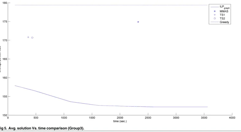
Fig 5. Avg. solution Vs. time comparison (Group3).
and Real datasets respectively. For each group we have shown the average partition size dynamics with respect to time. The three points (“”,“+”,“o”) in each of the figures are the plots of average partition size vs. the average time needed to achieve that partition size for MMAS, TS1 and TS2 approach respectively (data taken from [13], [19]). The dashed line represents the Greedy partition size.
Although the reported time ofILPgraph(inTable 1) is higher than that of Greedy, TS1 and
TS2 approaches in some instances but from the Figs3–6, it can be easily observed that the ILPgraphalgorithm reaches to better solutions much earlier. From the figures it is clear that
ILPgraphis better than Greedy at any stage of time. Even if we stop the algorithm at or earlier
than the average runtime of MMAS, TS1 or TS2, theILPgraphprovides better solutions.
6 Discussion
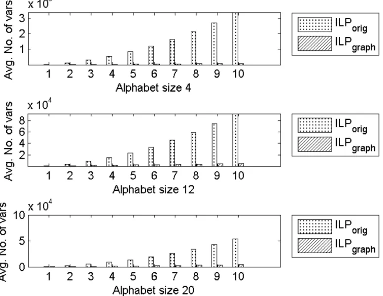
At this point a brief discussion on the number of variables in the two ILP formulations, namely, ILPorigandILPgraph, is in order. InFig 7, we show the comparison of the number of
vari-ables between the two formulations for Group4 dataset. Although both formulations haveO (n2) variables, we observe a significant decrease in the number of variables inILPgraphthan
ILPorig. The average improvement in the number of variables are reported in the last column
of Tables2and3for Group4 and Group5 datasets respectively. For the Group4 dataset the maximum and minimum percentage of decrease in the number of variables are 97.06% and 57.55% with the average improvement of 88.24% while for the Group5 dataset the maximum and minimum are 98.22% and 96.48% with an average of 97.52%.
The drastic improvement in the number of variables forILPgraphand the lack thereof for
ILPorigcan easily be understood by analyzing the variable set of the two formulations.
ILPorigis based oncommon blocks. Acommon block bof two strings (S,T) is defined in [14]
as a triple (t,k1,k2). Heretis a common substring of (S,T) that appeared at positionk1ofS
andk2ofTwhere 0k1,k2n−1.B= {B1,B2,. . .Bm} is the (ordered) set of all common
blocks of (S,T). This set is the variable set ofILPorig. For an example, if (S,T) = (aaagggccc, gggaaaccc), then the number of common blocks would be 42. To find this, first concentrate on a common substring fromSandT, namelyaaa. The common blocks resulting from this com-mon substring are,B= {[a, 0, 3], [a, 0, 4], [a, 0, 5], [a, 1, 3], [a, 1, 4], [a, 1, 5], [a, 2, 3], [a, 2, 4], [a, 2, 5], [aa, 0, 3], [aa, 0, 4], [aa, 1, 3], [aa, 1, 4], [aaa, 0, 3]}. Similar common blocks can be computed for the other two common substrings (gggandccc) too. On the other hand the number of variables inILPgraphdepends on the number of edges in the common substring
graph. Thus, for the above example, if we construct the common substring graph onS, we have 18 edge blocks,E= {[S, 0, 0], [S, 0, 1], [S, 0, 2], [S, 1, 1], [S, 1, 2], [S, 2, 2], [S, 3, 3], [S, 3, 4], [S, 3, 5], [S, 4, 4], [S, 4, 5], [S, 5, 5], [S, 6, 6], [S, 6, 7], [S, 6, 8], [S, 7, 7], [S, 7, 8], [S, 8, 8]}. Thus
ILP-graphreduces the number of variables significantly.
7 Conclusion and Future works
In this paper, we have presented an ILP formulation for the MCSP problem. We have con-ducted extensive experiments and compared the results with the state-of-the-art algorithms in the literature. The results clearly indicate that the ILP formulation is effective and provides excellent results. The observations of Section 5.4 bear important research directions. The research on this field should now be focussed on finding MCSP for larger instances in reason-able time. AsILPgraphprovides better solution faster than the other competitive approaches,
direction could be as follows. So, far MCSP has been studied mostly in the context of opera-tions research. However, it has important applicaopera-tions in genome comparison and rearrange-ment. So, datases from comparative genomics applications could be gathered for further experimental analysis and comparison with relevant algorithms (e.g., [10]) in the field of computational biology.
Supporting Information
S1 Dataset. Group1 dataset.The text file contains 10 instances in pair for Group1 dataset. (TXT)
Fig 7. Comparison of average number of variables betweenILPorigandILPgraphfor Group4 dataset.Top: Alphabet size 4. Middle: Alphabet size 12. Bottom: Alphabet size 20.
S2 Dataset. Group2 dataset.The text file contains 10 instances in pair for Group2 dataset. (TXT)
S3 Dataset. Group3 dataset.The text file contains 10 instances in pair for Group3 dataset. (TXT)
S4 Dataset. Group4 dataset.The compressed folder contains 300 files each containing an instance of lengths from 100 to 1000 separating by alphabet size.
(TGZ)
S5 Dataset. Group5 dataset.The compressed folder contains 7 files each consisting an instance of lengths from 800 to 2000.
(TGZ)
S6 Dataset. Real dataset.The text file contains 10 instances in pair for Real dataset. (TXT)
S7 Dataset. 3000 length instance.The text file contains an instance of length 3000. (TXT)
Acknowledgments
One of the authors, M. Sohel Rahman is currently on a sabbatical leave from Bangladesh Uni-versity of Engineering and Technology (BUET).
Author Contributions
Conceived and designed the experiments: SMF MSR. Performed the experiments: SMF. Ana-lyzed the data: SMF MSR. Contributed reagents/materials/analysis tools: SMF. Wrote the paper: SMF MSR.
References
1. Goldstein A, Kolman P, Zheng J. Minimum Common String Partition Problem: Hardness and Approxi-mations. Electr J Comb. 2005; 12:R#50. Available from:http://www.combinatorics.org/Volume_12/ Abstracts/v12i1r50.html.
2. Chen X, Zheng J, Fu Z, Nan P, Zhong Y, Lonardi S, et al. Assignment of Orthologous Genes via Genome Rearrangement. IEEE/ACM Trans Comput Biol Bioinformatics. 2005 Oct; 2(4):302–315. doi: 10.1109/TCBB.2005.48
3. Chrobak M, Kolman P, Sgall J. The Greedy Algorithm for the Minimum Common String Partition Prob-lem. ACM Trans Algorithms. 2005 Oct; 1(2):350–366. doi:10.1145/1103963.1103971
4. Ferdous SM, Rahman MS. Solving the Minimum Common String Partition Problem with the Help of Ants. In: Tan Y, Shi Y, Mo H, editors. Advances in Swarm Intelligence. vol. 7928 of Lecture Notes in Computer Science. Springer Berlin Heidelberg; 2013. p. 306–313. Available from:http://dx.doi.org/10. 1007/978-3-642-38703-6_36.
5. Dorigo M, Di Caro G, Gambardella LM. Ant Algorithms for Discrete Optimization. Artif Life. 1999 Apr; 5 (2):137–172. doi:10.1162/106454699568728PMID:10633574
6. Watterson GA, Ewens WJ, Hall TE, Morgan A. The chromosome inversion problem. Journal of Theoret-ical Biology. 1982; 99(1):1–7. Available from:http://www.sciencedirect.com/science/article/pii/ 0022519382903848. doi:10.1016/0022-5193(82)90384-8
7. Damaschke P. Minimum Common String Partition Parameterized. In: Crandall K, Lagergren J, editors. Algorithms in Bioinformatics. vol. 5251 of Lecture Notes in Computer Science. Springer Berlin Heidel-berg; 2008. p. 87–98.
9. Jiang H, Zhu B, Zhu D, Zhu H. Minimum Common String Partition Revisited. In: Lee DT, Chen D, Ying S, editors. Frontiers in Algorithmics. vol. 6213 of Lecture Notes in Computer Science. Springer Berlin Heidelberg; 2010. p. 45–52. Available from:http://dx.doi.org/10.1007/978-3-642-14553-7_7.
10. Bulteau L, Fertin G, Komusiewicz C, Rusu I. A Fixed-Parameter Algorithm for Minimum Common String Partition with Few Duplications. In: Darling A, Stoye J, editors. Algorithms in Bioinformatics. vol. 8126 of Lecture Notes in Computer Science. Springer Berlin Heidelberg; 2013. p. 244–258. Available from: http://dx.doi.org/10.1007/978-3-642-40453-5_19.
11. Bulteau L, Komusiewicz C. 8. In: Minimum Common String Partition Parameterized by Partition Size Is Fixed-Parameter Tractable;. p. 102–121. Available from:http://epubs.siam.org/doi/abs/10.1137/1. 9781611973402.8.
12. He D. A Novel Greedy Algorithm for the Minimum Common String Partition Problem. In: Măandoiu I, Zelikovsky A, editors. Bioinformatics Research and Applications. vol. 4463 of Lecture Notes in Com-puter Science. Springer Berlin Heidelberg; 2007. p. 441–452. Available from:http://dx.doi.org/10. 1007/978-3-540-72031-7_40.
13. Blum C, Lozano J, Pinacho Davidson P. Iterative Probabilistic Tree Search for the Minimum Common String Partition Problem. In: Blesa M, Blum C, Voß S, editors. Hybrid Metaheuristics. vol. 8457 of Lec-ture Notes in Computer Science. Springer International Publishing; 2014. p. 145–154. Available from: http://dx.doi.org/10.1007/978-3-319-07644-7_11.
14. Blum C, Lozano JA, Davidson P. Mathematical programming strategies for solving the minimum com-mon string partition problem. European Journal of Operational Research. 2015; 242(3):769–777. Avail-able from:http://www.sciencedirect.com/science/article/pii/S0377221714008716. doi:10.1016/j.ejor. 2014.10.049
15. Achterberg T. SCIP: Solving constraint integer programs. Mathematical Programming Computation. 2009; 1(1):1–41.http://mpc.zib.de/index.php/MPC/article/view/4. doi:10.1007/s12532-008-0001-1
16. Villesen, P. FaBox: An online fasta sequence toolbox; 2007. Available from:http://www.birc.au.dk/ software/fabox.
17. Stothard P. The sequence manipulation suite: JavaScript programs for analyzing and formatting protein and DNA sequences. BioTechniques. 2000 Jun; 28(6). Available from:http://view.ncbi.nlm.nih.gov/ pubmed/10868275.
18. Miltenberger M;. personal communication.
19. Ferdous, SM, Rahman, MS. A MAX-MIN Ant Colony System for Minimum Common String Partition Problem; 2014. Manuscript submitted for publication.