Influence of rainfall observation network on model calibration and application

(1)

www.hydrol-earth-syst-sci.net/12/77/2008/ © Author(s) 2008. This work is licensed under a Creative Commons License.

Hydrology and

Earth System

Sciences

Influence of rainfall observation network on model calibration and

application

A. B´ardossy1and T. Das1,*

1_{Institute of Hydraulic Engineering, Universitaet Stuttgart, 70569 Stuttgart, Germany} *_{now at: Scripps Institution of Oceanography, University of California, San Diego}

Received: 13 November 2006 – Published in Hydrol. Earth Syst. Sci. Discuss.: 11 December 2006 Revised: 26 October 2007 – Accepted: 10 December 2007 – Published: 25 January 2008

Abstract. The objective in this study is to investigate the influence of the spatial resolution of the rainfall input on the model calibration and application. The analysis is car-ried out by varying the distribution of the raingauge network. A meso-scale catchment located in southwest Germany has been selected for this study. First, the semi-distributed HBV model is calibrated with the precipitation interpolated from the available observed rainfall of the different raingauge net-works. An automatic calibration method based on the com-binatorial optimization algorithm simulated annealing is ap-plied. The performance of the hydrological model is ana-lyzed as a function of the raingauge density. Secondly, the calibrated model is validated using interpolated precipitation from the same raingauge density used for the calibration as well as interpolated precipitation based on networks of re-duced and increased raingauge density. Lastly, the effect of missing rainfall data is investigated by using a multiple lin-ear regression approach for filling in the missing measure-ments. The model, calibrated with the complete set of ob-served data, is then run in the validation period using the above described precipitation field. The simulated hydro-graphs obtained in the above described three sets of exper-iments are analyzed through the comparisons of the com-puted Nash-Sutcliffe coefficient and several goodness-of-fit indexes. The results show that the model using different rain-gauge networks might need re-calibration of the model pa-rameters, specifically model calibrated on relatively sparse precipitation information might perform well on dense cipitation information while model calibrated on dense pre-cipitation information fails on sparse prepre-cipitation informa-tion. Also, the model calibrated with the complete set of ob-served precipitation and run with incomplete obob-served data associated with the data estimated using multiple linear re-gressions, at the locations treated as missing measurements, performs well.

Correspondence to:T. Das

(tadas@ucsd.edu)

1 Introduction

Precipitation data is one of the most important inputs re-quired in hydrological modeling and forecasting. In a rainfall-runoff model, accurate knowledge of precipitation is very essential for accurately estimating discharge. This is due to that fact that representation of precipitation is impor-tant in determining surface hydrological processes (Syed et al., 2003; Zehe et al., 2005). Beven (2001) noted that no model, however well founded in physical theory or empiri-cally justified by past performance, will be able to produce accurate hydrograph predictions if the inputs to the model do not characterize the precipitation inputs. Precipitation is governed by complicated physical processes which are inher-ently nonlinear and extremely sensitive (B´ardossy and Plate, 1992). Precipitation is often significantly variable in space and time within a catchment (Krajewski et al., 2003). Singh (1997) provides detailed hydrological literature on the effect of spatial and temporal variability in hydrological factors on the stream flow hydrograph. Wilson et al. (1979) indicated that the spatial distribution and the accuracy of the rainfall input to a rainfall-runoff model influence considerably the volume of storm runoff, peak runoff and time-to-peak. Sun et al. (2002) demonstrated that errors in storm-runoff esti-mation are directly related to spatial data distribution and the representation of spatial conditions across a catchment. They found that the accuracy of storm-runoff prediction depends very much on the extent of spatial rainfall variability. How-ever, Booij (2002) showed that the effect of the model resolu-tion on extreme river discharge is much higher compared to the effect of the input resolution. Bormann (2006) indicated that high quality simulation results require high quality input data, but not necessarily always highly resolved data.

(2)

of earlier studies investigated the influence of the density of the raingauge network on the simulated discharge, with both real and synthetic precipitation and discharge data sets (Krajewski et al., 1991; Peters-Lidard and Wood, 1994; Seed and Austin, 1990; Duncan et al., 1993; St-Hilarie et al., 2003). Michaud and Sorooshian (1994) observed that in-adequate raingauge densities in the case of the sparse net-work produced significant errors in the simulated peaks in a midsized semi-arid catchment. They also found consider-able consistent reductions in the simulated peaks due to the spatial averaging of rainfall over certain spatial resolution. Many researchers have reported the effect of raingauge net-work degradation on the simulated hydrographs (e.g., Brath et al., 2004; Dong et al., 2005). More recently, Anctil et al. (2006) showed that model performance reduces rapidly when the mean areal rainfall is computed using a number of raingauges less than a certain number. They also ob-served that some raingauge network combinations provide better forecasts than when all available raingauges were used to compute areal rainfall. Nevertheless, inadequate represen-tation of spatial variability of precipirepresen-tation in modeling can be partially responsible for modeling errors. This may also lead to the problem in parameter estimation of a conceptual model. Chaubey et al. (1999) found large uncertainty in esti-mated model parameters when detailed variations in the input rainfall were not taken into account. Oudin et al. (2006) ob-served that random errors in rainfall input considerably affect model performance and parameter values, although, model results were nearly insensitive to random errors in potential evapotranspiration input. They also indicated that the sensi-tivity of a rainfall-runoff model to input errors might depend partially on the model structure itself. Chaplot et al. (2005) investigated the effect of the accuracy of spatial rainfall infor-mation on the modeling of water, sediment, and NO3-N loads

for two medium sized catchments under a range of climates, surface areas and environmental conditions. They observed that at both catchments, runoff and nitrogen fluxes are var-ied only slightly with decreasing gauge concentration. They argued that model performance is only slightly affected by data errors because they are able to adjust their parameters in order to compensate for input errors within a reasonable range.

Therefore, it may be of interest to investigate the results of the simulations obtained with the rainfall input when the model is parameterized according to a different type of input data. In fact, it is, frequently the case that a raingauge net-work changes due to an addition or subtraction of raingauges. The raingauge network can be strengthened by the addition of new instruments or by using weather radar, so that a more detailed representation of rainfall is allowed, but for calibra-tion purposes, past observacalibra-tions are available only over the original, less numerous measuring points. Conversely, in the case of an operational flood forecasting system, the oppo-site situation may occur. In the flood forecasting system, the rainfall-runoff model is usually calibrated using all the

avail-able flood events and precipitation data. However, during the operational forecasting time, the precipitation data from all past observation stations may not be available due to a mal-functioning of a few of the observations in the network or the observation data may not be available online. In such cases, it is important to understand if the parameters calibrated using the rainfall coming from one type of network have the abil-ity to represent the phenomena governing the rainfall-runoff process with the input provided by the different configuration of the raingauge network.

Therefore, the aim of this paper is to investigate the influ-ence of rainfall observation networks on model calibration and application. A method based on the combinatorial op-timization algorithm simulated annealing (Aarts and Korst, 1989) is used to identify a uniform set of locations for a par-ticular number of raingauges. First, the semi-distributed con-ceptual rainfall-runoff model HBV is used to investigate the effect of the number of raingauges and their locations on the sensitivity of the hydrological model results. The hydrolog-ical modeling performances of the networks are being ana-lyzed through the comparison of Nash-Sutcliffe coefficient and other goodness-of-fit indices. Secondly, the influence of the rainfall observation network on model calibration and ap-plication is examined. This study seeks to determine whether the parameters calibrated using the rainfall coming from one type of network have the ability to represent the phenom-ena governing the rainfall-runoff process with the input pro-vided by a different configuration of the raingauge network. The model is calibrated using precipitation interpolated from different raingauge networks. The calibrated model is then run for the validation period using the precipitation obtained from the raingauge network, which was not used for the cali-bration. Lastly, the simulation experiments are being carried out to analyze the reliability of supplementing missing pre-cipitation measurements used for the calibration with data estimated using a multiple linear regression and running the model using that precipitation combined with available ob-served precipitation.

2 The study area and data

The upper Neckar catchment, located in southwest Germany, was selected as test catchment. The study area covers an area of approximately 4000 km2_{. The study catchment area}

was divided into thirteen subcatchments depending on the available discharge gauges (Fig. 1).

(3)

12

11 13

10

7 9 8 6 3

4 5

2

1

Fig. 1. Study area: Upper Neckar catchment showing different subcatchments and discharge gauges (Upper-right: location of the study domain in the state of Baden-W¨urttemberg in southwest Ger-many).

in this study were derived from different sources: (1) Dig-ital Elevation Model with a spatial resolution of 50 m×50 m; (2) a digitized soil map of the state of Baden-W¨urttemberg at the scale 1:200 000 and (3) Land use map (LANDSAT satellite image for the year 1993) with a spatial resolution of 30 m×30 m. Daily discharge data from 13 gauging sta-tions was used for model evaluation. All data was provided by the State Institute for Environmental Protection Baden-W¨urttemberg (LUBW). The daily precipitation total, daily maximum and minimum temperature data distributed in and around the study catchment were acquired from the German Weather Service (DWD). The climate of the study area is characterized by warm-to-hot summers with generally mild winters. The coldest and hottest months in the study area are January and July respectively. The daily mean air tempera-ture in January is about−0.8◦C and in July is about 17◦C according to the daily mean temperature records available for the period from 1961 to 1990. The annual variation of precipitation in the study area shows a multi-modal distribu-tion. June and October are the wettest and driest months, with monthly means of 126 mm and 64 mm respectively, ac-cording to the daily amount of raingauge records available for the period from 1961 to 1990. The mean annual precipi-tation observed during this period is 908 mm. The study area has experienced some land use transitions from crop land or grass land to built-up area or industrial usages in the last sev-eral decades (Samaniego, 2003). The use of land cover infor-mation in the HBV model, applied in this study, is static. We have used land use information from the LANDSAT satellite image for the year 1993. The uncertainty might be intro-duced due to this reason and should be explored, but it was not considered in this study since it was not the primary aim.

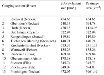
Table 1.Summary of the sizes of the different subcatchments. The table also contains the drainage area of each discharge gauges.

Gauging station (River) Subcatchment Drainage

size [km2] area [km2]

1 Rottweil (Neckar) 454.65 454.65

2 Oberndorf (Neckar) 240.13 694.78

3 Horb (Neckar) 420.18 1114.96

4 Bad Imnau (Eyach) 322.94 322.94

5 Rangendingen (Starzel) 119.89 119.89

6 Tuebingen Blaesibg (Steinlach) 140.21 140.21

7 Kirchentellinsfurt (Neckar) 613.33 2311.33

8 Wannweil (Echaz) 135.26 135.26

9 Riederich (Erms) 169.84 169.84

10 Oberensingen (Aich) 178.18 178.18

11 Suessen (Fils) 345.74 345.73

12 Plochingen (Fils) 349.09 694.83

13 Plochingen (Neckar) 472.05 3961.49

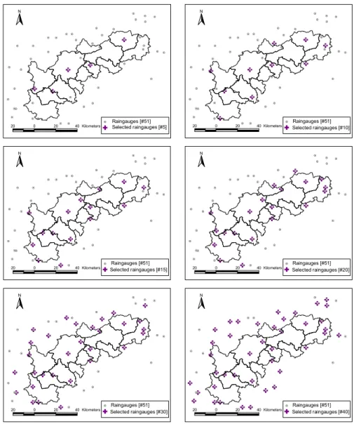
2.1 Raingauge selection method and data preparation The raingauges that have no missing measurements for the period from 1961 to 1990 and are located within or up to 30 km from the study catchment were used as a basis of complete raingauge network. The raingauge networks were selected from the complete network, consisting of 51 rain-gauges, using the combinatorial optimization algorithm sim-ulated annealing (Aarts and Korst, 1989). The main idea be-hind the raingauge selection algorithm is to identify a uni-form set of locations for a particular number of raingauges over the catchment. This means that for number of stations objective functions consisting of the mean distance of the sta-tion to the whole catchment and the minimum distance be-tween the stations were considered. While the first objective was minimized to get internal stations and the second ob-jective was maximized so not to take stations that were very close to each other. The selection algorithm was applied re-peatedly to obtain optimal locations of different number of raingauges. Seven networks consisting of different number of raingauges ranging from 5 to 51 were obtained. Figure 2 shows the spatial distribution of the selected raingauge net-works.

(4)

Ñ Ñ Ñ Ñ _Ñ # Y # Y # Y # Y # Y # Y # Y # Y # Y # Y # Y # Y #

Y Y#

# Y # Y # Y # Y # Y # Y # Y # Y # Y # Y # Y # Y # Y # Y # Y # Y # Y # Y # Y # Y #

Y #Y

# Y # Y # Y # Y # Y # Y #

Y #Y

# Y # Y # Y # Y # Y # Y # Y

Ñ Selected raingauges [#5]

#

Y Raingauges [#51]

20 0 20 40 Kilometers N Ñ Ñ Ñ Ñ Ñ Ñ Ñ Ñ Ñ Ñ # Y # Y # Y # Y # Y # Y # Y # Y # Y # Y # Y # Y #

Y #Y

# Y # Y # Y # Y # Y # Y #

Y #Y

# Y # Y # Y # Y # Y # Y # Y Ñ #

Y Raingauges [#51]

20 0 20 40 Kilometers N

Selected raingauges [#10]

Ñ Ñ Ñ Ñ Ñ Ñ Ñ Ñ Ñ Ñ Ñ Ñ Ñ Ñ Ñ # Y # Y # Y # Y # Y # Y # Y # Y # Y # Y # Y # Y #

Y #Y

Y Y# # Y # Y # Y # Y # Y # Y #

Y #Y

# Y # Y # Y # Y # Y # Y # Y Ñ #

Y Raingauges [#51]

Ñ Ñ Ñ Ñ Ñ Ñ Ñ Ñ Ñ Ñ Ñ Ñ Ñ Ñ Ñ Ñ Ñ Ñ Ñ Ñ # Y # Y # Y # Y # Y # Y # Y # Y # Y # Y # Y # Y #

Y #Y

# Y # Y # Y # Y # Y # Y #

Y #Y

# Y # Y # Y # Y # Y # Y # Y Ñ #

Y Raingauges [#51]

Ñ Ñ Ñ Ñ Ñ Ñ Ñ Ñ Ñ Ñ Ñ Ñ Ñ Ñ Ñ Ñ Ñ Ñ Ñ Ñ Ñ Ñ Ñ Ñ Ñ _Ñ Ñ Ñ Ñ Ñ # Y # Y # Y # Y # Y # Y # Y # Y # Y # Y # Y # Y #

Y #Y

Y Y# # Y # Y # Y # Y # Y # Y #

Y #Y

# Y # Y # Y # Y # Y # Y # Y Ñ #

Y Raingauges [#51]

Ñ Ñ Ñ Ñ Ñ Ñ Ñ Ñ Ñ Ñ Ñ Ñ Ñ Ñ Ñ Ñ Ñ Ñ Ñ Ñ Ñ Ñ Ñ Ñ Ñ Ñ Ñ Ñ Ñ Ñ Ñ Ñ Ñ Ñ Ñ Ñ Ñ Ñ Ñ Ñ # Y # Y # Y # Y # Y # Y # Y # Y # Y # Y # Y # Y #

Y #Y

# Y # Y # Y # Y # Y # Y #

Y #Y

# Y # Y # Y # Y # Y # Y # Y Ñ #

Y Raingauges [#51]

Fig. 2.Spatial distribution of the selected raingauge networks.

uniformly dense over the whole catchment they are more or less uniform for each subcatchment.

Note that the rate of increase of precipitation decreases with increasing elevation. The square root of the topographic elevation was assumed as a good approximation to account for this variation and it was used as the drift variable for pre-cipitation (Hundecha and B´ardossy, 2004). Because the tem-peratures show a fairly constant lapse rate, topographic ele-vation was used as the drift variable for interpolating the tem-perature from the available point measurements. For precip-itation the experimental variogram is calculated for each day when the daily precipitation amount exceeds some threshold values (maximum greater than 10 mm or mean greater than 5 mm). The experimental variogram is then fitted with theo-retical variogram using automatic fitting procedure. The av-erage variogram is used in the remaining days when the daily precipitation amount is low. The average variogram is also

(5)

the period 1961-1990.

mm2day-2 17 - 24 24 - 31 31 - 38 38 - 45 45 - 52 52 - 59 59 - 66 66 - 73 >73 No Data

Fig. 3. Average daily variance (mm2day−2)over each grid of the catchment. The variance is calculated, using the interpolated pre-cipitation computed with the 51 raingagues for the period 1961-1990.

The potential evapotranspiration was computed using the Hargreaves and Samani method (Hargreaves and Samani, 1985) on the same grid used for the interpolation of mete-orological variables.

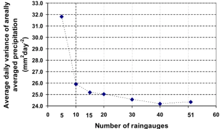
Figure 4 depicts the average daily variance obtained us-ing the averaged areal precipitation over the catchment, com-puted with the selected network densities, for the simulation period (1961–1990). As can be seen that the variability of the interpolated precipitation decreases with the increasing number of raingauges, but there is no change in the variabil-ity beyond a certain number of raingauges. The reason for this is that the contribution of individual stations to the areal average is the higher if less number of stations are used for interpolation. Thus, the interpolation using the smallest num-ber of observations resembles the most variances calculated for each single location.

3 Model and methods

The HBV model is a semi-distributed conceptual model and was originally developed at the Swedish Meteorological and Hydrological Institute (SMHI) (Bergstr¨om and Forsman, 1973). The area to be modeled is divided into a number of subcatchments and each subcatchment is further divided into a number of zones based on elevation, land use or soil type or combinations of them. Snow accumulation and melt, actual soil moisture and runoff generation processes are calculated for each zone using conceptual routines. The snow accumu-lation and melt routine uses the degree-day approach. Ac-tual soil moisture is calculated by considering precipitation and evapotranspiration. Runoff generation is estimated by a non-linear function of actual soil moisture and precipitation. The dynamics of the different flow components at the sub-catchment scale are conceptually represented by two linear reservoirs. The upper reservoir simulates the near surface

24.0 25.0 26.0 27.0 28.0 29.0 30.0 31.0 32.0 33.0

0 10 20 30 40 50 6

Number of raingauges

A

ver

ag

e dai

ly var

ia

nce of

ar

eal

ly

aver

ag

ed p

reci

p

it

a

ti

on

(m

m

2day -2)

0 51 5 15

Fig. 4. Average daily variance (mm2day−2)of areally averaged precipitation vs. number of raingauges. The variance is calculated, using the interpolated precipitation computed with different rain-gague networks for the period 1961–1990.

and interflow in the sub-surface layer, while the lower reser-voir represents the base flow. Both reserreser-voirs are connected in series by a constant percolation rate. Finally, there is a transformation function, consisting of a triangular weighting function with one free parameter, for smoothing the gener-ated flow. The flow is routed from one node to the other of the river network by means of the Muskingum method. Additional description on the HBV model can be found in Lindstr¨om et al. (1997) and Hundecha and B´ardossy (2004). For this study, we considered topographic elevation in defining the zones. This is due to the reason that elevation affects the distribution of the basic meteorological variables such as precipitation and temperatures as well as the rate of evaporation and snow melt and accumulation. Elevation zones were defined using a contour interval of 75 m. The el-evation of the study area varies from about 250 m to around 1000 m, so therefore a maximum of 10 elevation zones were defined in each subcatchment. The mean daily precipitation amount and the mean daily temperature were assigned as in-put to each zone. The meteorological variables for each zone were estimated as the mean of the interpolated values on the regular grids of 1 km2located within a given zone. The po-tential evapotranspiration was also averaged over each zone from the potential evapotranspiration calculated on 1 km2 grids located within a given zone.

3.1 Model calibration and simulations

(6)

of the Nash-Sutcliffe coefficient corresponding to daily and annual time steps was maximized, while a reasonable range was fixed to constrain model parameters. Note that the model calibration and validation were performed using the daily discharges at each subcatchment outlet (total number of sub-catchments is 13). During the calibration, the model parame-ters of the head water subcatchments were optimized before the mixed subcatchments.

The standard split sampling model calibration procedure was followed. The model calibration period runs from 1961 to 1970. The subsequent period up to 1990 was used to val-idate the calibrated model. The interpolated precipitation, based on daily recorded observations, from the different rain-gauge networks was used to simulate the model discharges for the calibration and validation periods. The meteorologi-cal conditions do not differ strongly between the meteorologi-calibration and validation periods for the same raingauge network. 3.2 Simulation comparison statistics

The simulation results obtained using different raingauge networks were compared using the following different statis-tical criteria: the Nash-Sutcliffe coefficient, the relative bias, the peak error and the root mean squared error.

The Nash-Sutcliffe coefficient (R_m2)(Nash and Sutcliffe, 1970) is defined as

R_m2 =1−

N P

i=i

(Qs(ti)−Qo(ti))2

N P

i=1

(Qo(ti)−Qo)2

(1)

whereQo(ti)andQs(ti)are observed and simulated daily

discharge at time step ti respectively and Qo is mean

ob-served daily discharge and N is the total number of time steps.

The relative bias was computed to examine the model per-formance with regard to its ability to maintain the water bal-ance. Additionally the peak error was calculated to check the model’s estimation capacity of the peak flow.

The relative bias (rel. bias) is defined as:

rel.bias=

N P

i=1

(Qs(ti)−Qo(ti))

N P

i=1

Qo(ti)

(2)

Accordingly, the peak error is defined based on the rela-tive difference between the mean annual simulated peak dis-chargeQ_{s (}max)and the mean annual observed peak discharge

Q_o(max):

peak error= ¯

Qs(max)− ¯Qo(max)

¯

Qo(max)

(3) The root mean squared error (RMSE) was also calculated.

Further more, the mean model performance(R_mm2 )is cal-culated using the Nash-Sutcliffe coefficient values obtained at the discharge gauges during the calibration and validation periods.

R_mm2 = 1

L

L X

i=1

[R_m2(calibration)i+Rm2(validation)i]

2 (4)

where R2_m(calibration)i and R2m(validation)i are

Nash-Sutcliffe coefficients during calibration and validation peri-ods for gaugeiandLis the total number of gauges.

Note that higher values ofR_mm2 indicate better mean model performance.

Models are not developed for reproducing known past ob-servations. The purpose is to apply them under different conditions (weather, climate or land use). Therefore model quality should also be measured from this viewpoint. The value of model parameters’ transferability (Tm)is computed

by subtracting the model performance for the validation pe-riod from the model performance obtained in the calibration period.

Tm=max

R2_m(calibration)i−Rm2(validation)i,0

i=1,...,L(5)

A better performance on the validation period could be con-sidered as purely random, thus the difference is limited by zero. Lower values ofTmindicate less loss of the model

per-formance in the validation period and better model parame-ters’ transferability.

Additionally, the mean absolute error and root mean squared error were calculated using the model simulated and observed discharges for each annual maximum flood event.

4 Results and discussion

(7)

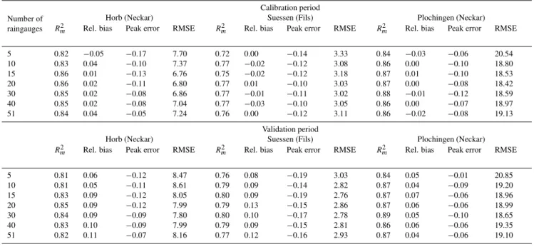
Table 2.Model performance using precipitation interpolated from different numbers of raingauges in the calibration and validation periods.

Number of

Calibration period

raingauges

Horb (Neckar) Suessen (Fils) Plochingen (Neckar)

R2_m Rel. bias Peak error RMSE R_m2 Rel. bias Peak error RMSE R_m2 Rel. bias Peak error RMSE

5 0.82 −0.05 −0.17 7.70 0.72 0.00 −0.14 3.33 0.84 −0.03 −0.06 20.54

10 0.83 0.04 −0.10 7.37 0.77 −0.02 −0.12 3.08 0.86 0.00 −0.10 18.80

15 0.86 0.01 −0.13 6.76 0.75 −0.02 −0.12 3.18 0.87 0.01 −0.10 18.53

20 0.86 0.02 −0.11 6.80 0.77 0.01 −0.10 3.03 0.87 0.00 −0.08 18.42

30 0.85 0.02 −0.08 6.86 0.77 −0.01 −0.11 3.02 0.88 −0.01 −0.12 18.59

40 0.85 0.02 −0.08 7.04 0.77 −0.03 −0.10 3.05 0.86 0.00 −0.07 18.97

51 0.84 0.04 −0.05 7.24 0.76 0.00 −0.12 3.11 0.86 −0.02 −0.08 19.13

Validation period

Horb (Neckar) Suessen (Fils) Plochingen (Neckar)

R2m Rel. bias Peak error RMSE Rm2 Rel. bias Peak error RMSE Rm2 Rel. bias Peak error RMSE

5 0.81 0.06 −0.12 8.47 0.76 0.08 −0.19 3.03 0.84 0.05 −0.01 20.85

10 0.81 0.05 −0.11 8.61 0.79 0.09 −0.14 2.82 0.87 0.04 −0.09 19.20

15 0.83 0.09 −0.12 8.05 0.80 0.09 −0.19 2.76 0.87 0.07 −0.06 18.96

20 0.85 0.09 −0.12 7.99 0.79 0.13 −0.15 2.86 0.87 0.06 −0.06 18.99

30 0.84 0.09 −0.09 7.80 0.80 0.10 −0.17 2.78 0.89 0.05 −0.10 18.65

40 0.83 0.10 −0.09 7.99 0.79 0.09 −0.15 2.81 0.86 0.06 −0.06 19.35

51 0.82 0.11 −0.07 8.16 0.77 0.12 −0.16 2.93 0.87 0.04 −0.06 19.10

0.72 0.73 0.74 0.75 0.76 0.77 0.78 0.79 0.80 0.81

Number of raingauges

N

ash-S

ut

cl

if

fe

co

ef

fi

ci

ent

0.72 0.73 0.74 0.75 0.76 0.77 0.78 0.79 0.80 0.81

Number of raingauges

N

ash-S

ut

cl

if

fe

co

ef

fi

ci

ent

5 10 15 20 30 40 51 5 10 15 20 30 40 51

Fig. 5. Mean Nash-Sutcliffe coefficient calculated on the daily time step resulting from different raingauge networks for the calibration period (left panel) and validation period (right panel).

subcatchment. It seems that the hydrological model used for this study can be well adjusted to the different precip-itation observation densities. A higher spatial model reso-lution might have lead to different results. The number of raingauges within a subcatchment is not necessarily increas-ing with the increase of the total number of stations. For example, for Horb the number of stations within the catch-ment is 5 for the 15 raingauge network and 6 for all denser networks. It can be seen that all stations within the whole catchments are included in all networks consisting of at least 20 raingauges (Fig. 2). The improvement in precipitation in-terpolation seems to be very small, as expected, if raingauges outside the investigation area are also considered. Thus, the subsequent hydrological modeling cannot be improved.

Figure 5 shows the mean Nash-Sutcliffe coefficient calcu-lated on the daily time step for the calibration and validation periods. The mean values were calculated from the Nash-Sutcliffe coefficients obtained at all gauges over the catch-ment. The mean values were calculated to assess the model performance on the calibration and validation periods sepa-rately, and to check the model transferability.

(8)

0.40 0.50 0.60 0.70 0.80 0.90

Winter Spring Summer Fall

Season

N

a

s

h

-S

u

tc

liffe

c

o

e

ffic

ie

n

t

5Raingauges 10Raingauges 15Raingauges 20Raingauges 30Raingauges 40Raingauges

51Raingauges

0.40 0.50 0.60 0.70 0.80 0.90

Winter Spring Summer Fall

Season

N

a

s

h

-S

u

tc

liffe

c

o

e

ffic

ie

n

t

5Raingauges 10Raingauges 15Raingauges 20Raingauges 30Raingauges 40Raingauges 51Raingauges

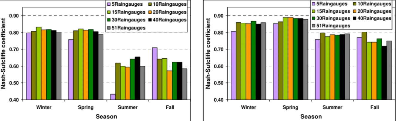
Fig. 6.Seasonal Nash-Sutcliffe coefficients of the daily step using the precipitation interpolated from different number of raingauges during the validation period for the gauges at Suessen (Fils) (left panel) and Plochingen (Neckar) (right panel).

Table 3. Mean model performance and parameters’ transferabil-ity obtained using the precipitation interpolated from different rain-gauge networks. The values are calculated from the Nash Sutcliffe coefficients on daily time step at all the discharge gauges over the catchment.

Number of Mean model Model parameters’ raingauges performance transferability

5 0.74 0.12

10 0.78 0.03

15 0.80 0.04

20 0.80 0.04

30 0.82 0.04

40 0.80 0.05

51 0.80 0.05

Table 3 represents the mean model performance and model parameters’ transferability, calculated using the Eqs. (4) and (5) respectively, corresponding to the different raingauge net-works.

The mean transferability of the model is nearly constant for all precipitation networks except the 5 raingauge case. The reason might be the model resolution lead to an “over fit” for this case. The low transferability values indicate that the model parameters could be reasonably assessed if at least 10 precipitation stations were considered. A least value of mean model performance was observed using the network consisting of 5 raingauges.

There is a considerable difference in the seasonal variabil-ity of precipitation; winter precipitation covers the area more or less uniformly, whereas, convective rainfall in summer leads to high spatial variability. Therefore a seasonal inves-tigation of the model performances is reasonable. Figure 6 shows the seasonal model performance for the Suesen (Fils) and Plochingen (Neckar) gauges.

Figure 6 indicates that the poorest model performance for

all raingauge densities was observed in summer. The results corresponding to the 5 raingauge network are the least con-clusive. All other networks lead to similar performances. This is not surprising as external stations cannot capture local convective events. A better performance could be expected only from a denser internal network.

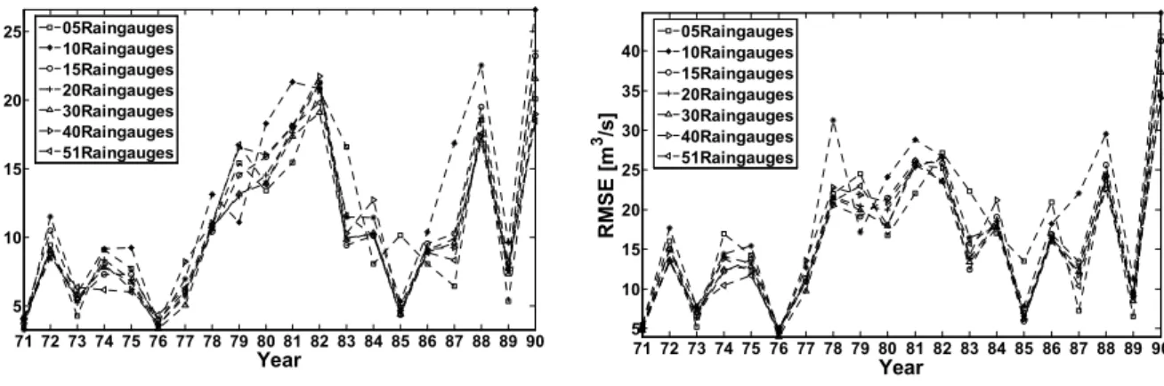
The purpose of modeling is often related to floods; there-fore the model performance for large events is of special in-terest. Subsequently event statistics were calculated for each annual maximum flood event. Figure 7 shows the mean abso-lute error and root mean squared error for the gauge at Horb (Neckar).

The results show a considerable scatter. Differences in the performance are mainly event dependent. On average, the absolute error with respect to the annual maximum dis-charges for the gauge at Horb (Neckar) ranges between 6.9% and 8.4% using the precipitation interpolated from varying raingauge networks. For the 5 and 10 station networks for some events unusually bad performances could be observed. In general the higher densities lead to slightly better model results. The results support the findings corresponding to the mean performance, specifically that improvements will mainly be achieved by using all internal observations.

(9)

71 72 73 74 75 76 77 78 79 80 81 82 83 84 85 86 87 88 89 90 5

10 15 20 25

Year

A

v

e

ra

g

e absolute er

ro

r

[m

3 /s

] 05Raingauges 10Raingauges 15Raingauges 20Raingauges 30Raingauges 40Raingauges 51Raingauges

71 72 73 74 75 76 77 78 79 80 81 82 83 84 85 86 87 88 89 90 5

10 15 20 25 30 35 40

Year

RM

SE

[

m

3 /s]

05Raingauges 10Raingauges 15Raingauges 20Raingauges 30Raingauges 40Raingauges 51Raingauges

Fig. 7.Event statistics for each annual maximum flood event using different raingauge networks during the validation period for the gauge at Horb (Neckar): mean absolute error (left panel) and root mean squared error (right panel).

4.2 Influence of the rainfall observation network on model calibration and application

In the following section, the aim of the simulation exper-iment was to investigate the influence of the spatial reso-lution of the rainfall input on the calibration of a concep-tual model. First, the semi-distributed HBV model was cal-ibrated with the precipitation interpolated from the available observed rainfall of varying raingauge networks. The cali-brated model was then run using the same precipitation used for the calibration as well as interpolated precipitation based on networks of reduced and increased raingauge density.

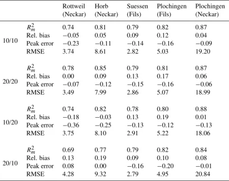
For example, the model was first calibrated using precipi-tation interpolated from 10 and 20 raingauges. The calibrated model using 10 raingauges was then run using precipitation obtained from 20 raingauges for the validation period and vice versa. This experiment is indicated in tables and fig-ures, later on, as follows: 10/10is calibrated with 10 rain-gauges and simulated with 10 rainrain-gauges,20/20is calibrated with 20 raingauges and simulated with 20 raingauges,10/20 is calibrated with 10 raingauges and simulated with 20 rain-gauges and20/10is calibrated with 20 raingauges and simu-lated with 10 raingauges.

The model calibrated using less detailed precipitation (pre-cipitation from 10 raingauges) slightly improves more often when it was run using relatively more detailed precipitation (precipitation from 20 raingauges) (Table 4). On the other hand, the model performance obtained using precipitation from 20 raingauges deteriorated when the same model was run using precipitation obtained from 10 raingauges. Three of the five subcatchments, shown in Table 4, demonstrate the same pattern.

The parameter values, as noted by Brath et al. (2004), may compensate for an incomplete representation of the pre-cipitation field within a reasonable range. Yet, only pro-vided the model parameters were updated by performing re-calibration, for which the new input precipitation was esti-mated from the reduced raingauges network. But there was

0.50 0.55 0.60 0.65 0.70 0.75 0.80 0.85 0.90

Rottweil (Neckar)

Horb (Neckar) Suessen (Fils) Plochingen (Fils)

Plochingen (Neckar)

Na

sh-Sutcliffe coefficie

n

t

10/10 20/20

10/20 20/10

20/20MulRgre

Fig. 8. Nash-Sutcliffe coefficient on the daily time step obtained using different level of precipitation input information for the vali-dation period for selected five gauges.

no such type of compensation for the second case when the calibrated model using 20 raingauges was run using precipi-tation obtained from the 10 raingauge network. This demon-strates the inability of the 10 raingauges to adequately repre-sent the precipitation field for the catchment.

The reason for bad performance with missing data is due to possible systematic differences in precipitation. These can occur due to different elevations or geographical exposition of the whole dataset compared to the remaining stations. A systematic under or overestimation should be avoided.

(10)

Table 4.Model performances using the input precipitation information obtained from different number of raingauges.

Rottweil Horb Suessen Plochingen Plochingen (Neckar) (Neckar) (Fils) (Fils) (Neckar)

10/10

R_m2 0.74 0.81 0.79 0.82 0.87

Rel. bias −0.05 0.05 0.09 0.12 0.04 Peak error −0.23 −0.11 −0.14 −0.16 −0.09

RMSE 3.74 8.61 2.82 5.03 19.20

20/20

R_m2 0.78 0.85 0.79 0.81 0.87

Rel. bias 0.00 0.09 0.13 0.17 0.06

Peak error −0.07 −0.12 −0.15 −0.16 −0.06

RMSE 3.49 7.99 2.86 5.07 18.99

10/20

R_m2 0.74 0.82 0.78 0.80 0.88

Rel. bias −0.18 −0.03 0.13 0.19 0.01 Peak error −0.36 −0.25 −0.13 −0.12 −0.13

RMSE 3.75 8.10 2.91 5.22 18.06

20/10

R_m2 0.69 0.77 0.79 0.82 0.84

Rel. bias 0.13 0.19 0.09 0.10 0.08

Peak error 0.08 0.00 −0.16 −0.20 −0.01

RMSE 4.28 9.32 2.79 4.95 20.84

10/10:calibrated with 10 raingauges and simulated with 10 raingauges;20/20: calibrated with 20 raingauges and simulated with 20 rain-gauges;10/20:calibrated with 10 raingauges and simulated with 20 raingauges and20/10:calibrated with 20 raingauges and simulated with 10 raingauges.

values estimated for the missing stations as uncertain data. The model, calibrated with the precipitation data obtained from 20 raingauges, was then run in the validation period us-ing the precipitation field above described.

Figure 8 shows the model performance for selected five gauges during the validation period using the different level of input precipitation information. The data shown in Ta-ble 4 is partly used to prepare Fig. 8 for easier comparison. In the following tables and figures20/20MulRgreindicates model calibrated with 20 raingauges and simulated with 20 raingauges (rainfall estimated at 10 locations considered as missing measurements). The results from five gauges are shown as they are representative and also these gauges are wide spread in upstream and downstream over the catchment. The model performed well when it was calibrated using precipitation from 20 raingauges and was run with an incom-plete observed data set combined with data generated using the multiple linear regression technique at the locations of the remaining 10 raingauges (Fig. 8). The reason for this is that systematic differences of the rainfall fields are removed by the multiple linear regressions. The similar results are also observed in other subcatchments (not shown).

The performance for flood events was also investigated. Figure 9 depicts the mean absolute error and root mean squared error for the gauge at Rottweil (Neckar).

On average, the absolute error with respect to the an-nual maximum discharges for the gauge at Rottweil (Neckar)

ranges between 6.8% and 8.2%. The highest error was ob-served when the calibrated model using 20 raingauges was run using 10 raingauges. The error reduced to 6.9% when the calibrated model using 20 raingauges was run using 20 raingauges, however, with 10 raingauges of precipitation data estimated using the multiple linear regression technique and the remaining 10 from the observed data. This analysis also supports that the missing measurements can and should be supplemented using a data filling algorithm (in our case mul-tiple linear regression) if additional precipitation information was used for model calibration.

(11)

71 72 73 74 75 76 77 78 79 80 81 82 83 84 85 86 87 88 89 90 2

3 4 5 6 7 8 9 10

Year

A

ve

rag

e

ab

so

lu

te

e

rr

o

r [

m

3 /s]

10/10 10/20 20/20 20/10 20/20MulRgre

71 72 73 74 75 76 77 78 79 80 81 82 83 84 85 86 87 88 89 90 4

6 8 10 12 14 16 18

Year

RMS

E

[m

3 /s

]

10/10 10/20 20/20 20/10 20/20MulRgre

Fig. 9. Event statistics for each annual maximum flood event during the validation period using precipitation obtained from different raingauge networks and estimated precipitation for the gauge at Rottweil (Neckar): mean absolute error (left panel) and root mean squared error (right panel).

Table 5. Nash-Sutcliffe coefficients at 7 days and 30 days time step obtained using different level of precipitation input information for selected five gauges for the validation period.

Gauge Number of raingauges Nash-Sutcliffe coefficient 7 days time

step

30 days time step

Rottweil (Neckar) 20/10 0.76 0.82

20/20MulRgre 0.86 0.90

Horb (Neckar) 20/10 0.80 0.82

20/20MulRgre 0.89 0.91

Suessen (Fils) 20/10 0.82 0.80

20/20MulRgre 0.82 0.80

Plochingen (Fils) 20/10 0.85 0.83

20/20MulRgre 0.85 0.82

Plochingen (Neckar) 20/10 0.88 0.90

20/20MulRgre 0.90 0.92

20/10:calibrated with 20 raingauges and simulated with 10 raingauges and20/20MulRgreindicates model calibrated with 20 raingauges and simulated with 20 raingauges (rainfall estimated at 10 locations considered as missing measurements) (see text).

5 Conclusions

In this paper attempts have been made to investigate the in-fluence of the spatial representation of the precipitation input, interpolated from different raingauge density, on the calibra-tion and applicacalibra-tion of the semi-distributed HBV model. The precipitation input was interpolated using the external drift kriging method from the point measurements of the selected raingauge networks. The performance of the HBV model was assessed using different model performance evaluation criteria for the calibration and validation periods.

A number of simulation experiments were carried out in accordance to the study objective. A first set of

(12)

model resolution can lead to a higher sensitivity on precip-itation observation density. The influence of raingauge den-sity in other regions might be very different depending on the rainfall type (convective or advective), seasonality of precip-itation, importance of snow accumulation and melt, topog-raphy and land use. The more the hydrological processes are complicated the more precipitation observations might be necessary. Temporal variability is influencing the hydro-graph considerably. However, this was not the main interest of this paper - we tried to concentrate on the spatial aspect. A combined space-time investigation would of course be of great interest, which, is beyond the scope of this paper.

A second set of analysis considered the model calibration using precipitation interpolated from one type of raingauge network and was run using precipitation interpolated from another type of raingauge network. The analysis indicated that models using different raingauge networks might need their parameters recalibrated. Specifically, the HBV cali-brated with dense precipitation information fails when run with relatively sparse precipitation information. However, the HBV model calibrated with sparse precipitation informa-tion can perform well when run with dense precipitainforma-tion in-formation.

A third set of experiments analyzed the reliability of sup-plementing missing precipitation measurements used for the calibration with data estimated using a multiple linear re-gression technique, and running the model using that pre-cipitation combined with observed prepre-cipitation. The results showed that the model performs well when it was calibrated with a complete set of observed precipitation and run with an incomplete observed data set combined with estimated data instead of running the calibrated model using incomplete ob-served data only. This result offers an encouraging perspec-tive for the implementation of such a procedure for an oper-ational flood forecasting system. Further research is needed in this direction to prove the practical applicability.

Acknowledgements. The work described in this paper is supported to TD by a scholarship program initiated by the German Federal Ministry of Education and Research (BMBF) and coordinated by its International Bureau (IB) under the program of the International Postgraduate Studies in Water Technologies (IPSWaT). Its contents are solely the responsibility of the authors and do not necessarily represent the official position or policy of the German Federal Ministry of Education and Research. The authors are grateful for the constructive comments of A. Montanari and other two anonymous referees. The helpful comments of H. Bormann, editor of this paper, are gratefully acknowledged.

Edited by: H. Bormann

References

Aarts, E. and Korst, J.: Simulated Annealing and Boltzmann Ma-chines A Stochastic Approach to Combinatorial Optimization and Neural Computing, John Wiley & Sons, Inc., Chichester, 1989.

Ahmed, S. and de Marsily, G.: Comparison of geostatistical meth-ods for estimating transmissivity using data on transmissivity and specific capacity, Water Resour. Res., 23(9), 1717–1737, 1987. Anctil, F., Lauzon, N., Andreassian, V., Oudin, L., and Perrin,

C.: Improvement of rainfall-runoff forecasts through mean areal rainfall optimization, J. Hydrol., 328, 717–725, 2006.

B´ardossy, A. and Plate, E.: Space-Time Model for Daily Rain-fall using Atmospheric Circulation Patterns, Water Resour. Res., 28(5), 1247–1259, 1992.

Bergstr¨om, S. and Forsman, A.: Development of a conceptual de-terministic rainfall-runoff model, Nordic Hydrol., 4, 174–170, 1973.

Beven, K. J.: Rainfall-Runoff Modelling: The Primer, John Wiley and Sons, Chichester, 2001.

Booij, M. J.: Modelling the effects of spatial and temporal reso-lution of rainfall and basin model on extreme river discharge, Hydrol. Sci. J., 47(2), 307–320, 2002.

Bormann, H.: Impact of spatial data resolution on simulated catch-ment water balances and model performance of the multi-scale TOPLATS model, Hydrol. Earth Syst. Sci., 10, 165–179, 2006, http://www.hydrol-earth-syst-sci.net/10/165/2006/.

Brath, A., Montanari, A., and Toth, E.: Analysis of the effects of different scenarios of historical data availability on the cali-bration of a spatially-distributed hydrological model, J. Hydrol., 291, 232–253, 2004.

Chaplot, V., Saleh, A., and Jaynes, D. B.: Effect of the accuracy of spatial rainfall information on the modeling of water, sediment, and NO₃-N loads at the watershed level, J. Hydrol., 312, 223– 234, 2005.

Chaubey, I., Hann, C. T., Grunwald, S., and Salisbury, J. M.: Un-certainty in the models parameters due to spatial variability of rainfall, J. Hydrol., 220, 46–61, 1999.

Dong, X., Dohmen-Janssen, C. M., and Booij, M. J.: Appropriate Spatial Sampling of Rainfall for Flow Simulation, Hydrol. Sci. J., 50(2), 279–297, 2005.

Duncan, M. R., Austin, B., Fabry, F., and Austin, G. L.: The effect of gauge sampling density on the accuracy of streamflow predic-tion for rural catchments, J. Hydrol., 142, 445–476, 1993. Hargreaves, G. H. and Samani Z. A.: Reference crop

evapotranspi-ration from temperature, Appl. Engr. Agric., 1, 96–99, 1985. Hundecha, Y. and B´ardossy, A.: Modeling of the effect of land use

changes on the runoff generation of a river basin through pa-rameter regionalization of a watershed model, J. Hydrol., 292, 281–295, 2004.

Kitanidis, P. K.: Introduction to Geostatistics: Applications in Hy-drogeology, Cambridge University Press, 249 pp., 1997. Krajewski, W. F., Lakshimi, V., Georgakakos, K. P., and Jain, S. C.:

A monte carlo study of rainfall sampling effect on a distributed catchment model, Water Resour. Res., 27(1), 119–128, 1991. Krajewski, W. F., Ciach, G. J., and Habib, E.: An analysis of

small-scale rainfall variability in different climatic regimes, Hydrol. Sci. J., 48, 151-162, 2003.

(13)

hydrological model, J. Hydrol., 201, 272–288, 1997.

Michaud, J. D. and Sorooshian, S.: Effect of rainfall-sampling er-rors on simulations of desert flash floods, Water Resour. Res., 30(10), 2765–2776, 1994.

Montgomery, D. C. and Peck, E. A.: Introduction to linear regres-sion analysis, John Wiley and Sons, New York, New York, USA, 1982.

Nash, J. E. and Sutcliffe, J. V.: River flow forecasting through con-ceptual models. Part I. A discussion of principles, J. Hydrol., 10, 282-290, 1970.

Oudin, L., Perrin, C., Mathevet, T., Andreassian, V., and Michel, C.: Impact of biased and randomly corrupted inputs on the efficiency and the parameters of watershed models, J. Hydrol., 320, 62–83, 2006.

Peters-Lidard, C. D. and Wood, E. F.: Estimating storm areal av-erage rainfall intensity in field experiments, Water Resour. Res., 30(7), 2119–2132, 1994.

Samaniego, L.: Hydrological consequences of landuse/land cover and climatic changes in mesoscale catchments, Doctoral Thesis, University of Stuttgart, Germany, 2003.

Seed, A. W. and Austin, G. L.: Sampling Errors for Raingage De-rived Mean Areal Daily and Monthly Rainfall, J. Hydrol., 118, 163–173, 1990.

Singh, V.: Effect of Spatial and Temporal Variability in Rainfall and Watershed Characteristics on Stream flow Hydrograph, Hydrol. Processes, 11, 1649–1669, 1997.

St-Hilarie, A., Ouarda, T. B. M. J., Lachance, M., Bob´ee, B., Gaudet, J., and Gibnac, C.: Assessment of the impact of meteo-rological network density on the estimation of basin precipitation and runoff: a case study, Hydrol. Processes, 17(18), 3561–3580, 2003.

Sun, H., Cornish, P. S., and Daniell, T. M.: Spatial Variability in Hydrologic Modeling using Rainfall-Runoff Model and Digital Elevation Model, J. Hydrol. Eng., 7(6), 404–412, 2002. Syed, K. H., Goodrich, D. C., Myers, D. E., and Sorooshian, S.:

Spatial characteristics of thunderstorm rainfall fields and their relation to runoff, J. Hydrol., 271, 1–21, 2003.

Wilson, C. B., Valdes, J. B., and Rodriguez-Iturbe, I.: On the influ-ence of the spatial distribution of rainfall on storm runoff, Water Resour. Res., 15(2), 321–328, 1979.