Experimental investigation of the predictive capabilities of data driven modeling techniques in hydrology – Part 2: Application

(1)

HESSD

6, 7095–7142, 2009

Data driven modeling – Part 2: Application

A. Elshorbagy et al.

Title Page Abstract Introduction Conclusions References Tables Figures

◭ ◮

Back Close

Full Screen / Esc

Printer-friendly Version Interactive Discussion

Hydrol. Earth Syst. Sci. Discuss., 6, 7095–7142, 2009 www.hydrol-earth-syst-sci-discuss.net/6/7095/2009/ © Author(s) 2009. This work is distributed under the Creative Commons Attribution 3.0 License.

Hydrology and Earth System Sciences Discussions

This discussion paper is/has been under review for the journal Hydrology and Earth System Sciences (HESS). Please refer to the corresponding final paper in HESS if available.

Experimental investigation of the

predictive capabilities of data driven

modeling techniques in hydrology –

Part 2: Application

A. Elshorbagy1, G. Corzo2, S. Srinivasulu1, and D. P. Solomatine2,3

1

Centre for Advanced Numerical Simulation (CANSIM), Department of Civil & Geological Engineering, University of Saskatchewan, S7N 5A9 Saskatoon, SK, Canada

2

Department of Hydroinformatics & Knowledge Management, UNESCO-IHE Institute for Water Education, Delft, The Netherlands

3

Water Resources Section, Delft University of Technology, Delft, The Netherlands

Received: 29 October 2009 – Accepted: 7 November 2009 – Published: 19 November 2009

Correspondence to: A. Elshorbagy ([email protected])

(2)

HESSD

6, 7095–7142, 2009

◭ ◮

Back Close

Full Screen / Esc

Abstract

In this second part of the two-part paper, the data driven modeling (DDM) experiment, presented and explained in the first part, is implemented. Inputs for the five case stud-ies (half-hourly actual evapotranspiration, daily peat soil moisture, daily till soil moisture, and two daily rainfall-runoffdatasets) are identified, either based on previous studies or

5

using the mutual information content. Twelve groups (realizations) were randomly gen-erated from each dataset by randomly sampling without replacement from the original dataset. Neural networks (ANNs), genetic programming (GP), evolutionary polynomial regression (EPR), Support vector machines (SVM), M5 model trees (M5), K nearest neighbors (K-nn), and multiple linear regression (MLR) techniques are implemented

10

and applied to each of the 12 realizations of each case study. The predictive accu-racy and uncertainties of the various techniques are assessed using multiple average overall error measures, scatter plots, frequency distribution of model residuals, and the deterioration rate of prediction performance during the testing phase. Gamma test is used as a guide to assist in selecting the appropriate modeling technique. Unlike the

15

two nonlinear soil moisture case studies, the results of the experiment conducted in this research study show that ANNs were a sub-optimal choice for the actual evapotranspi-ration and the two rainfall-runoff case studies. GP is the most successful technique due to its ability to adapt the model complexity to the modeled data. EPR performance could be close to GP with datasets that are more linear than nonlinear. SVM is

sen-20

sitive to the kernel choice and if appropriately selected, the performance of SVM can improve. M5 performs very well with linear and semi linear data, which cover wide range of hydrological situations. In highly nonlinear case studies, ANNs, K-nn, and GP could be more successful than other modeling techniques. K-nn is also successful in linear situations, and it should not be ignored as a potential modeling technique for

25

(3)

HESSD

6, 7095–7142, 2009

◭ ◮

Back Close

Full Screen / Esc

1 Introduction

The research methodology explained in the first part of this two-companion paper was implemented in the sequence presented earlier. First, inputs of the various models were identified. A mixed approach of input selection was adopted since identification of optimum inputs was not in itself one of the objectives of this study. The two soil moisture

5

datasets (Elshorbagy and Parasuraman, 2008) and a reduced hourly version of the evapotranspiration (AET) dataset (Parasuraman and Elshorbagy, 2008; Parasuraman et al., 2007) were used in earlier studies. This study benefited from the input structure identified in the earlier studies, and sometimes (e.g., the case of the evapotranspiration dataset) enhanced the input structure by considering more inputs identified using the

10

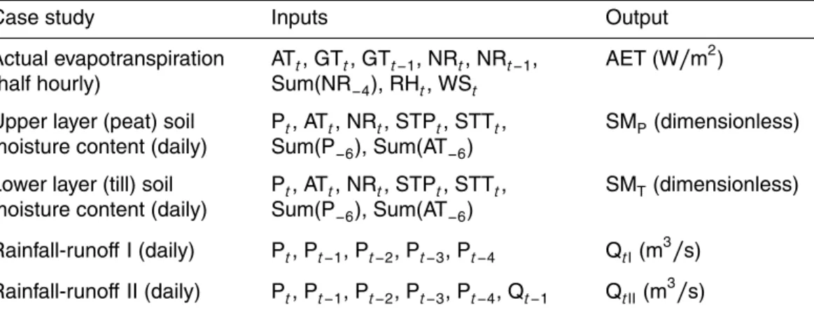
mutual information content. Figure 1 presents the inputs identified for the AET case study using AMI method. For the two rainfall-runoff datasets, the AMI method was used to identify the inputs for predicting the daily runoff(Fig. 2). The inputs-output of the five case studies are presented in Table 1. One should note that in light of the focus of this study, which is the comparative analysis of various data driven techniques, the

15

important criterion is to use the same set of inputs across all adopted models.

After inputs have been identified, each dataset was randomly sampled 100 times; creating 100 realizations of the dataset with three split samples (training, cross-validation, and testing) created from every dataset realization. Figure 3 shows an example of this process for the peat moisture dataset. Similar process was conducted

20

(4)

HESSD

6, 7095–7142, 2009

◭ ◮

Back Close

Full Screen / Esc

2 Model implementation

2.1 Artificial neural networks (ANNs)

The Levenberg-Marquardt algorithm was used for training all neural network models using the MATLAB Neural Networks toolbox. For each realization of the 12 dataset realizations of a case study, the ANN was executed 200 times with 200 different

ran-5

dom weight initializations. The best model of the 200 runs was identified as the best ANN model. The cross validation sub dataset was used to stop the training process. This process was repeated for each of the 12 dataset realization of each case study. Accordingly, 12 ANN models were developed and tested using the corresponding un-seen dataset. In all optimum ANN models, the number of input nodes was equivalent

10

to the number of inputs, and all networks had one output node. The number of hid-den nodes ranged from three to 13, with an average number of seven hidhid-den nodes in single hidden layer ANNs.

2.2 Genetic programming (GP)

Discipulus Software (Francone, 2001) was used to implement the program-based GP

15

to all datasets. GP was applied to the various dataset realizations similar to the way followed with ANNs. The addition, subtraction, multiplication, comparison, conditions, division, and trigonometric operators were allowed. The program size varied from 80– 512 bits, with population size of 500 and generations without improvement up to 300. The probabilities of mutation and crossover were 30% and 50%, respectively. The

20

(5)

HESSD

6, 7095–7142, 2009

◭ ◮

Back Close

Full Screen / Esc

2.3 Evolutionary polynomial regression (EPR)

The EPR Toolbox (Laucelli et al., 2005) was used to implement the static EPR tech-nique to all datasets, following the same experimental steps adopted with the ANNs and the GP techniques. The EPR Toolbox allows for many choices in terms of the polyno-mial types, functions used within the polynopolyno-mial terms, and the number of terms and

5

exponents. In this study, the default number of terms (up to five) was used whereas a comprehensive search among the possible combinations of polynomial types and functions was conducted. Accordingly, 12 non-dominated EPR models were devel-oped and tested on the corresponding testing set of each case study. The EPR type and function developed for each case study are presented in Table 2.

10

2.4 Support vector machine (SVM)

WEKA 3.6.0 Software (Bouckaert et al., 2008) was used in this study to implement the SVM to all datasets, following the same experimental steps adopted with the previous techniques. SVM models with linear, polynomial, and radial basis function (RBF) ker-nels were tested on all datasets. With the exception of the rainfall-runoffII case study,

15

the RBF kernel was found to provide the best predictive performance. In case of the rainfall-runo_ff II case study, both linear and RBF kernels were almost on par. Therefore, SVM with RBF kernel was adopted in this study. The constant C (Elshorbagy et al., 2009) and the kernel parameter γ were optimized from an exponential range of the following values: 0.0313; 0.0625; 0.125; 0.25; 0.50; 1.00; 2.00; 4.00; 8.00; and 16.00.

20

Non-dominated 12 SVM models were developed and tested on the corresponding test-ing set of each case study.

2.5 M5 model trees

WEKA 3.6.0 Software (Bouckaert et al., 2008) was used in this study to implement the M5 model trees to all datasets, following the same experimental steps adopted with the

(6)

HESSD

6, 7095–7142, 2009

◭ ◮

Back Close

Full Screen / Esc

previous techniques. The tree pruning coefficient was optimized during the execution of the models to minimize the average squared error. A range of values from 3–30 was tested in this study. 12 M5 model tree models were developed and tested on the corresponding testing set of each case study.

2.6 K-nearest neighbors (K-nn)

5

WEKA 3.6.0 Software (Bouckaert et al., 2008) was used in this study to implement the K-nn technique to all datasets, following the same experimental steps adopted with the previous techniques. The number of the nearest neighbors was optimized during the execution of the models to minimize the average squared error. A range of values from 1–50 neighbors was tested in this study. Accordingly, 12 K-nn models were developed

10

and tested on the corresponding testing set of each case study. The ranges of the optimum numbers of nearest neighbors for each case study are presented in Table 3.

3 Results and analysis

3.1 Evapotranspiration case study

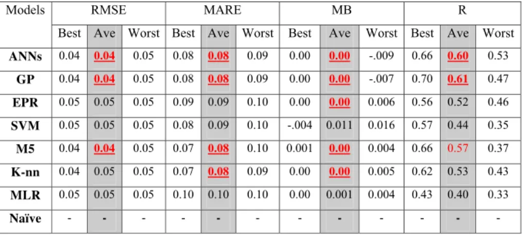
The performance of the various techniques applied to the half-hourly actual

evapotran-15

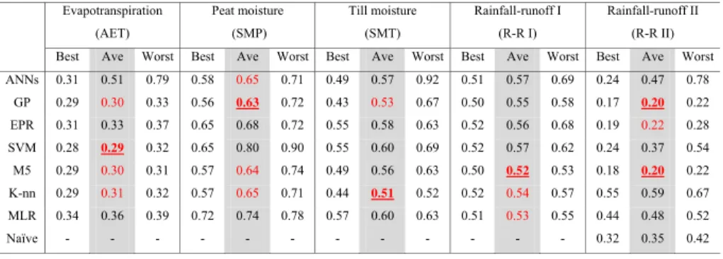
spiration (AET) case study is provided in Table 4. The best, the worst, and the average of the performances of the 12 models of all techniques are shown. It is certainly use-ful to judge techniques based on the range of performances (difference between the best and the worst models), however, if a single value is needed, then one has to rely on the average performance. Table 4 supports the idea that in most cases, it is not

20

(7)

HESSD

6, 7095–7142, 2009

◭ ◮

Back Close

Full Screen / Esc

identified as the best techniques, followed by EPR, in terms of the predictive accuracy. The performance of the ANNs was worse than the linear regression (MLR) technique in this particular case study. This highlights an important fact that the half-hourly AET data were captured reasonably well in a linear relationship considering the provided model inputs. Therefore, a technique that forces highly nonlinear structures on the

5

input-output relationship (ANNs) may not be favorable in all cases. Certainly, the AET data are not strictly linear; that is why local and/or modular linear models (e.g., M5 and K-nn) could be optimum choices.

Since all 12 models of each technique are non-dominated models and represent pos-sible performances of the technique under consideration, the output of all 12 models

10

are integrated in one set and presented in Fig. 4. The figure shows the scatter plots of observed vs. predicted AET data. The scatter around the 45-degree line supports the conclusion made earlier regarding the performances of the various techniques. How-ever, the plots allow to make two additional observations; first, all techniques were less successful in predicting high values. The tips of the data plumes were always below

15

the 45-degree line. This might be an indication that the ideal inputs that can describe all dynamics of the process for this case study have not been optimally identified. The SVM (Fig. 4d) was more successful than other techniques in approaching the high val-ues. The M5 model trees and MLR (Fig. 4e,g) were the least successful in this regard. Table 5 shows the ideal point error (IPE) measure calculated for all techniques. The

20

IPE statistic, integrating all four error measures in one indicator, lends another support to the conclusions made earlier. Except the ANNs, all other techniques have close performances, with the possibility of identifying the SVM, GP, M5, and K-nn; followed by EPR as better techniques than the rest. The utility of the idea of adopting multiple models (12 in this study) based on different random realizations of the datasets to

eval-25

(8)

HESSD

6, 7095–7142, 2009

◭ ◮

Back Close

Full Screen / Esc

much better than the worst EPR model with IPE value of 0.37 (Table 5).

Based on the outputs of the 12 non-dominated models of each technique, the pre-dictive uncertainty of the various techniques can be easily analyzed. The residuals (predicted value minus observed value) of the 12 models were integrated in one set to conduct probabilistic analysis. Frequency curves were constructed for the

residu-5

als of each technique. @RISK Software (Palisade Corporation, 2005) was used to fit the best probability distribution from a selection of more than 15 possible distributions. The best-found probability distributions of the residuals of the various techniques are shown in Fig. 5. The Logistic (α,β) distribution was found to fit the residuals of all mod-eling techniques, with different values of location parameterα and scale parameter β.

10

Ideally, the best technique is the one that has residuals represented by the narrowest, symmetrical, and tallest (has the highest probability value at zero residuals) probabil-ity distribution. Such a distribution implies the smallest level of predictive uncertainty, which could be translated to the highest level of reliability. Figure 5 reveals that, not only in terms of the predictive accuracy, but also the predictive uncertainty SVM is the

15

best, flollowed by GP, K-nn, M5 and EPR. Clearly, the ANN technique leads to the most uncertain results with the widest range of residuals, whereas the MLR is occupying the middle position.

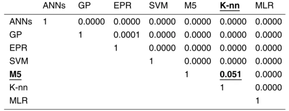
The Kolmogorov-Smirnov (KS) nonparametric test was conducted on the model residuals of all techniques to test the null hypothesis that the model residuals of any

20

two techniques are sampled from the same distribution. The test was conducted at the default significance level of p=0.05. The matrix of the p-values is given as Table 6. With the exception of K-nn and M5 techniques, there is strong statistical evidence that the residuals of the various techniques are stemming from different distributions. There are also no correlations found among the probability distributions of the residuals of the

25

(9)

HESSD

6, 7095–7142, 2009

◭ ◮

Back Close

Full Screen / Esc

3.2 Peat (upper layer) soil moisture case study

The performance of the various techniques applied to the daily soil moisture data of the upper peat layer (SMP) case study is provided in Table 7. Unlike the evapotranspira-tion case study, Table 7 shows that both ANNs and GP techniques can be considered superior to other modeling techniques due to their domination with respect to the four

5

error measures. It has to be noted that in case of soil moisture content, low values of the RMSE and the MARE might be misleading because the entire dataset is limited to a narrow range (0.30–0.55) of values (Table 3, Part I). In this case, the R statistic becomes the most important indicator (Elshorbagy and Parasuraman, 2008). For ex-ample, if an average-all model is constructed just by assuming that the best predictor is

10

the average soil moisture value of all observations in the training dataset, the predicted value will be always 0.442. In this case, the RMSE and the MARE values are 0.05 and 0.10, respectively, but the R statistic value is almost zero; indicating an extremely poor model. Accordingly, ANNs and GP are the best modeling techniques for this case study (producing the R values of 0.60 and 0.61, respectively), followed by the K-nn and

15

the M5 techniques. The MLR is clearly dominated by other techniques, which points to the possibility that the SMP dataset is a highly nonlinear dataset. The authors be-lieve that this is a major reason for the relative success of ANNs in this case study compared to the previous (AET) case study. The moisture storage e_ffect (Elshorbagy and El-Baroudy, 2009; Elshorbagy and Parasuraman, 2008) attributes to the

nonlinear-20

ity of the process. Techniques that can handle highly nonlinear data (ANNs and GP) were quite successful, followed closely by local/modular models (M5 and K-nn). Even though the EPR technique was relatively close to the K-nn and M5, the performance of the SVM technique was the poorest with an R value of 0.44; slightly higher than the MLR.

25

(10)

HESSD

6, 7095–7142, 2009

◭ ◮

Back Close

Full Screen / Esc

that ANNs outperforms other techniques where, at least, the trend of the higher range of peat moisture values was captured better than the other techniques could do. Simi-lar to the AET case study, frequency curves were constructed for the residuals of each technique (Fig. 7). Interestingly, the best-found probability distributions of the residuals of the various techniques di_ffered. The LogLogistic (γ,β,α) probability distribution was

5

found to fit the residuals of SVM and K-nn, and M5 modeling techniques, Logistic (α,

β) for ANNs, Lognormal (µ, σ) for GP, Beta (α1, α2) for EPR and MLR techniques. This reflects the fact that the adopted modeling techniques are di_fferent in the way that they predict the output and minimize the errors, even if their average overall error val-ues are close. The frequency curves reflect the considerable outperformance of the

10

ANNs, K-nn, M5, and SVM over other more uncertain and biased techniques, such as MLR and the EPR techniques. An important observation here is the lower uncertainty of the SVM technique. The small uncertainty of the SVM technique reflected by the probability distribution is a_ffected by the narrow range of residuals and small overall RMSE, however, the SVM models are poor in capturing the trend of the SMP data –

15

this is indicated by the lower R value.

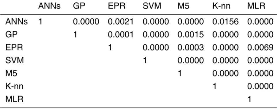
The Kolmogorov-Smirnov nonparametric test was conducted on the model residuals of all techniques to test the null hypothesis that the model residuals of any two tech-niques are sampled from the same distribution. The matrix of the p-values is given in Table 8. There is strong statistical evidence that the residuals of the various techniques

20

are stemming from different populations. There are also no correlations found among the probability distributions of the residuals of the various modeling techniques.

3.3 Till (lower layer) moisture case study

The till moisture case study (SMT) is similar to the previous case study with regard to the small variability in the dataset, and the highly nonlinear response to the climatic

25

(11)

HESSD

6, 7095–7142, 2009

◭ ◮

Back Close

Full Screen / Esc

error measures shown in Table 9 (and in particular the R statistic) reveal that K-nn, GP, and ANNs are better candidates than other modeling techniques based on the same argument mentioned earlier regarding the R statistic. Similar to the previous case study, SVM and MLR techniques were the lowest in the rank with regard to the prediction accuracy. The small variability, combined with the high nonlinearity, of the

5

SMT dataset contributed to the relative success of the K-nn technique in this particular case study. The failure of the MLR is an indicator of the potential utility of the ANNs for modeling the SMT.

Frequency curves were constructed for the residuals of each technique (Fig. 8) to investigate the predictive uncertainty. The graph in this case provides useful and more

10

insightful view of the predictive reliability of the various techniques. The K-nn, GP, ANNs, and the SVM are clearly less uncertain and less skewed than EPR and other linear techniques (M5 and MLR) in this case study. The best-found probability dis-tributions of the residuals of the various techniques di_ffered across techniques. The LogLogistic (γ,β,α) distribution was found to fit the residuals of SVM and K-nn, and

15

ANNs modeling techniques, Logistic (α,β) for GP, Lognormal (µ,σ) for EPR and MLR, and ExtremeValue (a, b) for M5. This reflects the fact that some of the adopted model-ing techniques are really different in the way that they predict the output and minimize the errors, whereas some similarity is identified among the ANNs, K-nn, and SVM techniques. This similarity is only in terms of approaching the optimum solution, and

20

leaving model residuals to be similarly distributed, but not necessarily in the distribution parameters. Similar to the SMP case study, less uncertainty with the use of the SVM is due to model residuals that stay around the mean, and thus, reduce the variability and the average error. This should not be confused with the poor accuracy of capturing trends in the data (low R value in Table 9 and even high IPE value in Table 5).

25

(12)

HESSD

6, 7095–7142, 2009

◭ ◮

Back Close

Full Screen / Esc

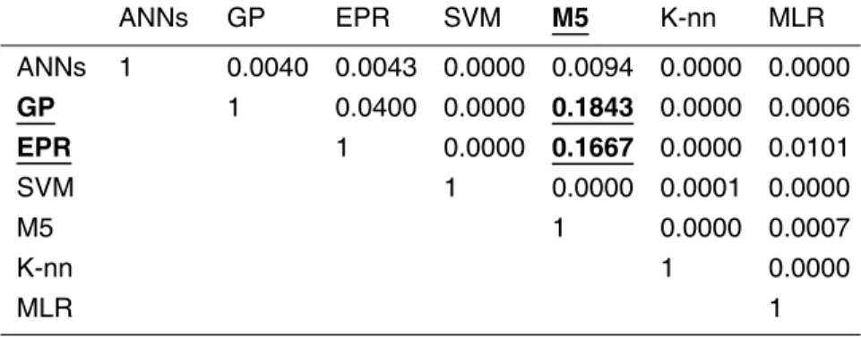
case of the EPR and M5, and also GP and M5. The visual analysis of Fig. 8 confirms the finding regarding EPR and M5; however, M5 and GP are visually different. The reason is that the graph presents the best-fit distributions that should be used to make conclusions regarding the potential of the techniques and their possible performance on untested cases in the future. The KS is a nonparametric test that relies on the

cu-5

mulative frequency of the sample itself. For the rest of the adopted techniques, there is strong statistical evidence that the residuals of the various techniques are stemming from different populations. There are also no correlations found among the probability distributions of the residuals of the various modeling techniques.

3.4 Rainfall-runoffcase study I

10

The performance of the various techniques applied to the daily rainfall-runoffI (R-R I) case study is provided in Table 11. In this case study, the preceding runoffwas not used as an input for the models, therefore, the information content can be considered limited (only rainfall of the current and preceding three days were used). The performances of all techniques were almost on par as shown by close values of average RMSE and

15

R (Table 11) as well as close values of the IPE indicator (Table 5). Nonetheless, one can observe that M5, GP, and MLR were slightly better and less biased (lower MB values) than the other techniques. In a situation like this R-R I case study, where the information content itself is limited; it may not be practical to differentiate among the various modeling techniques. The limiting factor for the prediction accuracy becomes

20

the information content rather than the predictive capability of the various techniques. A linear (e.g., MLR) or a modular linear (M5) technique is sufficient for such dataset.

The best-found probability distributions of the residuals of the various techniques did not di_ffer. The Logistic (α, β) probability distribution, with di_fferent parameter values for each technique, was found to fit the residuals of all modeling techniques. This

25

(13)

HESSD

6, 7095–7142, 2009

◭ ◮

Back Close

Full Screen / Esc

shows almost no practical differences among the various probability distributions, the p-values of the K-S test (Table 12) indicate that there is strong evidence to reject the null hypothesis. Based on the K-S test, the model residuals of the various techniques could represent different distributions. There is no contradiction between the K-S test results and the visual test because a slight shift on the graph might be translated to

5

a statistically significant difference.

3.5 Rainfall-runo_ffcase study II

This rainfall-runoffII (R-R II) case study is the same as the previous R-R I dataset with one di_fference; that is the preceding runo_ff was used as an additional input. In such a strongly autocorrelated series as the daily runoff, providing the preceding runoffas

10

an input to predict the current runoff make strong information content at the disposal of the predictive models. Even though the MLR technique may not be suitable for this case study because one of the inputs (preceding runoff) is autocorrelated, it is used to show how much information can be a captured by a global linear model. In addition to this, a na¨_ıve model for predicting the daily runo_ff was developed just by

15

using the preceding runoffvalue as an estimate of the current runoff. The performance of the various techniques applied to the daily R-R II case study is provided in Table 13. GP, M5, and EPR, followed by the MLR, techniques are better choices than the other techniques for this case studies. They provide the lowest RMSE, MARE, MB, and the highest R values. The IPE indicator in Table 5 also mostly supports this finding.

20

Expectedly, the presence of the preceding runo_ffas an input in this case study makes the input-output relationship more globally linear than nonlinear. The superiority of the MLR over the ANNs supports this idea. Instance-based leaning techniques that use simple average of the nearest neighbors (K-nn) may not be a good choice. K-nn found almost most of the information within a range of very small number of neighbors

25

(14)

HESSD

6, 7095–7142, 2009

◭ ◮

Back Close

Full Screen / Esc

Figure 10 shows the scatter plots of observed vs. predicted runoffII data. The scat-ter around the 45-degree line supports the conclusion made earlier regarding the su-periority of the GP, M5, and EPR, and the inferiority of K-nn, ANNs, and SVM tech-niques. The success of GP, EPR, and M5 across all ranges of the dataset is noticeable (Fig. 10b,c,e). With the exception of the SVM and na¨_ıve models, the best-found

proba-5

bility distributions of the residuals of the various techniques did not differ. The Logistic (α,β) probability distribution, with different parameter values for each technique, was found to fit the residuals of ANNs, GP, EPR, M5, K-nn, and MLR techniques, whereas Normal (µ,σ) was found to fit the residuals of the SVM and the na¨ıve models. In spite of the similarity in the best-fit distribution, the parameters were completely different

10

even visually (Fig. 11). All modeling techniques produced symmetrical distributions of model residuals, but GP, EPR, and M5 possess the smallest predictive uncertainty. The p-values of the K-S test (Table 14) indicate that there is strong evidence to reject the null hypothesis. Based on the K-S test, the model residuals of the various techniques could represent different distributions.

15

4 Discussion

After evaluating the various data driven modeling (DDM) techniques from both per-spectives of prediction accuracy and uncertainty, one of the means to gain further insight into their modeling capabilities is to compare the performance deterioration in the testing phase to that in the training phase. Less deterioration may indicate a higher

20

level of reliability and less uncertainty about the technique’s performance in future and untested applications. The percent deterioration is calculated for each technique by dividing the di_fference between training and testing performance by the training perfor-mance. A negative percent means that the performance of the technique during the testing phase was better than that during the training phase. Table 15 presents the

25

(15)

HESSD

6, 7095–7142, 2009

◭ ◮

Back Close

Full Screen / Esc

used. A few observations can be noted from Table 15: i) ANNs had the highest level of performance deterioration in all case studies, which is an intricate characteristic of the technique and perhaps any highly nonlinear technique. ANNs seem to go after some individual and local patterns even when training is stopped by cross-validation; ii) simi-lar to ANNs, SVM su_ffered from similar phenomenon in four out of the five case studies.

5

This might be counter intuitive and requires further investigation because a technique that employs the concept of error tolerance and flatness of the approximation function should do better in this regard. Users of SVM are encouraged to study further the ef-fect of the error tolerance and the flatness coefficient C on the technique performance; iii) in highly nonlinear case studies (e.g., peat and till soil moisture), the compromise

10

between improving the prediction accuracy while reducing the deterioration might be difficult. The deterioration of the K-nn technique in both case studies was the high-est, while performing relatively better than other techniques in terms of the prediction accuracy and uncertainty; (iv) EPR, almost similar to MLR, was excellent in its general-ization ability. The deterioration of performance during the testing phase was very small

15

in all case studies; highlighting a great potential of this technique; and v) in most cases GP and M5 model trees were not far from the EPR regarding the performance deteri-oration. Therefore, whenever EPR, GP, and M5 are comparable to other techniques in terms of prediction accuracy and uncertainty, they deserve to be given preference as candidate modeling techniques.

20

One of the fundamental questions of this research study is whether there are real differences among the techniques under consideration with regard to their predictive capabilities. The results and analysis show that serious evaluation of the various tech-niques has to rely on multiple ways, such as the average overall error represented by multiple error measures, scatter plots of the observed vs. predicted outputs,

proba-25

(16)

HESSD

6, 7095–7142, 2009

◭ ◮

Back Close

Full Screen / Esc

scatter plots reveal that the models were not behavioral; i.e., could not capture the trend of the phenomenon at all. On the other hand, the superiority of the ANNs over other techniques on the same dataset was revealed by the scatter plots. The analy-sis presented in the previous section shows that SVM, M5, K-nn, and GP techniques were the best candidates for modeling the evapotranspiration case study. In the peat

5

moisture case study, ANNs, GP, and followed by K-nn, M5, and EPR provided the best performances, whereas ANNs, GP, and K-nn were the best for modeling the till mois-ture dataset. Even though the K-S test show that the difference between the residuals of GP and M5 was insignificant, this should be treated with caution. The test compares the residuals but fail to assess the difference in the R statistic, which is the key indicator

10

in this particular case study. M5 was not successful in this highly nonlinear dataset. For the rainfall-runoff I dataset, all techniques were on par, and perhaps there is no need for a sophisticated nonlinear model. In the last case study (rainfall-runoffII), that has an autoregressive term and hence can be described by less non-linear mappings, GP, M5, and EPR were obviously better than the other techniques.

15

Neural networks could be one of the optimum modeling choices for highly nonlinear case studies (e.g., peat and till soil moisture), but could be completely dominated by other techniques as it was the case for the AET and the rainfall-runoffII case study, depending on the level of linearity in the dataset. M5 is an excellent choice for lin-ear and some nonlinlin-ear dataset; it performed poorly only in the till moisture dataset.

20

EPR, though it was not a top choice except in the rainfall-runo_ffII case study, was never completely dominated by other methods, and sometimes it was among the best techniques. The excellent generalization ability (minimum performance deterioration during the testing phase) of the EPR adds to its potential for hydrological applications. However, in highly nonlinear datasets, EPR was always less successful than GP. GP

25

(17)

HESSD

6, 7095–7142, 2009

◭ ◮

Back Close

Full Screen / Esc

significantly affected by the choice of kernels. In this study, the RBF kernel was chosen based on its performance on the cross validation sample of most case studies (four out of five cases). In the linear rainfall-runoffII case study, when a linear kernel was tested, the prediction accuracy, represented by RMSE, MARE, and R, improved by 20–25%.

Two limitations of this study have to be noted. Firstly, the e_ffect of the model inputs

5

on the predictive capabilities was not investigated. Adding more important inputs, or lack of these, affect the degree of linearity/nonlinearity of the input-output relationship, and thus, the model performance. Such an e_ffect may di_ffer from one technique to the other. Secondly, some capabilities of the various techniques and tools were not, and perhaps cannot be, thoroughly covered. The Discipulus software for GP was run

10

for almost two hours each time. It was observed that allowing from 24–48 h of run could slightly improve the results. The EPR tool allows for multiobjective optimization, rather than just minimizing the squared error, but it was not tried in this study. Also instance-based techniques (K-nn) could be further improved using weighted average or regression of the nearest neighbors. ANNs could be trained using Bayesian

regu-15

larization algorithm (Demuth and Beale, 2001), which could improve the generalization ability. In this study, multiobjective cost functions were avoided as much as possible. However, future research by the authors and/or other researchers could add to this experiment and build on it.

The non-parametric Gamma test (Γ-test) (Chuzhanova et al., 1998; Evans and

20

Jones, 2002; and recently applied in hydrology by Remesan et al., 2008) was con-ducted to gain insight into the predictability and the complexities of the modeled pro-cesses, and possible leads into selection of suitable modeling techniques. TheΓ statis-tic was calculated for every dataset using the original training and cross-validation sub-sets as one integrated subset (all unique points). The V-ratio, gradient, and the M-test

25

were all calculated using the scaled data (zero mean and 0.5 standard deviation). The

(18)

tech-HESSD

6, 7095–7142, 2009

◭ ◮

Back Close

Full Screen / Esc

nique (2302) was already lower than theΓstatistic; indicating that complex nonlinear model (e.g., ANNs) may not be necessary. The low gradient value of 0.041 shows that a noncomplex smooth function can be used for modeling the AET process, whereas the reasonably low V-ratio indicates that there is high predictability in the output vari-able. GP, shown to perform well on all case studies, achieved the lowest error variance.

5

Even though it is lower than the estimated Γ, but when it is divided by the AET vari-ance (Table 1, part I), the ratio is 0.23; similar to the V-ratio.; ii) for the R-R I case study, similar to the AET, there is no need for nonlinear complex model, especially in light of the high V-ratio that indicates low level of predictability. The low level of predictability is attributed to the lack of appropriate inputs, which was rectified in the R-R II case study.

10

All techniques were found to perform on par. The slight superiority of the M5 (ratio of error variance to output variance is 0.44), which is a modular linear technique can be attributed to the fact that it does not produce a smooth function. This is something that the_Γ-test may not capture well; iii) similar conclusions can be made for the R-R II case study. Nonlinear techniques, such as ANNs, will not perform well. The very low V-ratio

15

that indicates very high predictability might be achieved by techniques that can outper-form MLR, yet have the ability to adapt to linear situations. As expected GP, EPR, and M5 performed extremely well in this case; iv) both SMP and SMT case studies, the MLR technique failed to achieve the estimatedΓvalue, and actually produced ratios of error variance to output variance of 1.0 and 0.8, respectively. This finding points to the

20

possibility that more complex nonlinear models are needed. As the results of this study show, in addition to GP, the ANNs and K-nn were relatively more successful in the SMP and SMT case studies. However, it should be noted thatΓ-test relates well to the model performance with regard to the squared error, but in cases where the criterion of performance is the R statistic, the test may not be the optimum tool; v) the M-test

25

(19)

HESSD

6, 7095–7142, 2009

◭ ◮

Back Close

Full Screen / Esc

training datasets exceeded the M-test.

The Γ-test may assist in the selection of the appropriate modeling techniques by applying first multiple linear regression models and evaluating the residuals against theΓ-test values. Decision can be made regarding the need for a complex nonlinear technique. If there is a need for such technique, then ANNs and K-nn (in addition to GP,

5

for example) should be seriously considered. If it is concluded that complex nonlinear techniques are not needed, then improvement of results can be sought using GP, EPR, and M5. When complex nonlinear techniques are not needed, and the predictability is low (i.e., high V-ratio) significant improvement may not be at all possible.

5 Conclusions

10

Neural networks (ANNs) that have hidden nodes with nonlinear transfer functions may impose on the data a model with complexity level that is higher than that needed by many hydrological data. The results of the experiment conducted in this research study show that ANNs were a sub-optimal choice for the actual evapotranspiration (AET) and the two rainfall-runoff case studies. In the highly nonlinear case studies (peat and

15

till soil moisture), ANN models were the most successful ones. In general, genetic programming (GP) was the most successful technique due to its ability to adapt the model complexity to the modeled data. Evolutionary polynomial regression (EPR) per-formance could be close to the GP with datasets that are more linear than nonlinear. Support vector machines (SVM) are sensitive to the kernel choice and if appropriately

20

selected, the performance of SVM can improve. M5 model trees performs very well with linear and semi linear data, which cover wide range of hydrological situations. In highly nonlinear case studies, ANNs, K nearest neighbors (K-nn), and GP could be more successful than other modeling techniques. K-nn was also successful in linear situations, and it deserves more attention as a potential modeling technique for

hydro-25

logical applications.

(20)

(realiza-HESSD

6, 7095–7142, 2009

◭ ◮

Back Close

Full Screen / Esc

tions) of each dataset should be randomly generated, by sampling without replace-ment, and should be divided into three split samples of training, cross-validation for stopping the training phase, and testing for applying the model once. Developing mul-tiple non-dominated models of each technique, based on the mulmul-tiple realizations of the dataset, allows for evaluating the predictive accuracy and uncertainty in a

compre-5

hensive way. Multiple overall average error measures, frequency distributions of model residuals, and scatter plots of observed vs. predicted data should be all used as one package to evaluate the predictive capabilities of the modeling techniques. Gamma test can be used as a guide to assist in the selection of the appropriate modeling tech-nique for a particular dataset. Further studies can build on the experiment presented

10

in this research to evaluate other data driven techniques and to study the impact of input selection and input pr-processing on the relative predictive capabilities of the techniques.

References

Bouckaert, R. R., Frank, E., Hall, M., Kirkby, R., Reutemann, P., Seewald, A., and Scuse, D.:

15

WEKA Manual for version 3.6.0, University of Waikato, Hamilton, New Zealand, 2008. Chuzhanova, N. A., Jones, A. J., and Margett, S.: Feature selection for genetic sequence

classification, Bioinformatics, 14(2), 139–143, 1998.

Demuth, H. and Beale, M.: Neural Network Toolbox Learning For Use with MATLAB, The Math Works Inc, Natick, Mass, 2001.

20

Evans, D. and Jones, A. J.: A proof of the gamma test. Proc. R. Soc. Lon. Ser.-A, 458, 2759– 2799, 2002.

Elshorbagy, A. and El-Baroudy, I.: Investigating the capabilities of evolutionary data-driven tech-niques using the challenging estimation of soil moisture content, J. Hydroinform., 11(3–4), 237–251, 2009.

25

Elshorbagy, A. and Parasuraman, K.: On the relevance of using artificial neural networks for estimating soil moisture content, J. Hydrol., 362(1–2), 1–18, 2008.

(21)

HESSD

6, 7095–7142, 2009

◭ ◮

Back Close

Full Screen / Esc

Laucelli, D., Berardi, L., and Doglioni, A.: Evolutionary polynomial regression toolbox: version 1.SA. Department of Civil and Environmental Engineering, Technical University of Bari, Bari, Italy, http://www.hydroinformatics.it/prod02.htm, accessed March 2008, 2005.

Palisade Corporation Inc.: Guide to using @RISK, Advanced risk analysis for spreadsheets, Palisade Corporation, NY, USA, 2005.

5

Parasuraman, K. and Elshorbagy, A.: Model structure uncertainty and its quantification using ensemble-based genetic programming framework, Water Resour. Res., 44, W12406, doi:10.1029/2007WR006451, 2008.

Parasuraman, K., Elshorbagy, A., and Carey, S. K.: Modelling dynamics of the evapotranspira-tion process using genetic programming, Hydrolog. Sci. J., 53(3), 563–578, 2007.

10

(22)

HESSD

6, 7095–7142, 2009

◭ ◮

Back Close

Full Screen / Esc

Table 1.Inputs and outputs of all case studies.

Case study Inputs Output

Actual evapotranspiration (half hourly)

AT_t, GT_t, GT_t

−1, NRt, NRt−1,

Sum(NR

−4), RHt, WSt

AET (W/m2)

Upper layer (peat) soil moisture content (daily)

P_t, AT_t, NR_t, STP_t, STT_t, Sum(P

−6), Sum(AT−6)

SM_P(dimensionless)

Lower layer (till) soil moisture content (daily)

P_t, AT_t, NR_t, STP_t, STT_t,

Sum(P₋₆), Sum(AT₋₆)

SM_T(dimensionless)

Rainfall-runoffI (daily) P_t, P_t

−1, Pt−2, Pt−3, Pt−4 QtI(m

3

/s)

Rainfall-runo_ffII (daily) P_t, P_t

−1, Pt−2, Pt−3, Pt−4, Qt−1 QtII(m

3

/s)

AT: air temperature (◦_{C); GT: ground temperature (}◦_{C); NR: net radiation (W}_/_m2_{); Sum(NR}

−4):

the cumulative net radiation over the preceding four time steps; RH: relative humidity; WS:

wind speed (m/s); P: precipitation (mm); STP: depth averaged soil temperature of the upper

peat layer (◦_{C); STT: depth averaged soil temperature of the lower till layer (}◦_{C); Sum(P}

−6): the

cumulative precipitation over the preceding six time steps (mm); Sum(AT₋₆): the cumulative air

temperature over the preceding six time steps (◦_{C); SM}

P: depth averaged soil moisture content

of the upper peat layer; SM_T: depth averaged soil moisture content of the lower till layer; and

(23)

HESSD

6, 7095–7142, 2009

◭ ◮

Back Close

Full Screen / Esc

Table 2.EPR type and functions of all case studies.

Case study EPR type Function (f)

Actual evapotranspiration (half hourly)

Sum [a_i∗X1∗X2∗f(X1∗X2)]+ao No function

Upper layer (peat) soil moisture content (daily)

Sum [a_i∗f(X1∗X2)]+ao Exponential

Lower layer (till) soil moisture content (daily)

Sum [a_i∗f(X1∗X2)]+ao Logarithm

Rainfall-runoffI (daily) Sum [a_i_∗X1_∗X2_∗f(X1)_∗f(X2)]+a_o No function

(24)

HESSD

6, 7095–7142, 2009

◭ ◮

Back Close

Full Screen / Esc

Table 3. The optimum number of nearest neighbors (K-nn) of the 12 models in each case study.

All 12 values Min. Average Max.

Evapotranspiration 17- 28- 10- 21- 21- 34- 22- 18- 26- 9- 15- 40 9 22 40

Upper layer soil moisture

4- 4- 9- 5- 4- 3- 5- 5- 12- 7- 4- 4 3 6 12

Lower layer soil moisture

9- 4- 2- 2- 8- 10- 7- 3- 5- 6- 9- 6 2 6 10

Rainfall-runoffI 19- 33- 9- 11- 3- 18- 8- 24- 44- 12- 6- 13 3 17 44

(25)

HESSD

6, 7095–7142, 2009

◭ ◮

Back Close

Full Screen / Esc

Table 4.Testing results of all models applied to the evapotranspiration dataset.

RMSE MARE MB R

Models

Best Ave Worst Best Ave Worst Best Ave Worst Best Ave Worst

ANNs 46 57 86 0.52 1.25 2.25 -1.5 5.9 58 0.87 0.84 0.74

GP 42 44 46 0.58 0.69 0.84 -0.1 0.27 1.65 0.88 0.87 0.86

EPR 45 46 48 0.62 0.82 1.07 0.01 0.9 3.1 0.87 0.86 0.85

SVM 42 45 49 0.48 0.54 0.64 -1.26 -2.8 -4.9 0.84 0.87 0.88

M5 43 44 46 0.53 0.63 0.72 0.17 -0.03 1.97 0.86 0.87 0.88

K-nn 43 45 46 0.58 0.69 0.80 0.09 -0.39 -2.16 0.88 0.87 0.86

MLR 47 49 50 0.78 0.93 1.13 -0.15 0.14 2.8 0.85 0.84 0.83

Naïve - - - - - - - - - - - -

(26)

HESSD

6, 7095–7142, 2009

◭ ◮

Back Close

Full Screen / Esc

Table 5.IPE testing results of all models applied to all datasets.

Evapotranspiration (AET)

Peat moisture (SMP)

Till moisture (SMT)

Rainfall-runoff I (R-R I)

Rainfall-runoff II (R-R II) Best Ave Worst Best Ave Worst Best Ave Worst Best Ave Worst Best Ave Worst ANNs 0.31 0.51 0.79 0.58 0.65 0.71 0.49 0.57 0.92 0.51 0.57 0.69 0.24 0.47 0.78

GP 0.29 0.30 0.33 0.56 0.63 0.72 0.43 0.53 0.67 0.50 0.55 0.58 0.17 0.20 0.22 EPR 0.31 0.33 0.37 0.65 0.68 0.72 0.55 0.58 0.63 0.52 0.56 0.68 0.19 0.22 0.28 SVM 0.28 0.29 0.32 0.65 0.80 0.90 0.55 0.60 0.69 0.52 0.57 0.62 0.24 0.37 0.54

(27)

HESSD

6, 7095–7142, 2009

◭ ◮

Back Close

Full Screen / Esc

Table 6.The p-values of the two samples K-S test on the model residuals (evapotranspiration).

ANNs GP EPR SVM M5 K-nn MLR

ANNs 1 0.0000 0.0000 0.0000 0.0000 0.0000 0.0000

GP 1 0.0001 0.0000 0.0000 0.0000 0.0000

EPR 1 0.0000 0.0000 0.0000 0.0000

SVM 1 0.0000 0.0000 0.0000

M5 1 0.051 0.0000

K-nn 1 0.0000

(28)

HESSD

6, 7095–7142, 2009

◭ ◮

Back Close

Full Screen / Esc

Table 7.Testing results of all models applied to the peat moisture dataset.

RMSE MARE MB R

Models

ANNs 0.04 0.04 _{0.05 0.08}0.08 _{0.09 0.00}0.00 _{-.009 0.66}0.60 _0.53

GP 0.04 0.04 _{0.05 0.08}0.08 _{0.09 0.00}0.00 _{-.007 0.70}0.61 _0.47

EPR 0.05 0.05 0.05 0.09 0.09 0.10 0.00 0.00 _{0.006 0.56 0.52 0.46}

SVM 0.05 0.05 0.05 0.08 0.09 0.10 -.004 0.011 0.016 0.57 0.44 0.35

M5 0.04 0.04 _{0.05 0.07}0.08 _{0.10 0.001}0.00 _{0.004 0.66}_0.57 _0.37

K-nn 0.04 0.05 0.05 0.07 0.08 _{0.09 0.00}0.00 _{0.005 0.62 0.53 0.43}

MLR 0.05 0.05 0.05 0.10 0.10 0.10 0.00 0.001 0.004 0.43 0.40 0.33

(29)

HESSD

6, 7095–7142, 2009

◭ ◮

Back Close

Full Screen / Esc

Table 8.The p-values of the two samples K-S test on the model residuals (peat moisture).

ANNs GP EPR SVM M5 K-nn MLR

ANNs 1 0.0000 0.0021 0.0000 0.0000 0.0156 0.0000

GP 1 0.0001 0.0000 0.0015 0.0000 0.0000

EPR 1 0.0000 0.0003 0.0000 0.0069

SVM 1 0.0000 0.0000 0.0000

M5 1 0.0000 0.0000

K-nn 1 0.0000

(30)

HESSD

6, 7095–7142, 2009

◭ ◮

Back Close

Full Screen / Esc

Table 9.Testing results of all models applied to the till moisture dataset.

RMSE MARE MB R

Models

Best Ave. Worst Best Ave. Worst Best Ave. Worst Best Ave. Worst

ANNs 0.01 0.02 0.02 0.04 0.04 _{0.06 0.00}_-.002 _{-.006 0.63}_0.55 _0.21

GP 0.01 0.01 _{0.02 0.03}0.04 _{0.05 0.00}_-.001 _{0.002 0.72}0.57 _0.38

EPR 0.02 0.02 0.02 0.04 0.04 _{0.05 0.00}0.00 _{0.002 0.52 0.44 0.32}

SVM 0.01 0.02 0.02 0.04 0.04 _{0.04 0.001} _{.003 0.005 0.57 0.48 0.32}

M5 0.01 0.02 0.02 0.04 0.04 _{0.05 0.00}0.00 _{0.002 0.59 0.46 0.30}

K-nn 0.01 0.01 0.02 0.03 0.04 0.04 0.00 0.00 0.002 0.70 0.57 0.49

MLR 0.02 0.02 0.02 0.04 0.04 _{0.05 0.00}0.00 _{0.002 0.50 0.41 0.32}

(31)

HESSD

6, 7095–7142, 2009

◭ ◮

Back Close

Full Screen / Esc

Table 10.The p-values of the two samples K-S test on the model residuals (till moisture).

ANNs 1 0.0040 0.0043 0.0000 0.0094 0.0000 0.0000

GP 1 0.0400 0.0000 0.1843 0.0000 0.0006

EPR 1 0.0000 0.1667 0.0000 0.0101

SVM 1 0.0000 0.0001 0.0000

M5 1 0.0000 0.0007

K-nn 1 0.0000

(32)

HESSD

6, 7095–7142, 2009

◭ ◮

Back Close

Full Screen / Esc

Table 11.Testing results of all models applied to the rainfall-runoffI.

RMSE MARE MB R

Models

ANNs 25 26 28 1.04 1.47 2.03 0.59 -2.3 -8.8 0.59 0.53 0.40

GP 23 25 28 1.61 1.71 1.83 0.52 1.05 1.84 0.66 0.57 0.52

EPR 24 27 40 1.55 1.69 1.81 -0.05 0.05 1.66 0.61 0.54 0.49

SVM 25 26 27 1.01 1.11 1.18 -5.0 -6.1 -7.75 0.60 0.54 0.47

M5 24 25 26 1.48 1.60 1.65 0.08 -0.17 -1.82 0.62 0.58 0.54

K-nn 25 26 27 1.45 1.58 1.70 -0.74 -1.55 -3.28 0.58 0.52 0.44

MLR 24 25 26 1.5 1.61 1.71 0.01 0.12 -1.55 0.60 0.56 0.53

(33)

HESSD

6, 7095–7142, 2009

◭ ◮

Back Close

Full Screen / Esc

Table 12.The p-values of the two samples K-S test on the model residuals (rainfall-runoffI).

ANNs 1 0.0000 0.0000 0.0000 0.0000 0.0000 0.0000

GP 1 0.0000 0.0000 0.0000 0.0000 0.0000

EPR 1 0.0000 0.0000 0.0000 0.0000

SVM 1 0.0000 0.0000 0.0000

M5 1 0.0000 0.0000

K-nn 1 0.0000

(34)

HESSD

6, 7095–7142, 2009

◭ ◮

Back Close

Full Screen / Esc

Table 13.Testing results of all models applied to the rainfall-runoffII.

RMSE MARE MB R

Models

Best Ave Worst Best Ave Worst Best Ave. Worst Best Ave Worst

ANNs 5.6 9.1 14.8 0.10 0.21 0.43 -0.27 -0.69 7.54 0.99 0.97 0.91

GP 4.3 4.9 6.0 0.09 0.11 0.14 0.03 0.06 0.62 0.99 0.99 0.98

EPR 4.7 5.5 7.0 0.10 0.11 0.15 0.02 0.01 -0.34 0.99 0.98 0.97

SVM 6.5 10.1 15.6 0.09 0.12 0.15 -0.02 -0.59 -1.53 0.98 0.94 0.87

M5 4.4 5.2 6.0 0.09 0.09 0.10 0.00 0.00 0.44 0.99 0.99 0.98

K-nn 10.4 11.8 13.8 0.33 0.37 0.42 -1.26 -1.86 -2.63 0.96 0.93 0.89

MLR 6.8 7.8 9.4 0.31 0.35 0.41 -0.06 0.07 0.48 0.97 0.97 0.95

(35)

HESSD

6, 7095–7142, 2009

◭ ◮

Back Close

Full Screen / Esc

Table 14.The p-values of the two samples K-S test on the model residuals (rainfall-runoffII).

ANNs 1 0.0000 0.0000 0.0000 0.0000 0.0000 0.0000

GP 1 0.0003 0.0000 0.0000 0.0000 0.0000

EPR 1 0.0000 0.0000 0.0000 0.0000

SVM 1 0.0000 0.0000 0.0000

M5 1 0.0000 0.0000

K-nn 1 0.0000

(36)

HESSD

6, 7095–7142, 2009

◭ ◮

Back Close

Full Screen / Esc

Table 15.The percent deterioration of model performance during testing compared to training.

AET SMP SMT R-R I R-R II

RMSE MARE RMSE MARE RMSE MARE RMSE MARE RMSE MARE

ANNs 29 118 27 26 23 26 18 −8 127 65

GP 0 10 11 10 12 9 13 0 11 2

EPR 1 12 4 4 2 2 16 −1 7 −1

SVM 22 47 11 19 17 29 20 12 140 73

M5 1 12 12 12 8 7 8 1 15 6

K-nn 4 16 26 29 24 26 12 9 45 46

(37)

HESSD

6, 7095–7142, 2009

◭ ◮

Back Close

Full Screen / Esc

Table 16.The gamma test results on all case studies.

Case Error variance _Γstatistic Error variance V ratio Gradient M statistic

study MLR technique best technique

AET 2302 2778 1928 (GP) 0.207 0.0414 1200

SMP 0.0025 0.0018 0.002 (ANNs) 0.410 0.2970 500

SMT 0.0003 0.0002 0.0002 (K-nn) 0.273 0.4140 520

R-R I 459 495 397 (M5) 0.560 0.1040 1300

(38)

HESSD

6, 7095–7142, 2009

◭ ◮

Back Close

Full Screen / Esc

Printer-friendly Version Interactive Discussion 0 NRt NR-1 NR-2 NR-3 NR-4 Sum(NR-4) AT AT-1 AT-2 Sum(AT-2) GT GT-1 GT-2 RH WS

0 0.1 0.2 0.3 0.4 0.5 0.6 0.7

Input variables

A

M

I

-0.4 -0.2 0 0.2 0.4 0.6 0.8 1

C

o

rr

el

at

ion

AMI Correlation

(39)

HESSD

6, 7095–7142, 2009

◭ ◮

Back Close

Full Screen / Esc

(40)

HESSD

6, 7095–7142, 2009

◭ ◮

Back Close

Full Screen / Esc

0 10 20 30 40 50 60 70 80 90 100

-0.1 0 0.1

X

y1

0 10 20 30 40 50 60 70 80 90 100

-10 0 10

X

y3

0 10 20 30 40 50 60 70 80 90 100

-0.1 0 0.1

X

y2

0 10 20 30 40 50 60 70 80 90 100

-10 0 10

X

y4

y₄=Mean Difference ( T_r - T_e ) y₃=Mean Difference ( T_r - V_a )

y

2=Std Difference ( Tr - Te ) y

1=Std Difference ( Tr - Va )

(41)

HESSD

6, 7095–7142, 2009

◭ ◮

Back Close

Full Screen / Esc

Fig. 4.Scatter plots of observed and predicted evapotranspiration.(a)ANNs,(b)GP,(c)EPR,

(42)

HESSD

6, 7095–7142, 2009

◭ ◮

Back Close

Full Screen / Esc

0 0.002 0.004 0.006 0.008 0.01 0.012

-250 -200 -150 -100 -50 0 50 100 150 200 250

Evapotranspiration residuals (W/m2)

P

ro

b

a

b

il

it

y

GP

ANNs MLR EPR

0 0.002 0.004 0.006 0.008 0.01 0.012

-250 -200 -150 -100 -50 0 50 100 150 200 250

Evapotranspiration residuals (W/m2)

P

ro

b

a

b

il

it

y

ANNs

SVM & M5 K-nn

(43)

HESSD

6, 7095–7142, 2009

◭ ◮

Back Close

Full Screen / Esc

Fig. 6. Scatter plots of observed and predicted peat moisture content, (a) ANNs, (b) GP,

(44)

HESSD

6, 7095–7142, 2009

Title Page Abstract Introduction Conclusions References Tables Figures ◭ ◮ ◭ ◮ Back Close

Full Screen / Esc

Printer-friendly Version Interactive Discussion 0 2 4 6 8 10 12

-0.2 -0.15 -0.1 -0.05 0 0.05 0.1 0.15 0.2

Peat moisture residuals

P ro b ab ilit y ( th o u sa n d th ANNs GP EPR MLR 0 2 4 6 8 10 12

-0.2 -0.15 -0.1 -0.05 0 0.05 0.1 0.15 0.2

Peat moisture residuals

P roba b il it y ( thou sa ndt h M5 MLR SVM K-nn

(45)

HESSD

6, 7095–7142, 2009

Full Screen / Esc

Printer-friendly Version Interactive Discussion 0 5 10 15 20 25 30 35

-0.06 -0.04 -0.02 0 0.02 0.04 0.06 Till moisture residuals

P roba bi li ty ( thous andt h GP ANNs MLR EPR 0 5 10 15 20 25 30 35

-0.06 -0.04 -0.02 0 0.02 0.04 0.06

Till moisture residuals

P rob abi li ty ( th ous andt h MLR M5 SVM K-nn

(46)

HESSD

6, 7095–7142, 2009

◭ ◮

Back Close

Full Screen / Esc

0 0.005 0.01 0.015 0.02 0.025

-100 -80 -60 -40 -20 0 20 40 60 80 100

Runoff I residuals (m3/s)

P

ro

b

ab

ilit

y

ANNs

GP & EPR

MLR

0 0.005 0.01 0.015 0.02 0.025

-100 -80 -60 -40 -20 0 20 40 60 80 100

Runoff I residuals (m3/s)

P

roba

bi

li

ty

SVM

M5

K-nn & MLR

(47)

HESSD

6, 7095–7142, 2009

◭ ◮

Back Close

Full Screen / Esc

Fig. 10.Scatter plots of observed and predicted runo_ffII,(a)ANNs,(b)GP,(c)EPR,(d)SVM,

(48)

HESSD

6, 7095–7142, 2009

Full Screen / Esc

Printer-friendly Version Interactive Discussion 0 0.02 0.04 0.06 0.08 0.1 0.12 0.14 0.16 0.18

-50 -40 -30 -20 -10 0 10 20 30 40 50

Runoff II residuals (m3/s)

P ro b ab il it y GP EPR ANNs naive 0 0.02 0.04 0.06 0.08 0.1 0.12 0.14 0.16 0.18

-50 -40 -30 -20 -10 0 10 20 30 40 50

Runoff II residuals (m3/s)

P ro b ab ilit y M5 MLR K-nn

SVM & naive

Experimental investigation of the predictive capabilities of data driven modeling techniques in hydrology &ndash; Part 2: Application

HESSD

Experimental investigation of the

predictive capabilities of data driven

modeling techniques in hydrology –

Part 2: Application

HESSD

HESSD

HESSD

HESSD

HESSD

HESSD

HESSD

HESSD

HESSD

HESSD

HESSD

HESSD

HESSD

HESSD

HESSD

HESSD

tech-HESSD

HESSD

(realiza-HESSD

HESSD

HESSD

HESSD

HESSD

HESSD

HESSD

HESSD

HESSD

HESSD

HESSD

HESSD

HESSD

HESSD

HESSD

HESSD

HESSD

HESSD

HESSD

HESSD

HESSD

HESSD

HESSD

HESSD

HESSD

HESSD

HESSD

HESSD

HESSD

Experimental investigation of the predictive capabilities of data driven modeling techniques in hydrology – Part 2: Application