ANALYSIS OF RELATIONSHIP BETWEEN URBAN HEAT ISLAND EFFECT AND
LAND USE/COVER TYPE USING LANDSAT 7 ETM+ AND LANDSAT 8 OLI IMAGES
N. Aslan a *, D. Koc-San a,b
a Akdeniz University, Faculty of Science, Department of Space Sciences and Technologies, 07058, Antalya, Turkey bAkdeniz University, Remote Sensing Research and Application Centre, 07058, Antalya, Turkey
(nagihanuzen@akdeniz.edu.tr, dkocsan@akdeniz.edu.tr)
Commission VIII, WG VIII/8
KEY WORDS: UHI, Thermal Remote Sensing, Landsat 8 OLI/TIRS, MODIS, Change Detection, LU/LC
ABSTRACT:
The main objectives of this study are (i) to calculate Land Surface Temperature (LST) from Landsat imageries, (ii) to determine the UHI effects from Landsat 7 ETM+ (June 5, 2001) and Landsat 8 OLI (June 17, 2014) imageries, (iii) to examine the relationship between LST and different Land Use/Land Cover (LU/LC) types for the years 2001 and 2014. The study is implemented in the central districts of Antalya. Initially, the brightness temperatures are retrieved and the LST values are calculated from Landsat thermal images. Then, the LU/LC maps are created from Landsat pan-sharpened images using Random Forest (RF) classifier. Normalized Difference Vegetation Index (NDVI) image, ASTER Global Digital Elevation Model (GDEM) and DMSP_OLS nighttime lights data are used as auxiliary data during the classification procedure. Finally, UHI effect is determined and the LST values are compared with LU/LC classes. The overall accuracies of RF classification results were computed higher than 88% for both Landsat images. During 13-year time interval, it was observed that the urban and industrial areas were increased significantly. Maximum LST values were detected for dry agriculture, urban, and bareland classes, while minimum LST values were detected for vegetation and irrigated agriculture classes. The UHI effect was computed as 5.6 ֯ C for 2001 and 6.8 ֯ C for 2014. The validity of the study results were assessed using MODIS/Terra LST and Emissivity data and it was found that there are high correlation between Landsat LST and MODIS LST data (r2=0.7 and r2=0.9 for 2001 and 2014, respectively).
1. INTRODUCTION
According to the United Nations Population Fund, more than fifty percent of the world's population lives in cities and this ratio projected to increase. Rapid urbanization affects urban climate and therefore, studies on the urban climate has gained importance. Urban Heat Island (UHI) effect causes an increase in the air and surface temperatures of cities and therefore this effect is one of the factors affecting the urban climate. The UHI effect can be defined as higher urban temperature values when compared with surrounding rural areas (Oke, 1982). Urban Heat Island studies are important for urban climate, urban planning and the health and comfort of population living in the city.
The UHI effect magnitude can vary depending on the LU/LC pattern, city structure, city size, seasonal variations, ecological context, urban geometry, topography and location of the study area (Effat and Hassan, 2014; Imhoff et al., 2010; Lo and Quattrochi, 2003; Oke, 1973; Singh et al., 2014). Economic development, population increase, urban growth and evolving industry can be considered as the main reasons of urban climate change (Hu and Jia, 2010; Hung et al., 2006; Jin et al., 2005; Tayanc and Toros, 1997). UHI effect magnitude increases when the city size increases. Besides, UHI effect varies seasonally and it is more apparent in summer (Imhoff et al., 2010). The LST values are related with land cover types. Water and vegetation surfaces have the lowest surface temperatures, while urban surfaces such as airport, residential area, industrial areas have the highest surface temperatures (Feizizadeh and Blaschke, 2013; Mallick et al., 2013).
* Corresponding author
Various satellites and methods are available that can be used to examine the LST and to determine the UHI effect. Landsat satellite series are the data that are most widely used for these studies. However, Landsat 8 OLI/TIRS satellite was launched in 2013 and therefore, there are limited number of UHI studies in the literature that use this satellite images (Jimenez-Munoz et al., 2014; Jin et al., 2015; Rozenstein et al., 2014; Sekertekin et al., 2016; Wang et al., 2015; Yu et al., 2014). In the study conducted by Yu et al. (2014), three different methods were compared for LST extraction from Landsat 8 OLI/TIRS thermal bands which are the single channel (SC) method, the split window (SW) algorithm and the radiative transfer equation-based method. According to their results, radiative transfer equation-based method using band 10 has the highest accuracy while the SC method has the lowest accuracy. In addition, their results show that band 11 has more uncertainty than band 10. Jimenez-Munoz et al. (2014), Rozenstein et al. (2014) and Jin et al. (2015) were proposed different SW algorithms for LST retrieval using the Landsat 8 TIRS image. In the study performed by Jimenez-Munoz et al. (2014), SC and SW algorithms were proposed for LST retrieval. Algorithms were tested and the obtained results showed that RMSE values are typically less than 1.5 K. Jin et al. (2015) proposed a practical SW algorithm and according to the results, this algorithm provides quite accurate and universal LST retrieval method. Wang et al. (2015) developed a new method which is called improved mono-window (IMW) algorithm for LST extraction from Landsat 8 TIRS band 10. They compared this method with SC algorithm for three main atmosphere profiles and they found IMW algorithm error less than the SC algorithm. Sekertekin et al. (2016) studied the spatiotemporal variation of UHI in Zonguldak city from 1986 to 2015, using the Landsat 5 TM and Landsat 8 OLI/TIRS imageries. In this study, Mono-Window The International Archives of the Photogrammetry, Remote Sensing and Spatial Information Sciences, Volume XLI-B8, 2016
algorithm was used for estimating the LST values from thermal band 10 of Landsat 8 TIRS. According to the obtained results, the LST values were increased in time for all areas except the city dump. The city dump temperature decreased in 2015, because of the Zonguldak municipality stopped throwing away garbage. It was also observed that the temperatures of built-up areas were increased significantly.
The main purposes of this study are to calculate the LST values, to determine the UHI effects of Antalya using multi temporal Landsat imageries and to examine the relationship between LST and different LU/LC classes. Both Landsat 7 and Landsat 8 imageries were used in this study to reveal the UHI effect change during 13-year time interval. For these purposes, initially, the brightness temperatures are retrieved and LST values are calculated from Landsat thermal images. Then, LU/LC maps are created from Landsat images using the Random Forest (RF) classifier. Normalized Difference Vegetation Index (NDVI) image, The Advanced Spaceborne Thermal Emission and Reflection Radiometer (ASTER) Global Digital Elevation Model (GDEM) and Defense Meteorological Satellite Program_Operational Linescan System (DMSP_OLS) nighttime lights data are used as additional bands during the classification procedure. Finally, UHI effect is determined and the LST values are compared with land use/land cover classes. At the end of this study, Moderate Resolution Imaging Spectroradiometer (MODIS) LST/Emissivity data are used to validate the LST results.
2. STUDY AREA AND USED DATA
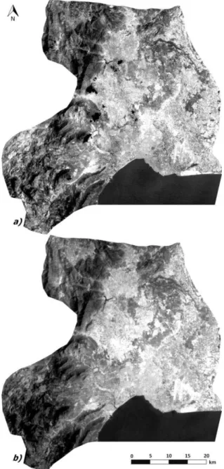
In this study, central districts of Antalya, which are Aksu, Dosemealti, Kepez, Konyaalti, and Muratpasa, are selected as study area (Figure 1). Antalya is the fifth biggest city of Turkey and its urbanization and population growth rates are quite high. Its population is about 205,000 in 2000 and 1,200,000 in 2014, for these five districts (TODAIE, 2016). Antalya is located in the southern part of Turkey and it is one of the most important tourism centers of the country. The city has Mediterranean climate with hot, dry summers and mild, wet winters. The summer population of Antalya increases almost double.
For this study, Landsat 7 ETM+ dated on June 5, 2001 and Landsat 8 OLI/TIRS dated on June 17, 2014 images were used as basic data for calculating the LST and determining the UHI effect. The Landsat images were provided from the USGS Earth Resource Observation and Science Centre (Global Visualization Viewer) and they have a Universal Transverse Mercator (UTM) coordinate system. Landsat 7 ETM+ satellite has 6 multispectral bands, 1 panchromatic band and 1 thermal band. On the other hand, Landsat 8 OLI/TIRS satellite has two new multispectral bands (Band1-deep blue coastal aerosol band and Band9-shortwave infrared cirrus band) in addition to Landsat 7 ETM+ spectral bands. Landsat 8 OLI/TIRS satellite has 2 thermal bands (Band10 and Band11). However, the wavelength ranges of Landsat 8 OLI/TIRS and Landsat 7 ETM+ are almost the same for thermal region. The Band 11 of Landsat 8 is not recommended for using in quantitative analysis (USGS, 2013). Therefore, Band 10 of Landsat 8 was used in this study as thermal band. Besides, radiometric resolution of Landsat 7 ETM+ images are 8 bit, while Landsat 8 OLI/TIRS images are 12 bit (USGS, 2015). Surface UHI is more apparent during the day of summer (EPA, 2014). UHI magnitude was observed that has to be higher in the summer in review of different studies (Hung et al., 2006; Imhoff et al., 2010). For this reason, the summer images were used in our study.
In addition to Landsat imagery, the topographic maps, ASTER GDEM, DMSP_OLS nighttime light data and MODIS/Terra LST and Emissivity data were used in this study. 1:100,000 scaled topographic maps were used for the geometric correction of the Landsat images. ASTER GDEM had been produced using stereo pair images collected by the ASTER satellite and it is a joint product made by publicly available by the Ministry of Economy, Trade and Industry (METI) of Japan and United States National Aeronautics and Space Administration (NASA). The DMSP_OLS nighttime lights data supplies lights containing city, town or residential lights and ephemeral event lights like fires and lightning. The DMSP_OLS image includes valuable information for mapping urban areas and it is useful for separating urban and non-urban areas (Elvidge et al., 2001; Gallo et al., 1995; NOAA_OLS, 2012; Sutton et al., 2010). The DMSP_OLS nighttime lights data was acquired from National Oceanic and Atmospheric Administration/National Geophysical Data Center (NOAA/NGDC) for the years 2001 and 2013. The NDVI image, ASTER GDEM and DMSP_OLS nighttime light data in addition to Landsat 8 OLI images were used for the classification procedure, the thermal bands were used for determining the LST values. On the other hand, the MODIS/Terra LST and Emissivity data was used for validation.
Figure 1. The false color Landsat 8 OLI/TIRS image of the study area and its location in Turkey.
3. METODHOLOGY
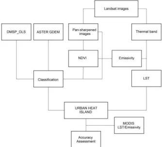
There are basically three main steps in this study, which are (1) pre-processing and preparation of additional bands for image classification, (2) LU/LC classification using RF Classifier and (3) calculation of the LST values and UHI effect using thermal images.
In the pre-processing stage the Landsat images were pan-sharpened and corrected geometrically. Later, auxiliary data, which are NDVI image, emissivity and enhanced DMSP_OLS nighttime lights data were generated. The generated NDVI image, enhanced DMSP_OLS nighttime lights data, and ASTER GDEM were used as additional bands during the RF classification procedure.
In the RF classification procedure, firstly, data sets were created using the original and additional bands (Table 1 and Table 2). According to classification results, the data sets that provides the highest overall accuracies for the years 2001 and 2014 were used for examining the relationship between the LU/LC classes The International Archives of the Photogrammetry, Remote Sensing and Spatial Information Sciences, Volume XLI-B8, 2016
and UHI values. The flowchart of the proposed UHI effect determination procedure is shown in Figure 2.
Figure 2. Flowchart of the UHI effect determination procedure
3.1 Pre-processing and preparation of additional bands for RF classification
In this study, firstly, Landsat multispectral imageries were pan-sharpened using the PANSHARP algorithm of PCI Geomatica image processing software. Then, the pan-sharpened Landsat imageries were geometrically corrected using Ortho Engine module of PCI Geomatica image processing software. In the geometric correction stage, the Landsat 8 OLI/TIRS images were corrected using topographic maps and its root mean square error was calculated less than 0.5 pixel. Afterward, image to image registration was performed to correct Landsat 7 ETM+ image geometrically using the Landsat 8 OLI/TIRS image and its root mean square error was calculated less than 0.5 pixel.
The NDVI image shows the density of vegetation in the study area. This image is useful for separating vegetation from other LU/LC classes. NDVI image was created using Near Infrared (NIR) and Red (R) bands in Landsat imagery using the following NDVI equation (Eq.1):
NDVI = (NIR - R) / (NIR + R) (1)
Emissivity is the radiation capability of objects and this value is between 0 and 1. In this study, typical emissivity value is 0.99 for full vegetative pixels. Emissivity values were calculated using the below given equations (Eq. 2) (Sobrino et al., 2008);
εsʎ εʎ = εsʎ+(εvʎ-εsʎ)*Pv εvʎ
NDVI < NDVIs NDVIs ≤ NDVI ≤ NDVIv NDVI > NDVIv
(2)
where; εʎ : emissivity, εsʎ: bare soil emissivity εvʎ: vegetation emissivity
The NDVIs and NDVIv values were approved as 0.2 and 0.5, respectively (Sobrino et al., 2008; Sobrino and Raissouni, 2000).
Pv values are calculated according to Eq. 3 (Carlson and Ripley, 1997);
Pv = (NDVI - NDVIs /NDVIv - NDVIs) ^2 (3) εsʎ = 0.980 - 0.042 * K (4)
K: DN values of red band,
εvʎ has been approved 0.99 and εsʎand εʎ has been calculated using the formulas given in (Sobrino et al., 2008; Sobrino and Raissouni, 2000).
Additionally, the DMSP_OLS nighttime lights image was enhanced using emissivity image, because of its spatial resolution is too low when compared with Landsat imagery. For this process, Landsat satellite image was analysed with emissivity and NDVI images. The non-urban areas were determined using the pixel values higher than 0.98 in emissivity image and pixel values lower than 0 in NDVI image. Therefore, these values were masked out by giving zero values to these pixels on DMSP_OLS image. The original and enhanced DMSP_OLS nighttime lights data were given in Figure 3.
Figure 3. DMSP_OLS nighttime lights data, original (a) and enhanced (b)
3.2 RF classification
The RF classification algorithm is suggested by Breiman (2001) and it is a supervised classification technique. RF classifier, which uses improved bagging and bootstrapping techniques, is based on decision tree. It includes huge amount of trees and each tree is grown from randomly chosen training pixels. In RF classification algorithm, there are two parameters that should be defined; k (number of trees to grow), and m (number of variables to split each node). RF and SVM (Support Vector Machine) classifiers are the most preferred machine-learning algorithms and their usage in remote sensing image classification is relatively new. RF and SVM classifiers are provides almost the same overall accuracies (Pal, 2005). On the other hand, RF classifier is not sensitive to noise or overtraining (Gislason et al., 2006). In addition, RF classifier is faster when compared with SVM classifier. Therefore, the RF classifier was preferred in this study.
The detailed RF classification procedure that we used was explained in the previous study performed by the authors (Aslan and Koc-San, 2015). In RF classification, NDVI, ASTER GDEM and DMSP_OLS nighttime lights data were used as additional bands and five and six data sets were formed for Landsat 7 and Landsat 8 (Table 1 and Table 2) classification procedures, respectively.
Landsat 7 ETM+ data sets Date set1 Pan-sharpened bands (Bands: 1-5, 7) Date set2 Pan-sharpened bands and NDVI image Date set3 Pan-sharpened bands and DMSP_OLS Date set4 Pan-sharpened bands and Aster GDEM Date set5 All bands
Table 1.The data sets showing band combination that used to RF classification of LANDSAT 7 ETM+ image
Landsat 8 OLI/TIRS data sets Date set1 Pan-sharpened bands (Bands: 2-7) Date set2 Pan-sharpened bands (Bands: 1-7, 9) Date set3 Pan-sharpened bands and NDVI image Date set4 Pan-sharpened bands and DMSP_OLS Date set5 Pan-sharpened bands and Aster GDEM Date set6 All bands
Table 2. The data sets showing band combination that used to RF classification of LANDSAT 8 OLI/TIRS image
After creating the data sets, thirteen classes, which are urban, industry, greenhouse, vegetation, irrigated agriculture, dry agriculture, rock, bare land, water, snow, cloud and shadow, were determined by analysing the imagery visually. Then, 300 and 600 pixels per class were collected as training and testing, respectively from different areas. The RF classification was applied using Image RF IDL based tool that is used for remote sensing image classification (Koc-San, 2013a, 2013b; Waske et al., 2012). This tool is freely available and license and platform independent (Waske et al., 2012). The k and m values were selected as 100 and square root of the number of all input properties, respectively.
3.3 Estimation of LST from Landsat 7 ETM+ and Landsat 8 OLI/TIRS images
To investigate the UHI effect on the central districts of Antalya city, the LST values were calculated using the Landsat thermal
images (Band 6 for Landsat 7 ETM+ and Band 10 for Landsat 8 OLI/TIRS Satellites)(Chen et al., 2006; Feng et al., 2014).
For this purpose firstly, the DN values were converted to spectral radiance (Lb) using Eq.5:
Lb = Lmin + (Lmax - Lmin) * DN/ (Qcalmax - Qcalmin) (5)
where:
Lb: Spectral radiance (W/(m
2*sr*µm))
Lmin and Lmax: minimum and maximum thermal radiation energy that was obtained from image Metadata file.
Qcalmin and Qcalmax: minimum and maximum quantized calibrated pixel values that were obtained from image Metadata file.
Then, the brightness temperatures were calculated using the below given formula (Eq. 6):
Tb = K2 / (ln(K1/Lb + 1)) (6)
Tb: brightness temperature
K1: thermal conversion constant for the thermal band K2: thermal conversion constant for the thermal band K and K constant are findable image Metadata file.
After that, the LST values were obtained from brightness temperatures (Artis and Carnahan, 1982; Weng et al., 2004);
Ts = Tb/ (1 + (ʎ * Tb/α) * lnε) (7)
Ts: land surface temperature (Kelvin) ʎ = 10.895 µm
α = 14388.15 µmK
ε: land surface emissivity (Sobrino et al., 2008)
Lastly, the LST values were converted from Kelvin to Celsius degrees unit using the following equation (Eq. 8).
T (°C) = Ts - 273.15 (8)
4. RESULTS
4.1 RF classification assessment
The obtained LU/LC thematic maps of Landsat 7 ETM+ and Landsat 8 OLI/TIRS imageries are illustrated in Figure 4. The overall accuracy values for Landsat 7 ETM+ and Landsat 8 OLI/TIRS imageries are given in Table 3 and 4, respectively. When the obtained results are analysed, it can be stated that the RF classifier provides quite accurate LU/LC results with computed overall accuracies over than 80% for almost all the data sets.
According to the obtained classification results, the two new bands of Landsat 8 OLI/TIRS satellite raised the classification accuracy about 1.6%. Using ASTER GDEM as additional band increases the classification accuracy mostly and this increase is about 4.5% and 7.4% for the years 2001 and 2014, respectively. Besides, DMSP_OLS nighttime lights data were increased the overall accuracy about 3.7% and 3.2% for the years 2001 and 2014, respectively. On the other hand, using the NDVI image as additional band effects the accuracies slightly.
Figure 4. Thematic LU/LC maps of 2001 Landsat 7 ETM+ (a) and 2014 Landsat 8 OLI/TIRS (b) imageries
When accuracy assessment results were analysed, it can be stated that using all additional bands in addition to original pan-sharpened bands provided highest accuracy results and overall accuracy values were computed as 88.66% for Landsat 7 ETM+ and 91.31% for Landsat 8 OLI/TIRS imageries. The usage of additional bands increased the classification accuracies over than 8% when compared to using only pan-sharpened bands.
Data sets
1 2 3 4 5
Overall acc.
80.16 79.93 83.93 84.68 88.66
Kappa coef.
0.78 0.78 0.82 0.83 0.87
Table 3. RF classification results for Landsat 7 ETM+ and additional bands
Data sets
1 2 3 4 5 6
Overall acc.
80.98 82.61 82.93 85.80 90.01 91.3 1 Kappa
coef.
0.78 0.80 0.81 0.84 0.88 0.90
Table 4. RF classification results for Landsat 8 OLI/TIRS and additional bands
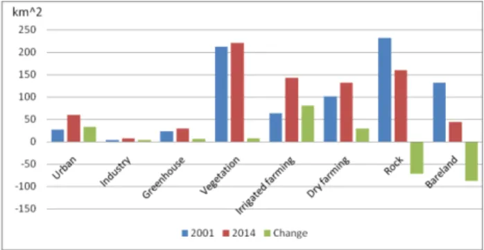
Additionally, LU/LC change was investigated between the 2001 and 2014 years. The LU/LC change detection results demonstrate that urban, industry, greenhouse, agriculture and vegetation areas were increased, while the rock and bareland areas were decreased (Figure 5).
Figure 5. The amount of LU/LC changes between the years 2001-2014 (x and y axis shows LU/LC types and areas,
respectively)
Furthermore, there are positive change rate about 120% for urban, industry and irrigated agriculture areas, whereas there is negative change rate approximately -66% for bareland areas and -31% for rock areas.
4.2 Relationship between LST and land use/cover type
The relation between the previously determined LST values and LU/LC classes is analysed in this section. For this purpose, the cloud, shadow, water and snow areas were masked out from the study area for Landsat 7 ETM+ and Landsat 8 OLI imageries. The higher LST values were observed in urban, industry, greenhouse, dry agriculture and bareland areas. On the other hand, the lowest LST values were observed in vegetation areas (Table 5 and Figure 6). The LST values were increased for almost all areas from 2001 to 2014. This increase is more than 4 °C for industrial and bareland areas and that is 3.6 °C, 3.4 °C, and 1.6 °C for urban, greenhouse, and vegetation areas, respectively. In contrast, the LST change is negative with -1.5 °C in rock areas.
Class LST value (°C)
(2001)
LST value (°C) (2014)
Urban 35.52 39.14
Industry 33.55 38.00
Greenhouse 34.01 37.50
Vegetation 29.45 31.07
Irrigated agriculture 30.44 33.89
Dry agriculture 36.35 39.20
Rock 31.89 30.33
Bareland 34.90 39.86
Table 5. LU/LC types and their LST values
Figure 6. Graph of the LU/LC types and their LST values The International Archives of the Photogrammetry, Remote Sensing and Spatial Information Sciences, Volume XLI-B8, 2016
4.3 Assessment of the UHI effect magnitude and validity of the study result
In this study, the UHI effect was determined by differencing the average LST values for built-up and green areas and this value was found about 5.6 °C and 6.8 °C for the years 2001 and 2014, respectively (Figure 7).
Figure 7. Land Surface Temperatures maps of 2001 Landsat 7 ETM+ (a) 2014 Landsat 8 OLI/TIRS (b) imageries.
The validity of the study was tested using MODIS LST/Emissivity data. MODIS LST values were rescaled by Eq. 9 (Odindi et al., 2015).
LST = (LSTI * 0.02) - 273.15 (9)
where:
LSTM: rescaled LST digital values
LSTI: original MODIS LST/Emissivity digital values
The correlation between the MODIS LST/ Emissivity data and the Landsat LST images were computed and it was observed
that the correlation values are quite high. The correlation values were computed as 0.7 for 2001 image (Landsat 7), while 0.9 for 2014 image (Landsat 8).
5. CONCLUSIONS
In the present study, the LST value and UHI effect changes were evaluated between the years 2001 and 2014 using Landsat imageries. The LST values were computed using thermal imageries of Landsat 7ETM+ (June 5, 2001) and Landsat 8 OLI/TIRS (June 17, 2014) imageries. In addition, the LU/LC thematic maps were created using RF classifier. The relation between the LST values and LU/LC classes were analysed. The study is implemented in the central districts of Antalya.
The LU/LC thematic maps’ overall accuracies were computed above 80%. It was observed that, the classification accuracies were increased when all auxiliary data were used in addition to the original Landsat bands and in this case the classification overall accuracies were computed as 88.66% and 91.31% for Landsat 7 ETM+ and Landsat 8 OLI/TIRS, respectively. Urban, industry, greenhouse, vegetation, irrigated agriculture and dry agriculture areas increased, while bareland and rock areas reduced significantly within 13-year time interval.
The world temperature is continuously increasing due to the global warming. In Antalya case, the LST values are also increased about 2.5 °C from 2001 to 2014, but this increase is not the same amount for each class. This increase is highest for bareland areas with 4.96 °C and it follows for industrial areas with 4.45 °C, for urban areas with 3.62 °C, for greenhouse areas with 3.49 °C, for irrigated agriculture with 3.45 °C. On the other hand, the LST value increases are relatively lower for dry agriculture, and vegetation classes, with the values of 2.85 °C, and 1.62, respectively. According to the obtained results, it can be said that the LST values vary depending on the surface property. Urban area is hotter than industrial area or vegetation area is colder than irrigated agriculture area. In addition to these cases, dry agriculture area is hotter than the irrigated agriculture area. Subsequently, the obtained results indicate that the LST value depends on the surface spatial property. The UHI effect was found as 5.6 °C and 6.8 °C for 2001 and 2014, respectively. Therefore, it can be stated that the UHI effect increased from 2001 to 2014 about 1.2 °C.
REFERENCES
Artis, D.A., & Carnahan, W.H., 1982. Survey of emissivity variability in thermography of urban areas. Remote Sensing of
Environment, 12, pp. 313-329.
Aslan, N., & Koc-San, D., 2015. The usage of combined Landsat 8 imagery and additional bands for random forest classification improvement. ASIAN CONFERENCE ON
REMOTE SENSİNG, pp. 1-9.
Breiman, L., 2001. Random forests. Machine Learning, 45, pp. 5-32.
Carlson, T.N., & Ripley, D.A., 1997. On the relation between NDVI, fractional vegetation cover, and leaf area index. Remote
Sensing of Environment, 62, pp. 241-252.
Chen, X.L., Zhao, H.M., Li, P.X., & Yin, Z.Y., 2006. Remote sensing image-based analysis of the relationship between urban The International Archives of the Photogrammetry, Remote Sensing and Spatial Information Sciences, Volume XLI-B8, 2016
heat island and land use/cover changes. Remote Sensing of
Environment, 104, pp. 133-146.
Effat, H.A., & Hassan, O.A.K., 2014. Change detection of urban heat islands and some related parameters using multi-temporal Landsat images; a case study for Cairo city, Egypt.
Urban Climate, 10, pp. 171-188.
Elvidge, C.D., Imhoff, M.L., Baugh, K.E., Hobson, V.R., Nelson, I., Safran, J., Dietz, J.B., & Tuttle, B.T., 2001. Night-time lights of the world: 1994-1995. Isprs Journal of
Photogrammetry and Remote Sensing, 56, pp. 81-99.
EPA (2014). Reducing Urban Heat Islands: Compendium of Strategies. In,
https://www.epa.gov/sites/production/files/2014-06/documents/basicscompendium.pdf (14 April 2016).
Feizizadeh, B., & Blaschke, T., 2013. Examining Urban Heat Island Relations to Land Use and Air Pollution: Multiple Endmember Spectral Mixture Analysis for Thermal Remote Sensing. Ieee Journal of Selected Topics in Applied Earth
Observations and Remote Sensing, 6, pp. 1749-1756.
Feng, H.H., Zhao, X.F., Chen, F., & Wu, L.C., 2014. Using land use change trajectories to quantify the effects of urbanization on urban heat island. Advances in Space Research, 53, pp. 463-473.
Gallo, K.P., Tarpley, J.D., Mcnab, A.L., & Karl, T.R., 1995. Assessment of Urban Heat Islands - a Satellite Perspective.
Atmospheric Research, 37, pp. 37-43.
Gislason, P.O., Benediktsson, J.A., & Sveinsson, J.R., 2006. Random Forests for land cover classification. Pattern
Recognition Letters, 27, pp. 294-300.
Hu, Y.S., & Jia, G.S., 2010. Influence of land use change on urban heat island derived from multi-sensor data. International
Journal of Climatology, 30, pp. 1382-1395.
Hung, T., Uchihama, D., Ochi, S., & Yasuoka, Y., 2006. Assessment with satellite data of the urban heat island effects in Asian mega cities. International Journal of Applied Earth
Observation and Geoinformation, 8, pp. 34-48.
Imhoff, M.L., Zhang, P., Wolfe, R.E., & Bounoua, L., 2010. Remote sensing of the urban heat island effect across biomes in the continental USA. Remote Sensing of Environment, 114, pp. 504-513.
Jimenez-Munoz, J.C., Sobrino, J.A., Skokovic, D., Mattar, C., & Cristobal, J., 2014. Land Surface Temperature Retrieval Methods From Landsat-8 Thermal Infrared Sensor Data. Ieee
Geoscience and Remote Sensing Letters, 11, pp. 1840-1843.
Jin, M.J., Li, J.M., Wang, C.L., & Shang, R.L., 2015. A Practical Split-Window Algorithm for Retrieving Land Surface Temperature from Landsat-8 Data and a Case Study of an Urban Area in China. Remote Sensing, 7, pp. 4371-4390.
Jin, M.L., Dickinson, R.E., & Zhang, D.L., 2005. The footprint of urban areas on global climate as characterized by MODIS.
Journal of Climate, 18, pp. 1551-1565.
Koc-San, D., 2013a. Evaluation of different classification techniques for the detection of glass and plastic greenhouses
from WorldView-2 satellite imagery. Journal of Applied
Remote Sensing, 7, pp. 073553-1-20.
Koc-San, D., 2013b. Thematic mapping of urban areas from WorldView-2 satellite imagery using machine learning algorithms. Journal of Geodesy and Geoinformation, 2, pp. 29-38.
Lo, C.P., & Quattrochi, D.A., 2003. Land-use and land-cover change, urban heat island phenomenon, and health implications: A remote sensing approach. Photogrammetric Engineering and
Remote Sensing, 69, pp. 1053-1063.
Mallick, J., Rahman, A., & Singh, C.K., 2013. Modeling urban heat islands in heterogeneous land surface and its correlation with impervious surface area by using night-time ASTER satellite data in highly urbanizing city, Delhi-India. Advances in
Space Research, 52, pp. 639-655.
NOAA_OLS (2012). Operational Linescan System. In: http://www.ngdc.noaa.gov/dmsp/sensors/ols.html, (14 April 2016).
Odindi, J.O., Bangamwabo, V., & Mutanga, O., 2015. Assessing the Value of Urban Green Spaces in Mitigating Multi-Seasonal Urban Heat using MODIS Land Surface Temperature (LST) and Landsat 8 data. International Journal of
Environmental Research, 9, pp. 9-18.
Oke, T.R., 1973. City size and the urban heat island.
Atmospheric Environment (1967), 7, pp. 769-779.
Oke, T.R., 1982. The Energetic Basis of the Urban Heat-Island.
Quarterly Journal of the Royal Meteorological Society, 108,
pp. 1-24.
Pal, M., 2005. Random forest classifier for remote sensing classification. International Journal of Remote Sensing, 26, pp. 217-222.
Rozenstein, O., Qin, Z.H., Derimian, Y., & Karnieli, A., 2014. Derivation of Land Surface Temperature for Landsat-8 TIRS Using a Split Window Algorithm. Sensors, 14, pp. 5768-5780.
Sekertekin, A., Kutoglu, S.H., & Kaya, S., 2016. Evaluation of spatio-temporal variability in Land Surface Temperature: A case study of Zonguldak, Turkey. Environmental monitoring and
assessment, 188, pp. 1-15.
Singh, R.B., Grover, A., & Zhan, J.Y., 2014. Inter-Seasonal Variations of Surface Temperature in the Urbanized Environment of Delhi Using Landsat Thermal Data. Energies, 7, pp. 1811-1828.
Sobrino, J.A., Jimenez-Munoz, J.C., & Paolini, L., 2004. Land surface temperature retrieval from LANDSAT TM 5. Remote
Sensing of Environment, 90, pp. 434-440.
Sobrino, J.A., Jimenez-Munoz, J.C., Soria, G., Romaguera, M., Guanter, L., Moreno, J., Plaza, A., & Martincz, P., 2008. Land surface emissivity retrieval from different VNIR and TIR sensors. Ieee Transactions on Geoscience and Remote Sensing, 46, pp. 316-327.
Sobrino, J.A., & Raissouni, N., 2000. Toward remote sensing methods for land cover dynamic monitoring: application to The International Archives of the Photogrammetry, Remote Sensing and Spatial Information Sciences, Volume XLI-B8, 2016
Morocco. International Journal of Remote Sensing, 21, pp. 353-366.
Sutton, P.C., Taylor, M.J., & Elvidge, C.D. (2010). Using DMSP OLS Imagery to Characterize Urban Populations in Developed and Developing Countries. In T. Rashed, & C. Jürgens (Eds.), Remote Sensing of Urban and Suburban Areas
pp. 329-348. Dordrecht: Springer Netherlands
Tayanc, M., & Toros, H., 1997. Urbanization effects on regional climate change in the case of four large cities of Turkey. Climatic Change, 35, pp. 501-524.
TODAIE, 2016. Antalya Ilçeleri Nufus Listesi.
http://antalya.yerelnet.org.tr/il_ilce_nufus.php?iladi=antalya,
(14 April 2016).
USGS, 2013. Upcoming change in Landsat 8 Radiometric Calibration (Revision). http://landsat.usgs.gov/calibration_
notices.php, (14 April 2016).
USGS, 2015. LANDSAT 8 (L8) DATA USERS HANDBOOK.
http://landsat.usgs.gov/documents/Landsat8DataUsersHandbo
ok.pdf, (14 April 2016).
Wang, F., Qin, Z.H., Song, C.Y., Tu, L.L., Karnieli, A., & Zhao, S.H., 2015. An Improved Mono-Window Algorithm for Land Surface Temperature Retrieval from Landsat 8 Thermal Infrared Sensor Data. Remote Sensing, 7, pp. 4268-4289.
Waske, B., van der Linden, S., Oldenburg, C., Jakimow, B., Rabe, A., & Hostert, P., 2012. imageRF - A user-oriented implementation for remote sensing image analysis with Random Forests. Environmental Modelling & Software, 35, pp. 192-193.
Weng, Q.H., Lu, D.S., & Schubring, J., 2004. Estimation of land surface temperature-vegetation abundance relationship for urban heat island studies. Remote Sensing of Environment, 89, pp. 467-483.
Yu, X.L., Guo, X.L., & Wu, Z.C., 2014. Land Surface Temperature Retrieval from Landsat 8 TIRS-Comparison between Radiative Transfer Equation-Based Method, Split Window Algorithm and Single Channel Method. Remote
Sensing, 6, pp. 9829-9852.