DETECTING AND EVALUATING LAND COVER CHANGE IN THE EASTERN HALF OF EAST TIMOR (1972 – 2011)

(1)

Guia para a formatação de teses Versão 4.0 Janeiro 2006

DETECTING AND EVALUATING LAND COVER CHANGE

IN THE EASTERN HALF OF EAST TIMOR (1972

–

2011)

(2)

Detecting and Evaluating Land Cover Change in the

eastern half of East Timor (1972

–

2011)

Dissertation supervised by

Prof. Dr. Mário Caetano (New University of Lisbon, Portugal)

Dissertation co-supervised by

Prof. Dr. Filiberto Pla (University Jaume I Castellon, Spain)

Prof. Dr. Edzer Pebesma (University of Münster, Germany)

(3)

ACKNOWLEDGEMENT

I am grateful to the European Union and Erasmus Mundus Consortium (Universidade Nova de Lisboa, Portugal , University of Münster, Germany and Universitat Jaume I, Spain) for awarding me the scholarship to undertake this course. It is a great opportunity for my lifetime experiences. I would like to sincerely thank my supervisor Prof. Mário Caetano whose hard work, guidance, advice and motivation helped realized my goal in this study. I would also like to thank my co-supervisors Prof. Dr. Edzer Pebesma and Prof. Dr. Filiberto Pla for finding time between their schedule to serve on my committee and for their support. This work is not possible without the help from Prof. Dr. Marco Painho who continued to be a constant guidance during the last few months.

(4)

DETECTING AND EVALUATING LAND COVER CHANGE IN THE EASTERN HALF OF EAST TIMOR (1972 – 2011)

ABSTRACT

Land use / land cover (LULC) change detection based on remote sensing (RS) data is an important source of information for various decision support systems. In East

Timor where forest plays a key role in sustaining communities’ livelihoods the

information derived from LULC change detection is invaluable to the conservation, sustainable development and management of forest resources.

To assess the patterns of land cover change, as a result of complex socio-economic factors, satellite imagery and image processing techniques can be useful. This study is concerned with identifying change in land use and land cover types in East Timor between 1972 and 2011, using satellite images from Landsat MSS, TM and ETM+ sensors. Seven major cover types were identified in this study including forest, mixed rangeland, grassland, farmland, built-up areas, bare soil and water. A combination of NDVI differencing, supervised and unsupervised classification was used to derive final classification maps. Due to the lack of ground truth data, further processing were performed to improve the final classification maps by applying rationality change test.

(5)

KEY WORDS

Change Detection

Change Rationality Test

Landsat

Land Use/Land Cover

(6)

ACRONYMS

DN Digital Number

DOS Dark Object Subtraction

ETM+ Enhanced Thematic Mapper Plus

FAO Food and Agricultural Organization

FCC False Color Composite

GLOVIS Global Visualization Viewer

LULCL Land Use/Land Cover

MAF Ministry of Agriculture and Fisheries

MLC Maximum Likelihood Classification

MSS Multispectral Scanner

NDVI Normalized Difference Vegetation Index

NIR Near Infrared

TCC True Color Composite

TM Thematic Mapper

TOA Top-of-Atmosphere

UTM Universal Transverse Mercator

(7)

LIST OF TABLES

Table 2.2.1. Raw Landsat data used in this study……….... 9

Table 2.2.2. Reference data ………. ………. 10

Table 5.2.1. Thresholds of index decrease and increase for all NDVI differencing images………... 37

Table 5.3.1. One time accuracy assessment for 2000 image……….…….… 41

Table 5.4.1.1. Total number of unchanged pixels for each category as defined by Rule I …………...……….…. 42

Table 5.4.3. Summary of change rationality test……….. 43

Table 5.5.1. Summary of final classification map area statistics for six observation dates………..………...…... 44

Table 5.5.2. The percentage of land use categories for each observation date... 45

Table 5.6.1. Matrix of land cover change from 1972 to 1987………..….. 46

Table 5.6.2. Matrix of land cover change from 1987 to 1996……… 47

Table 5.6.3. Matrix of land cover change from 1996 to 2000……….…... 48

Table 5.6.4. Matrix of land cover change from 2000 to 2005………...…. 48

(10)

LIST OF FIGURES

Figure 1.2. Vegetation distribution in western part of East Timor in 1989………. 4

Figure 1.2. Vegetation distribution in western part of East Timor in 1999…………... 4

Figure 2.1. Map of the study area………...……….. 8

Figure 4. The main workflow of the methodology………... 17

Figure 4.1.1. Landsat ETM+ 2011 band 5 with before gap filling……….. 19

Figure 4.1.2. Landsat ETM+ 2010 band 5 used for filling the gaps in 2011 image ...20

Figure 4.1.3. The result of gap-filling procedure for 2011 image band 5 ………..20

Figure 4.2. The rescaling factors contained in the product metadata of Landsat TM5

acquired on October 11, 2005. ………..……….. 23 Figure 4.2.1. Probability density function of NDVI differencing image……….……….. 30

Figure 4.2.1.1. Range of optimal c value.……….………... 31

Figure 4.2.2. Derivation of final classification maps for five acquisition dates (1972,

1987, 1996, 2005 and 2005) by combining change/no change maps and classified

maps from supervised and unsupervised methods………..………33

Figure 5.1.1. NDVI maps for all observation dates………..…. 38

Figure 5.3.1. NDVI index decrease part shows large amount of noises due the

selection of high c value (smaller negative). The blue circle shows and airport

run….………..….. 39

Figure 5.3.2. NDVI index decrease part shows minimum noise due to selection of

low c value (larger negative). ………..……….……….…. 40

Figure 5.3.3. NDVI index decrease part using medium c value. Notice the reduction

(11)

Figure 5.4.1.1. Unchanged LULC categories between 1972 and 2011 as identified by

change rationality test……….. 42

Figure 5.5.1. Distribution of land cover types in East Timor between 1972 and

2011………. 45

Figure 5.6.1. Gain and loss of LULC change classes between 1972 and 2011……….,50

Figure 5.6.2. “From-to” major categorical change map between 1972 and 2011…. 50

Figure 5.6.3. “From-to” change between 1972 and 2011 in Lautem district………... 51

Figure 5.6.4. “From-to” change between 1972 and 2011 in Baucau and Viqueque

(12)

CHAPTER 1 INTRODUCTION

1.1. Background

Research focus on land use and land cover (LULC) change gained prominence after

the realization that land cover change affects climate (Lambin et al., 2003). Since

then, many studies have been conducted around the world to understand the

causes, impacts and rates of land cover change. It is an important variable in

studying the dynamic changes that are continuously occurring on the earths’

surface. In addition, it has become a major issue in many of the current strategies

for managing natural resources and monitoring environmental damages. The

development of the concept of LULC has greatly increased research on land use and

land cover change, thus providing an accurate evaluation of the spread and health

of the world's forests, grasslands, and agricultural resources.

Worldwide deforestation is still alarmingly high (FAO, 2010). A recent study by

Goldewijk and Ramankutty (2004), where they assessed historical land cover data,

showed that forest has decreased from 50-62 million km2_{in 1700 to 43-53 million}

km2 _{in 1990. This reduction is due to the expansion in land used for crops and}

ranching (Goldewijk and Ramankutty, 2004). Many of these phenomena occur in

developing countries where agricultural expansion has caused reduction in forest

cover over long periods of time. In Brazil, for instance, the European exploitation of

forest for rubber plantation followed by sugar cane production caused the

reduction in Araucaria forest from 25 million ha to only 445000 ha. The

introduction of new cash crops to Brazil in 19th_{century contributed to the}

conversion of millions of hectares of forest into coffee plantation, adding more

(13)

included increased erosion problems on hill slope and disturbance to drainage

systems (Goldewijk and Ramankutty, 2004).

The examples above are just some of the many cases of causes and impacts of land

use/land cover changes. Obviously, deforestation in smaller countries may not be

heard of. However, the impacts are the same in the way that they affect

communities. Often times, the LULC change in an area is an outcome of complex

socio-economic condition in which human activities play a central role. Forest as a

resource is becoming scarce because of the immense agricultural expansion and

demographic pressure. Understanding this dynamic requires a tremendous amount

of resources in terms of time, finances, and the right technology, not only because

the problems are complex but also because it is geographically extensive in nature.

Thus, satellite images and aerial photography offer the most cost effective method

for land cover mapping and change detection throughout the world, both for

bi-temporal and multi-bi-temporal analysis (Ioannis and Meliadis., 2011). Over the years,

remote sensing in the form of aerial photography has been an important source of

LULC information. Ioannis and Meliadis (2011) state that this approach provides

several advantages: (1) the synoptic view of large geographic areas, (2) the digital

form of the data facilitating more efficient analysis and (3) land cover maps can be

generated at considerably less cost than by other methods. The cost of aerial

photography acquisition and the interpretation of cover types is prohibitively

expensive for extensive geographic areas, thus, a common alternative is to acquire

the needed information from freely available digital satellite imagery such as

Landsat TM and ETM+.

Hence, Remote Sensing (RS) and Geographic Information System (GIS) are now

providing new tools for better LULC studies. The collection of remotely sensed data

facilitates the synoptic analysis of Earth’s surface and its change at local, regional

(14)

1.2. Statement of the Problem and Justification

Like many other poor and developing countries around the world, forests play a

major role in sustaining agricultural-based communities’ livelihoods in East Timor.

The majority of people in East Timor practices shifting cultivation, by clearing and

burning of lands and cutting of forests and bushes. Coupled with wildfires and

excessive logging activity, this has caused a serious environmental problem

(Sandlund et al, 2001; Bouma and Kobryn, 2004). These traditional agricultural

practices have been around since at least 19th_{century and studies have indicated}

its intensification in recent years (Jeus et al., 2012). Yet, there has not been many

studies to understand the impact of such a practice on forest and so public

awareness of its impact is very low. This clearly poses serious challenges for the

task of efficient planning and management of the environment, which is often

constrained by insufficient information on the rates of land cover/use change.

As a relatively new nation, East Timor is facing great challenges and developmental

issues in many areas. One of the key areas concerns the dynamic of land use and

changing land cover situation which has not been given enough attention since the

country’s independence in 2002. Previous studies on land use/cover change in

East Timor have only looked at the phenomena between two different dates (i.e.

bi-temporal analysis). For instance, Bouma and Kobryn (2004) compared two

classified Landsat images (1989 and 1999) of the western part of East Timor and

found that the major vegetation cover types such as forest and woodland have

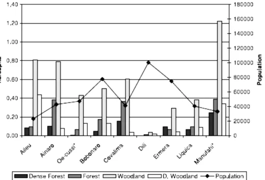
declined in nine districts (Figure 1 and 2). Mapping projects, conducted through

collaboration between public institutions and non-governmental agencies, have

also produced some spatial data, but only for recent years. Although, findings from

these studies have identified the common causes of environmental damages, and

have initiated the development of some key environmental policies, they are still

(15)

Figure 1.1. Vegetation distribution in western part of East Timor in 1989. Source: Bouma and Kobryn (2004).

(16)

The limited availability of historical data (e.g., land use maps, topographic maps,

aerial photos) in East Timor, the high cost of good quality data collection and

information dissemination, as well as the limited number of trained personnel in

remote sensing constrain East Timor’s ability to conduct LULC change detection

studies, or environmental studies in general. This challenge needs to be addressed

and overcome with viable solution.

A multi-temporal analysis of land cover change is deemed valuable in this regards.

By studying land use/cover change through multiple time stamps, a generalized

understanding of causes of land use/cover change over a longer trajectory can be

obtained. Freely available satellite data such as Landsat images can make it

possible to carry out this kind of study and the result from such a study can add to

the public’s knowledge the importance of spatial data and information for policy

making

1.3. Objective of the Study

The aim of this study is to analyze and detect land cover change using

multi-temporal Landsat images covering the eastern half of East Timor from 1972 to

2011. Specifically, the following questions will be used as guide in the study:

 What are the extent and nature of vegetation distribution in the eastern half

of East Timor?

 How is the vegetation trend changing during the study period in respect to

other cover types?

 Can land cover and land use change be mapped with limited reference data?  Is there an alternative to assess the accuracy of change detection derived

from limited reference data?

Furthermore, specific tasks will be performed to help answer the above questions.

 Calculate Normalized Difference Vegetation Index (NDVI) for all the

(17)

 Map land use and land cover types in the study region using commonly used algorithm such as supervised classification and/or unsupervised

classification techniques

 Perform and combine NDVI differencing techniques with LULC map to improve image classification result

(18)

CHAPTER 2

STUDY AREA AND DATASET

2.1. Study area

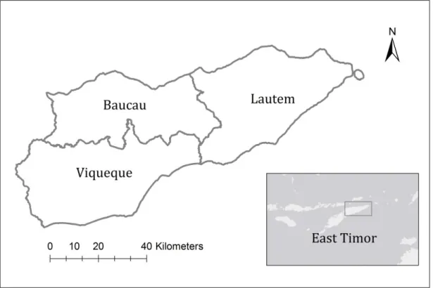
The study area is located in the eastern part of East Timor extending between

E126°, S8.3° and E127.5°, S9.1°. It covers three districts, Baucau, Viqueque and

Lautem (Figure 2.1). The topography of the region is highly varied characterized by

hilly terrain and coastal plains. The highest point in the region, which is also the

second highest point in East Timor, is mount Matebian (2335m). The rainfall

distribution in the study area also varies. In Baucau, precipitation is well

distributed in the hilly areas but less so near the coast. In Viqueque district rainfall

is well distributed throughout the area. Sometimes the rainy season (wet season) in

this area is longer than its dry period. According to the 1970 census by Portuguese

government the population in the study area was 177688, approximately 29.3% of

the total East Timor’s population (Costa Carvalho, 1970). The current population is

estimated at 241517 people of which 83% live in rural areas (NSD, 2011).

Agricultural land use in this region is predominant with Baucau and Viqueque

among the four districts in East Timor that produce 75% of the country’s rice

(Pederson and Arnerbeg, 1999). Another local product includes maize which is

grown in tilled fields or with little cultivation under traditional slash and burn

systems (Da Costa, 2003). Toward the eastern part of the study area is Lautem, the

district with much less agricultural intensification. In the past, however Lautem had

been an important livestock and fish producing area. A large portion of forested

land in the study area is located in Lautem where the first National Park was

established. This area is also home to 3 out of the 15 identified “important bird species” in East Timor (Mau, n.d.). Little is known about whether or not

(19)

Apart from the existence of deforestation in the area and the author’s familiarity of

the area, one of the reasons for selecting this study area is because a similar study

was already conducted on the western part of East Timor by Bouma and Kobryn

(2004) from which these three districts were excluded. Therefore, this study can be

used to enrich information regarding land use/cover change for the entire country

of East Timor.

Figure 2.1. Map of the study area

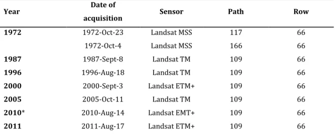
2.2. Dataset

This study spans a four decade time period—1970s, 1980s, 1990s, and 2000s. For

the 1970s two Landsat MSS images from October 4 and October 23, 1972 were

obtained to cover the entire study area. For the 1980s a Landsat TM image from

September 8, 1987 was obtained. For the 1990s, a Landsat TM image from August

15, 1996 was obtained. For the 2000s, the ETM+ image was obtained for the year

2000 and 2011, while for the year 2005, the Landsat TM image was used (Table

(20)

at the same time of day, being that all of the data is from Landsat that is not an

issue. Images with corresponding anniversary dates, which are dates over time

which correspond with season, month, and preferably weeks should be obtained

because it helps minimize discrepancies in reflectance caused by seasonal

vegetation fluxes and sun angle. However, often times anniversary dates are

impossible to obtain because of the times that the sensor system passes over a

particular area so the logical alternative is to find images of the area in the same or

near to the same month or season (Jensen 2007) In addition, atmospheric

conditions can also affect a sensor’s visibility as clouds tend to be persistent over a

tropical island such as East Timor. These issues were taken into consideration and

formed the basis for deciding the dataset for this study. All data was obtained from

the USGS Global Visualization Viewer (GLOVIS). Table 1 and 2 shows the

description of the data.

The reference data utilized in this study is a topographic map of East Timor with

the scale of 1:5000 and the 2000 land use map of East Timor. Both maps contain

information of land cover types for the year 2000. The land use map was produced

by the Ministry of Agriculture and Fisheries (MAF) using spot images with ground

truth data.

Year Date of

acquisition Sensor Path Row

1972 1972-Oct-23 1972-Oct-4 Landsat MSS Landsat MSS 117 166 66 66 1987 1987-Sept-8 Landsat TM 109 66 1996 1996-Aug-18 Landsat TM 109 66 2000 2000-Sept-3 Landsat ETM+ 109 66 2005 2005-Oct-11 Landsat TM 109 66

2010* 2010-Aug-14 Landsat EMT+ 109 66

2011 2011-Aug-17 Landsat ETM+ 109 66 Table 2.2.1. Raw Landsat data used in this study

(21)

Reference data Date of production Source Scale

Land use map of

East Timor 2000

ALGIS, Ministry of Agriculture and Fisheries

(MAF)

NA

Topographic map 2001 Ministry of Justice of East

Timor 1:50000

Table 2.2.2. Reference data

Tools

ArcGIS 10

(22)

CHAPTER 3

LITERATURE REVIEW

3.1. Remote sensing application

Since the advent of the remote sensing satellite (Landsat 1) in 1972, many land

cover and land use change studies started being conducted at varying levels. For

instance, at local level, studies were conducted in various domains including

landscape, agriculture, watershed management, forestry, and using data from

various sensors such as Landsat, MODIS and AVHRR. Masek et al (2000) used

Landsat images acquired between 1973 and 1996 to study land use efficiency in the

metropolitan area of Washington DC, USA. By applying NDVI differencing and

visual inspection of true urban growth, their study revealed that the Washington

metropolitan area has expanded at a rate of 8.5 square miles every year.

Doraiswamy et al, (2003) evaluated the integration of Landsat TM data into a crop

growth model to simulate wheat yields in the semi-arid region of North Dakota,

USA. Their study found similar result as the one reported by the county. Rahman et

al (2004) used Landsat (MSS, TM and ETM+) images to detect changes in winter

crops in Durgapur Upazilla, Bangladesh. Using the Maximum Likelihood Classifier

(MLC), they found an increasing trend in winter crops 1977 and 2000 which is

attributed to the increase in irrigation during winter season as well as population

pressure in the area. Petit et al (2001) also used MLC for a change detection study

in south-eastern Zambia, and reported an annual rate of 4.0% land cover change.

Another study was conducted by Anderson et al (2012) using moderate resolution

satellite imageries for the purpose of water resource management. Their study

concluded that Landsat thermal imagery can improve our ability to monitor

(23)

At regional level, application of remote sensing has also engaged in a wide range of

domains including deforestation, desertification and climate change among many

other things. For instance, Symeonakis and Drake (2004) developed a system for

monitoring desertification using four indicators (rainfall, vegetation cover, surface

run-off and soil erosion) that were derived from continental-scale remotely sensed

data. By combining theseindicators, they were able to identify areas under threat of

desertification. Another example of regional level application of remote sensing

study was the study on impacts of global warming in Arab region where MODIS

images were used (Ghoneim, 2009). CORINE Land Cover Mapping is also among the

many projects that entail regional collaboration to produce land cover maps based

on the interpretation of satellite images (EEA, 2013).

3.2. Change detection techniques

Over the years, a number of change detection techniques have been developed and

widely used for monitoring land use/land cover changes. Numerous researchers

have discussed the strength and weaknesses of each of this technique (Singh, 1989;

Nelson, 1983; Lu et al, 2004). These techniques can be broadly divided into two

main categories: pre-classification spectral change detection and post-classification

comparison techniques (Nelson, 1983; Singh, 1989, Coppin and Bauer, 1996).

Previous studies have successfully employed many of these techniques in analyzing

land cover change. Some of these studies have also focused on comparing the

ability of various techniques to accurately identify areas of change.

3.2.1. Pre-classification change detection technique

The pre-classification change detection technique is also referred to as

enhancement change detection. Generally, the pre-classification change detection

has the ability to accurately identify areas of spectral changes (Singh, 1989).

However, this technique requires additional analysis to determine the nature of the

(24)

co-registration. One of the most widely used change detection algorithm is image

differencing. It is a technique by which images captured at different times, which

are co-registered, are subtracted from one another to obtain unchanged areas.

Basically, it subtracts the Digital Number (DN) values of one band in the first image

from the corresponding DN value of the same band in the second image. The

subtraction results in positive and negative values for areas that change between

the two images and zero value for areas that do not change (Sohl, 1999). A critical

element of using this technique is how to decide where to place the threshold for

change in the differenced image (Singh, 1989). Additionally, it is also important to

apply radiometric normalization to the images before conducting image

differencing. Simplicity and straightforwardness are the strength of this technique

(Lu et al, 2004). However, it is quite sensitive to miregistration and mixed pixels

and it also lacks the information on the type of change that is occurring (Sohl, 1999;

Lu et al, 2004).

MacLeod and Congalton (1998) performed a quantitative comparison of change

detection algorithms and reported that image differencing performed better in

detecting changes in submerged aquatic vegetation, with an overall accuracy of

78%. However, Sohl (1999) and Veettil (2012) showed that the image differencing

technique was straightforward but on the expense of detailed information, and its

implementation can get more complicated when applied to multiple bands, due to

the difficulty of interpreting the colors of multi band false color composite. Hence,

Sohl (1999) states the simplicity of image differencing is also its main weaknesses

because it does not provide adequate explanation on the nature of the change.

Similar to image differencing is the vegetation index differencing. This technique

uses a data transformation shown to be related to green biomass where, for two

different dates, a Normalized Difference Vegetation Index (NDVI) image is

(25)

change and no-change (Mas, 1999). The NDVI is calculated by NDVI = (NIR –

RED)/(NIR + RED), where NIR represents near-infra red band response for a given

pixel of and RED represents red band (Mass, 1999). This method is also widely

used in land cover change studies (Pu et al, 2008; Masek et al, 2000).

3.2.2. Post-classification comparison

The post classification technique involves a comparative analysis of spectral

classification of two independently classified maps (Mas, 1999). This technique has

the advantage of providing direct information on the nature of land cover changes

and it can be used with both supervised and unsupervised classifications. The main

advantages of these techniques are that it minimizes atmospheric influences on the

images, and also the sensor and environmental differences between multi-temporal

images (Lu et al, 2004). This technique is capable of producing descriptive

information on the type of changes that are occurring, and it does not necessarily

require co-registration and radiometric normalization of input images. Lu et al

(2005) states that the disadvantages of this technique are that it requires great

amount of time and skills to produce classification, and that the accuracy of the

change detection depends on the accuracy of the classified maps because any

errors made in the classification are compounded into the change detection.

Numerous studies have produced good results with post-classification comparison

technique. Sohl (1999) reported accuracies of 96% for the identification of new

forest land and 62% for new agricultural land using a post classification technique

in a semi-arid environment. Guo et al (2010) also used post-classification

comparison by which they obtained an accuracy of 89% in their study of land cover

change to detect bushfire. Mersten and Lambin (2000) found a net reduction in

forest cover between 1973 and 1996 in Cameroon using post-classification

comparison technique. Furthermore, Sohl (1999) also noted the advantage of

(26)

between images. A comparative study of change detection techniques by Mas

(1999) also showed a high accuracy by post-classification comparison technique

which was attributed to the high accuracy of the classification of each individual

image.

While large number of studies has produced positive results with this technique,

MacLeod and Congalton (1998) reported that the post classification comparison

technique produced rather poor results compared to NDVI differencing, and they

stated that this poor accuracy could be attributed to the errors from both

classifications. In the review of change detection techniques Singh (1989) cited Toll

et al (1980) by stating that the poor performance of post-classification comparison

technique is partly due to the difficulty of producing image classifications that are

comparable to one another. With that said, there is no single image classifier or

change detection technique that fits every situation. Often times, researchers

perform comparison analysis of their performances and then decide to use the

classifier or technique that produces the best result.

3.3. Accuracy assessment

Accuracy assessment, then, is an important step in image classification and change

detection (Congalton and Green, 2008). A classified image or change detection map

needs to be compared against reference data, assumed to be true, in order to assess

its performance and quantify its accuracy. One of the common procedures in

describing the accuracy of a classified map is by using a confusion matrix where a

set of categories on a classified map and a reference map are plotted on a matrix

from which descriptive measures can be obtained (Congalton and Green, 2008,

Lillesand et al, 2004). Generally, a full accuracy assessment needs to include the

report on User Accuracy, Producer Accuracy and indices such as Kappa (Congalton

and Green, 2008). Pontius and Millones (2011), however, critically argued against

(27)

interpretation. Instead, they proposed the use of quantity disagreement and

allocation disagreement to obtain useful summary of the accuracy. Either way,

accuracy assessment for a successful remote sensing project relies heavily on the

reference data (Congalton and Green, 2008).

In multi-temporal studies where data spans over a long period of time, obtaining

reference data for multiple observation dates can be difficult. This certainly poses

challenges for change detection studies especially in areas where land use/land

cover information and reference data are of poor quality or even non-existent. This

problem has been discussed by numerous researchers (Liu and Zhou, 2004; Baraldi

et al, 2005; Foody, 2010) and while these authors recognize the utmost importance

of reference data, they have also shown that change detection can be performed

when the reference data are limited. Foody (2010) even concluded that it is

possible to estimate the accuracy of change detection without ground data. Liu and

Zhou (2004) on the other hand have proposed methodology for evaluating land

cover change trajectories where a set of rules can be defined to evaluate the

rationality of land cover change. This study will employ a slight modification of the

(28)

CHAPTER 4

METHODOLOGY

This section describes the methodology used in this study. First, various works in

the preprocessing stage (gap-filling, radiometric and atmospheric correction) are

described then followed by explanation of NDVI differencing technique and image

classification procedures. Finally, the explanation on change rationality test for

improving the final classification maps is presented. Figure 4.1 shows the main

workflow of the methodology.

(29)

4.1. Image Pre-processing

Prior to performing image classification it is important that the raw data are

preprocessed and prepared in a proper way so that error due to the geometry of

the earth, radiometric and atmospheric effects can be accounted for. The general

procedure in the preprocessing stage is to apply geometric, radiometric and

atmospheric correction. In this study the geometric correction was not applied to

the satellite images because they were already georeferenced to UTM Coordinate

System Zone 52S. Similarly, the land use shapefile from ALGIS was also

georeferenced. Thus, georeferencing was only performed for the scanned

topographic map of the study area, which resulted in a root mean square error

(RMSE) of 0.1123.

In addition, prior to radiometric and atmospheric corrections, which is described in

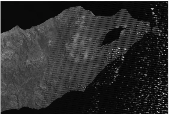
the following section, a Gap-filling was performed for Landsat image of 2011. This

image of 2011 was captured by Landsat ETM+. Due to its faulty Scan Line Corretor

(SLC) since 2003, the Landsat ETM+ sensor has been obtaining images of the

earth’s surface in the SLC-Off mode (Scan Line Corrector). As a result, the image only has about 87% of their pixels causing gap effects. These gaps created a

stripping effect along the edge of the image (Figure 4.1.1). Several procedures have

been developed to fill in these gaps including the work by Zhang et al., (2007) and

Scaramuzza et al., (2004). In this study the gap in the 2011 image was filled with

another Landsat ETM+ image which was acquired on August 14, 2010 (Figure

4.1.2). Each band in the 2011 image was filled with pixel information from its

corresponding band in the 2010 image. Although the 2010 image also has gaps, it

was possible to gap-fill the first image because the gaps in the images from two

different dates are not necessarily in the exact same spot. It is important to note

that the ideal procedure would be to use the image from the nearest month (e.g.,

September or October), however, due to the lack of cloud free image, the 2010

(30)

small enough to still make comparison with other decades using this data (Figure

4.1.3). This process of gap-filling was executed in the PANCROMA software using

the Hayes method. The Hayes method is a local optimization method where it uses

a sliding window technique, with a defined size, to estimate the value in the gaps

using values from other pixels that exist in the sliding windows (PANCROMA,

2012).

(31)

Figure 4.1.2. Landsat ETM+ 2010 band 5 used for filling the gaps in 2011 image

(32)

4.1.1. Cloud Masking

Clouds are a common feature found in all satellite images and they can affect image

classification because they may cover large extensive area under study. The easiest

way to deal with cloud cover is to include it in the classification as a separate class

or by masking the clouds outs. Most Landsat data used in this study have a very

minimum cloud cover. Yet, some clouds do exist and they were removed by using

techniques proposed by Martinuzzi et al. (2007).

The algorithm uses pixel information from band 1 (blue) and band 6 (thermal) to

create the mask. Clouds are very reflective in the blue band and very cold in the

thermal band. This method was chosen because it is an efficient and relatively

simple algorithm to create cloud mask for Landsat images. A prior visual analysis

was performed to identify the DN of clouds ranging from the minimum to 255. In

band 1 (blue) clouds are very reflective such that their DN are very high. Thus by

identifying pixel values where clouds appear thinner the mask was created where

DNmin<DN of pixel in band 1 < 255. In the thermal band (6), clouds are colder and

appear dark on the image. Hence, the mask was created for pixels where 1 >DN of

pixels in band 1 <DNmax.

By intersecting these two masks, and with an additional buffer of 3 pixels, final

cloud masks were obtained for images that have cloud contamination (1996, 2000,

2005). The masks were then used on the final classified maps to exclude pixels

from images which did not contain clouds so that they can be compared with

images that have clouds.

4.1.2. Conversion to at-sensor radiance (

When working with images data from multiple sensors and platforms it is

necessary to convert them into a physically meaningful common radiometric scale

(33)

calibration methods to scale, convert and store data. Radiometric calibration of

MSS, TM and ETM+ sensors involves rescaling raw digital numbers (Q) transmitted

from satellite to calibrated digital numbers (Qcal), which have the same

radiometric scaling for all scenes processed on the ground for a specific period.

Conversion from Qcal in Level 1 products back to at-sensor spectral radiance (Lλ)

requires knowledge of the lower and upper limit of the original rescaling factors.

The following equation is used to perform the Qcal-to-Lλ conversion for Level 1

products:

(1)

where

(2)

(3)

Therefore equation 1 can be rewritten as:

( (4)

where

= spectral radiance at the sensor’s aperture [W/m2_{sr µm)}_]

= quantized calibrated pixel value (DN)

= minimum quantized calibrated pixel value corresponding to [DN]

= Maximum quantized calibrated pixel value corresponding to [DN]

Spectral at-sensor radiance that is scaled to [W/(m2_{sr µm)}_]

= Spectral at-sensor radiance that is scaled to [W(/m2_{sr µm)}_]

(34)

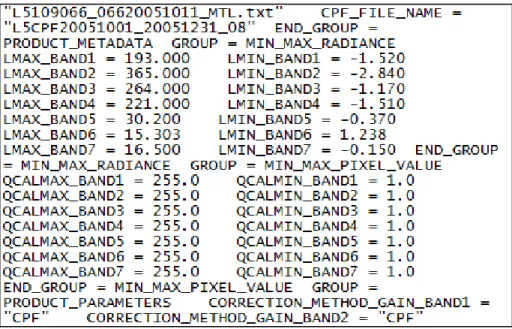
Information of this rescaling factor for Landsat data are contained in the header file

(.MTL). Figure 4.2. shows an example of rescaling factors for Landsat TM image

used in the study. Complete rescaling factors and radiometric calibration

coefficients for all the images can be seen in Appendix C.

Figure 4.2. The rescaling factors contained in the product metadata of Landsat TM5 acquired on October 11,

2005.

4.1.3. Conversion to at-sensor Radiance ( - )

Images acquired on different dates have different solar zenith angle, different

Earth-Sun distance, and different exoatmospheric solar irradiance that arise from

spectral band difference. Hence, they introduced scene-to-scene variability, which

can be improved by further processing. This can be done by converting at-sensor

radiance to exoatmospheric Top-of-Atmosphere (TOA) reflectance, also known as

in-band planetary albedo. Chander et al. (2009) mentioned that the TOA reflectance

helps remove the cosine effect of different solar zenith angle and compensates for

(35)

variation in the Earth-Sun distance between different data acquisition dates. The

TOA reflectance of the Earth is computed according to the equation:

(5)

where

= planetary TOA reflectance [unitless]

= Mathematical constant equal to ~3.14159 [unitless]

= Spectral radiance at the sensor’s aperture [W/m2_{sr µm)}_]

= Earth-Sun distance [astronomical units]

= Mean exoatmospheric solar irradiance [W/m2_{sr µm)}_] = Solar zenith angle [degrees]

4.1.4. Atmospheric correction by Dark-Object Subtraction (DOS)

The atmosphere affects images by scattering, absorbing, and refracting light and

these effects are wavelength dependent. Several methods are available to correct

for this effect including the Dark-Object Subtraction (DOS) technique. The DOS

atmospheric correction is an image-based technique, hence it does not require an

in-situ measurement during the acquisition of satellite images (Chavez, 1988;

Chavez, 1996). This technique assumes that there is high probability that there are

at least a few pixels within an image which should be black (0% reflectance), for

example, areas of shadow caused by topography or clouds in the image where the

pixels should be completely dark. Ideally, an imaging system should not detect

radiance at these shadow locations, and a DN value of zero should be assigned to

them. However, because of the atmospheric scattering effect, these shadowed areas

will not be completely dark and the sensor records a non-zero DN at these

locations. The value of DN at this location is assumed to be the haze value and needs to be subtracted from the particular band to account for atmospheric

(36)

on the Earth’s surface that are completely dark and so an assumption needs to be

made that these objects have at least one-percent of reflectance.

Therefore assuming that there are some dark objects whose reflectance are

supposed to be around zero, then the minimum DN value need to be subtracted

from all the pixels so that atmospheric effect can be removed from the entire image.

Sobrino et al. (2004) express the path radiance (atmospheric scattering) as:

(6) Where

is radiance that corresponds to a DN value for which the sum of all pixels with DN value lower or equal to this value is equal to the 0.01% of all the pixels from the

image considered (Sobrino et al., 2004, p.437). This radiance value can be obtained

using equation 4.

is the radiance of dark object assumed to have reflectance value of 0.01.

Therefore, and can be expressed like the following:

(7)

(8)

And the path radiance can be obtained by substituting equations 7 and 8 into

equation 6:

(9)

Chavez (1996) computed the variables , and to be the following:

= 1

(37)

This is assuming the no atmospheric transmittance loss, and corrects for the

spectral band solar irradiance and solar zenith angle, resulting in:

So, by substituting these values into equation 9, the path radiance (atmospheric

scattering) can be obtained by:

(10)

Finally, to obtain the surface reflectance of Landsat images equation 10 is

substituted into equation 5 as expressed below:

(11)

Where is defined by equation 4, is defined by equation 10, is the Earth-Sun

distance in astronomical units. is obtained from Chander et al. (2009) and

is the cosine of solar zenith angle reported in the images metadata file. The reflectance value should range between 0 and 1 and so values below and above this

range were corrected. Any reflectance value below 0 was set to 0 and any

reflectance value higher than 1 was set to 1. All the raw data used in this study

were converted into radiance, reflectance and atmospherically corrected. Hence,

they were comparable even though they were captured by different sensors at

different times.

4.1.5. Classification scheme

In this study, a modified land use/class scheme, based on the Anderson’s scheme

level I and II (Anderson et al., 1976) , the proposed land cover classes by the

Ministry of Fisheries and Agriculture of East Timor (MAF, 2001) and the author’s a

priori knowledge of the study area were used to defined land cover classes in the

study area. In total seven land use/cover classes were considered in this study.

(38)

Forest. This class includes forested land that exists throughout the study area.

Coniferous and deciduous forest belongs to this category. Coastal forest such as

thick mangrove is also included in this category. This class was easily discriminated

using False Color Composite of 432 and 542 of Landsat images.

Mixed Rangeland: This class comprises of sparse woodland or scattered trees.

Shrubs are also included in this class

Grassland: This category includes savanna and land used for grazing.

Farmland: This class primarily consists of lands used permanently for food

production both commercial and non-commercial purposes. Rice fields,

plantations, and non-irrigated land belong to this class.

Settlements: This class includes small towns, villages, roads, airports and concrete

structure, as identified by visual interpretation on the satellite images.

Bare soil: This class consists of barren land, bare rocks, and soil that are exposed

due to the burning of trees, and shifting cultivation. Note that farmland that is dry

are not included in this class.

Water: Lakes and rivers.

4.2. Image Processing

Image processing involves the manipulation and interpretation of digital images

using computers (Lillesand et al., 2004). This step is performed in this study to

differentiate forest cover among other covers for change detection. This is achieved

through a combination of Normalized Difference Vegetation Index (NDVI)

differencing and image classification. The following section explains these two

(39)

4.2.1. Normalized Difference Vegetation Index (NDVI)

In the image processing phase, an NDVI differencing technique is applied to identify

pixels that change and don’t change between two different dates. The NDVI is

derived from the red – near infrared reflectance ratio. The formula is based on the

notion that that chlorophyll accumulating within leaves of healthy green vegetation

absorb red wavelengths, whereas the mesophyll leaf structures and water within

the leaf scatter near infrared. NDVI values, which are unitless, range from –1 to +1,

where positive values yield high amounts of vegetation, both deciduous and

otherwise, where negative values correspond to sparse or nonexistent vegetation,

bare soil and clouds. For Landsat TM and ETM+, NDVI is defined by band4 –

band3/band4 + band3, whereas for Landsat MSS, it is defined as band4 –

band2/band4 + band2 (Jensen, 2005)

NDVI differencing is a widely used technique in change detection studies (Masek et

al., 2000,; Pu et al., 2008). Although Pu et al. (2008) used a linear model to perform

normalization between images to account for radiometric differences between

images, this was not necessary in this study because radiometric and atmospheric

correction have been performed in the previous phase. Thus all the images were

comparable to each other.

After calculating NDVI for all the years, the difference between NDVI of one

observation date to NDVI of another date was calculated to identify pixels that

change and don’t change. This was performed by subtracting NDVI 1972 from NDVI

1987 to obtain changes between NDVI of these two dates. Similarly, NDVI 1987 was

subtracted from NDVI 1996, NDVI 1996 from NDVI 2000, NDVI 2000 from NDVI

2005, and NDVI 2005 from NDVI 2011 to generate NDVI differences between those

(40)

Next, the NDVI differencing images were further processed by splitting pixels

distribution above and below the mean into two parts, the decrease and

increase parts (See Figure 4.2.1. for and ). Pixels with values above the

mean of NDVI differencing image were treated as the index decrease part and

pixels above the mean of the NDVI differencing image were treated as index

increase part. Next, the mean ( and ) and standard deviation ( and ) for

these two images were identified, where subscript represents index decrease

part and represents index increase part (Pu et al., 2008). Pixels that change in the

index decrease part were obtained by identifying their values that fall below

, and pixels that change in the index increase part were obtained by identifying their values that fall above .

Figure 4.2.1. Probability density function of NDVI differencing image. Source: Pu et al. (2008)

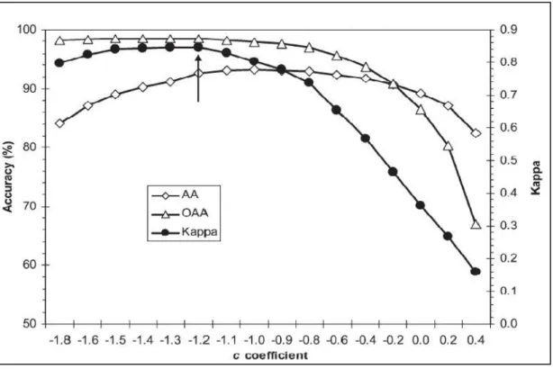
The c refers to a range of coefficient (values between -1.8 and 0.4) that can be used to calculate different thresholds to show the best change/no change (Figure

(41)

Kappa or other accuracy indices (Pu et al., 2008). However, due to the lack of

ground-truth data, the threshold values were determined by visually inspecting

maps that were produced using different coefficients. The visual inspection reveals

that as c increases (small negative value) a lot of noise is introduced but information is lost as the value of c decreases (larger negative value). Hence, the optimum threshold values is found to be in the range of -0.6 and -0.2.

Figure 4.2.1.1. Range of optimal c value. Source: Pu et al. (2008)

4.2.2. Image Classification

The next step in the image processing phase is image classification. Two types of

classification algorithms were employed, Maximum Likelihood (MLC) and Isodata

Cluster. The MLC is an algorithm that quantitatively classifies pixels by evaluating

both the variance and covariance of the categorical spectral response pattern

(Lillesand et al., 2004). This is based on the assumption that similar features with

similar spectral signature have a normal distribution and their statistical

(42)

that the analyst defines training areas to train the algorithm, which then classify

pixels based on their likelihood to belong to the defined class (CCRS, n.d.).

Isodata cluster is a method of unsupervised classification that works by iteratively

grouping cells into a user-defined number of distinct unimodal class (ESRI, 2010).

The algorithm starts by arbitrarily assigning means (center) to cluster to which

each cell with minimum distance belong. After the first iteration, the means are

recalculated until the maximum number of iteration is reached.

The MLC was used to classify the year 2000 image which serves as reference image

for all the other images. A total of 100 samples were collected for forest, 100

samples for mixed rangeland, 100 for farmland and 50 samples for bare soil. For

built-up areas, grassland and water, 50 classes were collected for each of them.

These samples were collected by visually interpreting the 2000 image using False

and True color composites. After the classification an accuracy assessment was

performed on the classified image of 2000 using the 2001 topographic and land use

map as reference data from which samples were collected.

Congalton and Green (2008) stated that the general guideline “rule of thumb”

regarding the sample size for of an accuracy assessment is to collect 50 samples for

each class in a map that has a size of less than a million hectare and less than 12

classes. For a much larger map, they suggested 75 to 100 samples points per class

as this will ensure a balance between statistical validity and practicality (Congalton

and Green, 2008, p.75). Hence, in this study, a total of 700 points were randomly

collected from the image for the purpose of an accuracy assessment. This one time

accuracy assessment is necessary not only because it is a fundamental requirement

in a change detection study but also because the 2000 map serves as the reference

(43)

For all the other images, the unsupervised classification with ISO Cluster algorithm

was employed by assigning 30 classes. The clusters of pixels were then grouped

based on the defined land use/cover categories. Interpretation of RGB images by

False Color Composite (FCC) and True Color Composite (TCC) from each

observation date was performed to assist in the assignment of the classes.

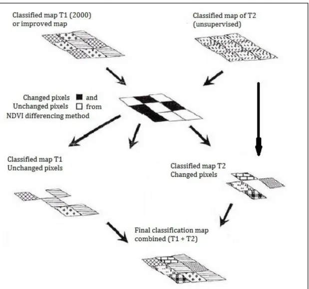
The final classification maps were obtained by combining change/no change maps

generated by NDVI differencing and maps generated from both supervised and

unsupervised classification (see Figure 4.2.2). Afterwards, a 3 x 3 pixels majority

filter was applied to all the classified maps to remove some of the speckled pattern

(noise) of individual pixels.

(44)

Figure 4.2.2. Derivation of final classification maps for five acquisition dates (1972, 1987, 1996, 2005 and 2005) by combining change/no change maps and classified maps from supervised and unsupervised methods

4.2.3. Change rationality test

To improve the final classification maps, it is necessary to understand whether or

not some of the changes between pixels make sense. For instance, it is unlikely that

built-up areas will change into forested land or farmland. Additionally, in tropical

region such as East Timor, where deforestation occurs due primarily to shifting

cultivation and expansion of farmland, change from farmland or bare soil to forest

(45)

changes between pixels. The following four rules have been used to perform this

assessment.

Let x be the number of detected categorical changes over six monitoring dates (1972–2011).

where = means no change at all, and = means that the pixel of the cover type

has undergone changes through every detection period. Consider also that = a

specific cover type and = a different cover type and T1 – T6 refers to six

observation dates.

Rule I: no change (x = 0), if a pixel is classified as the same land cover type

throughout the six monitoring periods then it is ‘correctly’ classified.

T1 T2 T3 T4 T5 T6

Correct for all cover types.

Rule II: One-time change (x = 1), if a pixel changes from one cover type to a different cover type for once, and once only, then it is classified as correct.

However, there is an exception to pixels with cover type built-up area, bare soil and

farmland. If a pixel is found to have changed from built-up area to different cover

type, it is considered as a ‘reverse’ case and is classified as ‘incorrect’. In that case,

the pixel failed Rule II and needs to be passed to the next test. Similarly, a change

of pixel with cover type farmland or bare soil to forest is also considered ‘incorrect.’

Correct; incorrect if = built-up areas

Correct; incorrect if = farmland / bare soil,

(46)

Rule III: ‘The ruleof majority’, a pixel is considered majority class if it is classified

as the same cover type for four times or more, irrespective of their order in

between T1 and T6. This pixel is considered correct and the other two pixels that

are incorrect will be reclassified similar to the correct one.

= majority class

will be reclassified as

Rule IV: this rule deals with all the pixels that failed all the previous tests above

(x > 2). Pixels in this category are those that change multiple times between cover

types but don’t retain majority. For example, a pixel in 1972 may be classified as

forest, but grassland in 1987 and built-up in 2000. It is difficult to know whether or

not this is a true land cover change and so they are considered ‘fuzzy’ pixels. Pixels

in this category will be reclassified based on the information from 2000 image

because this is the only reliable map.

4.3. Post-classification change detection

After the final maps are reclassified and improved through change rationality test, a

post-classification comparison is performed to detect LULC change. This technique

performs change detection in which comparison is made between independently

classified images (Singh, 1989). Post classification comparison has the advantage to

provide direct information on the nature of land cover change. To perform the

change detection two maps were paired to calculate their categorical change. For

instance, the map of 1972 was paired with 1987 to calculate how much of an area

of a class in 1972 map had changed in the map of 1987. This procedure was

(47)

CHAPTER 5

RESULTS AND DISCUSSION

5.1.NDVI

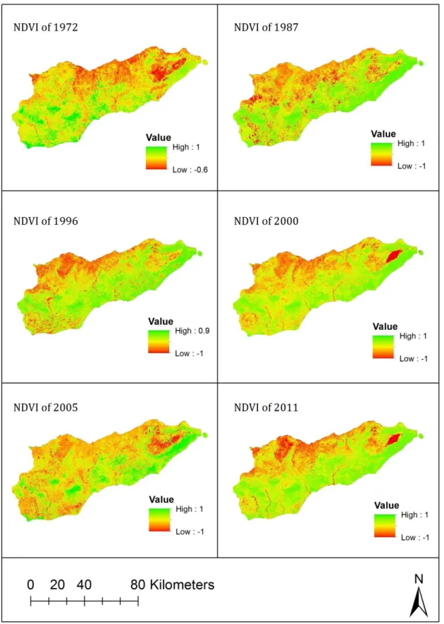
The NDVI calculations were obtained for all the observation dates (Figure 5.1.1). Visual analysis of the images shows that large proportions of healthy vegetation were located mostly in southern region of the study area. Toward the northern region, NDVI shows relatively low values. In 1972, however, high NDVI values were observed primarily in the western part of the study area. This is contrary to the distribution of vegetation in 1987 where higher NDVI values shifted toward the eastern part of the island. Although from 1996 on, the INDVI map looks fairly similar, it’s apparent that the 2005 map shows less greenness compared to all other maps. See Appendix D for enlarged version of NDVI images.

5.2.NDVI Differencing

The results from NDVI differencing techniques were obtained for all the observation dates. After conducting visual inspection of NDVI differencing images with different c coefficients, the optimal threshold values for change/no change were determined. The change/no change map were generated using the optimum threshold values ranging from -0.6 to 0.2 (see Appendix A for change/no change maps). Table 5.2.1 shows the mean, standard deviation, and optimum threshold values for all the image pairs

NDVI

Differencing

Index Decrease Index Increase Optimum

c value

Threshold

Mean SD Mean SD Decrease Increase

1972 – 1987 -0.662 0.323 -0.057 0.155 - 0.6 0.4682 0.036

1972 – 1996 0.001 0.187 0.456 0.291 -0.2 -0.0384 0.5142

1996 – 2000 -0.021 0.180 0.253 0.210 -0.2 -0.057 0.295

2000 – 2005 -0.569 0.197 -0.192 0.177 -0.6 -0.6872 -0.0858

2005 – 2011 0.142 0.176 0.547 0.200 -0.6 0.034 0.667

(48)

(49)

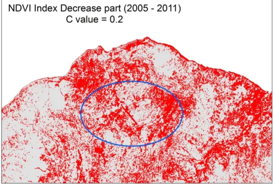
5.3. Selection of coefficients

Ideally, selection of the optimum threshold value is done by measuring its performance against some accuracy indices. However, due to the lack of ground data (reference data) in this study the selection of the optimum threshold value were done by visual inspection of each map generated using all the different c values. One of the techniques used in this study is by observing features in the image that is assumed to have a constant low (or high) index value throughout the study period and using it as a basis for helping in determining the threshold value. For instance, feature such as airport rarely changes for long period of time and so the difference value for pixels around this area should be close to zero either above or below the mean. The c values for both the index decrease and increase parts were arbitrarily chosen so that they don’t include pixels that contain the feature’s information (Figure 5.3.1). Pixels of other features, assumed to have relatively constant zero value, were also used as indicators. Hence, the threshold values were selected by distinguishing true change (larger negative value) from noise (lower negative value).

(50)

Figure 5.3.2. NDVI index decrease part shows minimum noise due to selection of low c value (larger negative).

(51)

5.4. Image classification

Conducting an accuracy assessment for a classified image is necessary especially if

the image is to be used for further analysis. It is particularly important in

post-classification change detection analysis where the accuracy of the final change

image depends on the accuracy of the independently classified images (Yuan et al.,

2005). In determining the accuracy of this image, 700 sample points were

randomly distributed across the study area. The different land use/cover

categories in the classified image were compared with the topographic map and

land use map of East Timor for the year of 2000 by using the confusion matrix. The

result shows an overall accuracy of 0.82% with a kappa index of 0.77 (Table 5.3.1).

As mentioned in the methodology section, after conducting accuracy assessment,

the 2000 map was used to classify images from other years for which NDVI

differencing identified as no change. For pixels that NDVI differencing identified as

change, they were classified using unsupervised method. Finally, these maps were

improved by applying change rationality test.

Categories Producer accuracy

(%) User accuracy (%)

Forest 90 82

Mixed Rangeland 83 86

Grassland 83 84

Farmland 74 82

Settlement 52 57

Bare soil 78 73

Water 86 86

Table 5.3.1. One time accuracy assessment for 2000 image

5.4.1. Change rationality test: Rule I

The change rationality test over the six-time multi-temporal image classification

(52)

assessment of the LULC change rationality by separating change and no change

pixels throughout the six observation dates. First it identifies pixels that don’t change and labels them as ‘correctly’ classified, and ‘uncertain’ for pixels that

change. Of the total 5572060 pixels, 3072292 pixels remained unchanged

throughout the six observation dates, accounting for 55% of the total pixels (Table

5.4.1.1). From these unchanged pixels, forest constitutes 1095588 number of

pixels, about 20% of the total, and mixed rangeland constitutes around 33%. All

other cover types together only make up about 2% of the total pixels (Figure

5.4.1.1)

Forest Mixed

Rangeland Grassland Farmland Built-up Bare soil Water Unchanged

Pixels 1095588 1856754 99048 15578 1356 3272 696

Table 5.4.1.1. Total number of unchanged pixels for each category as defined by Rule I