A segmented wavelet inspired neural network approach to compress images

(1)

A SEGMENTED WAVELET INSPIRED

NEURAL NETWORK APPROACH TO

COMPRESS IMAGES

Rekha M.Tech Scholar

Department of Computer Sc. & Engineering GITM, Gurgaon, Haryana, India

Sangeeta Yogi Assistant Professor

Geeta Assistant Professor

Abstract- The great growth in the use of internet and mobile communication devices has revolutionised the way human beings communicate and make information exchange. The necessity of efficient digital information in those devices is essential. With the advancement of technology we need more data transfer. This requires large bandwidth. Data compression is the process of converting an input data stream (the source stream) into another data stream (the output, the bit-stream, or the compressed stream) that has smaller size. Image compression is the application of data compression on digital images. It is the art and science of reducing the amount of data required to represent an image. The purpose for image compression is to reduce the amount of data required for representing sampled digital images and therefore reduce the cost for storage and transmission. Image compression plays a key role in many important applications, including image database, image communications, remote sensing. In this present work we are providing an approach to perform the image compression using improved neural network approach. Here the improvement is being done using wavelet. In this proposed system we achieve the image compression with better visibility. The system is good even for the low resolution images. In this work we work on bit area and maintain the information of the bits. Because of this as we decompress the image first the decode process is performed to get the bit information and then image restoration is applied to get back the clear visual image. We have applied the work on no. of sample images of different types. We also compared the image quality using MSE and PSNR.

I. INTRODUCTION

The great growth in the use of internet and mobile communication devices has revolutionized the way human beings communicate and make information exchange. The necessity of efficient digital information in those devices is

(2)

essential. With the advancement of technology we need more data transfer. This requires large bandwidth. Data compression is the process of converting an input data stream (the source stream) into another data stream (the output, the bit-stream, or the compressed stream) that has smaller size. Image compression is the application of data compression on digital images. It is the art and science of reducing the amount of data required to represent an image.

1.1 Three Main Reasons:-why present multimedia systems require that data must be compressed: a) Large storage requirements of multimedia data

b) Relatively slow storage devices that do not allow playing multimedia data (especially video) in real-time, and

c) The present network bandwidth, which does not allow real-time video data transmission.

1.2 Ways To Evaluate The Quality Of Compressed Images:- There are three major ways to evaluate the quality of compressed images: SNR, Subjective Rating (SR), and Diagnostic Accuracy (DA). Evaluation of a particular compression scheme also includes compression efficiency (CE) and compression complexity (CC). For judging loss compression methods, all of the five metrics - SNR, SR, DA, CE and CC can be used. However for lossless compression, the comparison can be made solely on the basis of CE and CC.

1.3 Challenges

a) Developing real time compression algorithm

b) Guaranteed quality of service in case of multimedia applications

c) Cost minimization, because cost and time cost of transmission and storage tend to be directly proportional to the volume of data.

1.4 Error Matrices:- that are used to compare the various image compression techniques. They are Mean Square Error (MSE) and the Peak Signal-to-Noise Ratio (PSNR). The MSE is the cumulative squared error between the compressed and the original image whereas PSNR is the measure of the peak error.

The quality of image coding is typically assessed by the Peak signal-to-noise ratio (PSNR) defined as

PSNR = 20 log 10[255/sqrt(MSE)]

OBJECTIVE

a) To achieve high PSNR and low MSE.

b) To get better compression ratio by different epochs. c) To train the network by using different activation functions.

d) To achieve high accuracy and generalizing ability for approximating the problems.

II.IMAGE COMPRESSION USING BACK PROPAGATION

The back propagation technique described by Rumelhart et al was a very significant development in the field of neural networks, and has found many applications in a wide range of areas of research. The application of a simple three-layer back propagation network for image data compression was first proposed by Cottrell et al. and subsequently studied and developed by others [2,3]. Some inherent features of back propagation network image data compression schemes are: (a) the network structure is massively parallel, (b) the network is adaptive, (c) the network determines the compressed features of the original image in a self organizing manner during the training stage, and

(3)

(d) the intrinsic generalization property of the structure enables it to process images outside the training set (novel images) effectively [1].

In this section, we briefly review the basic idea of using a back propagation network to achieve image compression. A number of researchers have shown that multilayer preceptor networks are able to learn a transform for reducing signal redundancy, and are capable of learning a reverse transform to recover the information (with some degradation) from a more compact (compressed) form of representation. The network shown in Fig. 1 has N input nodes, H hidden layer nodes (H<N) andNoutput nodes.

The input to the network, X , is a vector of dimension N,and in our application, Xis an mxn

( N =mxn) block of pixels extracted from an image. The sum of the inputs, sh(i),

for node i in the hidden layer is calculated as where wh(j,i) is the connection weight from jth input node to the ith

node in the hidden layer, x(j)is the jth input element (pixel value), and bh(i) is the bias input of the ith hidden layer

node.

Similarly, the sum of the inputs to the ith output node is calculated as

Figure 1: Back Propagation based Compression Approach

(4)

wherewo(j,i) is the connection weight from the jth hidden layer node to the ith output node, b,(i) is the bias input to

the ith output node, and h(j) is the output of the jth hidden layer node. A sigmoid function defined by equation (1) is applied to sh(i) and so(i) to obtain the output value of the node for the hidden and output layers respectively[1].

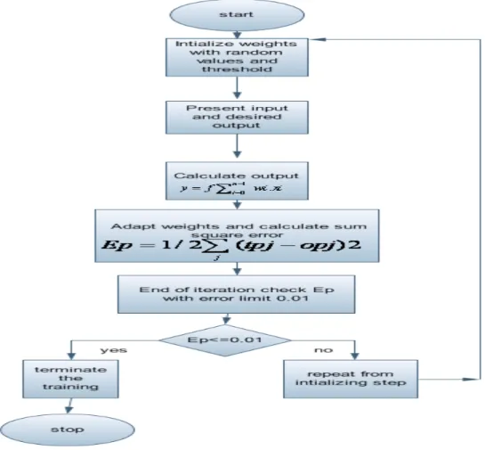
III. PROPOSED WORK

A two layer Back Propagation neural network and the Wavelet decomposition algorithm were considered. Image coding using a feed forward neural network consists of the following steps:

An image, F, is divided into rxc blocks of pixels. Each block is then scanned to form a input vector x (n) of size p=rxc

It is assumed that the hidden layer of the layer network consists of L neurons each with P synapses, and it is characterized by an appropriately selected weight matrix Wh.

All N blocks of the original image is passed through the hidden layer to obtain the hidden signals, h(n), which represent encoded input image blocks, x(n) If L<P such coding delivers image compression.

It is assumed that the output layer consists of m=p=rxc neurons, each with L synapses. Let Wy be an appropriately

selected output weight matrix. All N hidden vector h(n), representing an encoded image H, are passed through the output layer to obtain the output signal, y(n). The output signals are reassembled into p=rxc image blocks to obtain a reconstructed image, Fr.

Once the weight matrices have been appropriately selected, any image can be quickly encoded using the Wh

matrix, and then decoded (reconstructed) using the Wy matrix.

The DWT is one of the fundamental processes in the JPEG2000 image compression algorithm [2]. The DWT is a transform which can map a block of data in the spatial domain into the frequency domain. The DWT returns information about the localized frequencies in the data set. A two-dimensional (2D) DWT is used for images. The 2D DWT decomposes an image into four blocks, the approximation coefficients and three detail coefficients. The details include the horizontal, vertical, and diagonal coefficients. The lower frequency (approximation) portion of the image can be preserved, while the higher frequency portions may be approximated more loosely without much visible quality loss. The DWT can be applied once to the image and then again to the coefficients which the first DWT produced. It can be visualized as an inverted treelike structure. The original image sits at the top. The first level DWT decomposes the image into four parts or branches, as previously mentioned. Each of those four parts can then have the DWT applied to them individually, splitting each into four distinct parts or branches [3].

Concisely, ANNs are basically a collection of massively interconnected nodes or commonly known as processing elements (PE) or nodes. Before the network can be used, the weights connecting two nodes need to be adjusted first. This alteration of weights also known as training is done by going through the network a set of input and output pairs (a complete set is known as an epoch). The weights are fine tune accordingly based on one of the many available training algorithms which are pertinent to the network configuration.

One of the most popular training algorithms available for example is the back propagation method. In this method, the weights are updated based on the error between the input and output pairs. This training process above will be iterated until a certain condition set by the network designer is met. Among the criterion normally implemented is the mean square error of the network or the gradient of the error function. Through this training, the network would then be able to generalize any unseen before inputs [4].

(5)

Modification is made to a standard JPEG2000 algorithm by substituting the quantization block with a backward propagation ANN. In this proposed work standard JPEG2000 quantizes the transformed coefficients using a preset quantization matrix and then round up. After multiplying with the quantization matrix, most of the higher frequencies that are localized on the bottom right comer will be rounded up to zero. Finally, the remaining will be quantized and compression thus achieved due to the loss of higher frequency information. On the other hand, the modified algorithm will make use of the BP to store all the coefficients in the synaptic weights after the learning process. The inputs feed into the network would be the spatial coordinate of the image while the outputs will be the corresponding coefficients.

3.1 Algorithm

The proposed compression algorithm is given as

1. Divide the image in image segments of some normalized size like mxm

2. Normalize the pixel value.

3. Perform the Wavelet Transformation to reduce the error.

4. Train the sub images using 3 layer back propagation Network.

5. Pass the input to the input layer,

6. From this input values some output is driven for the hidden layer and after applying some weightage the output values are derived.

7. Calculate the MSE.

8. Update weight and re perform the process.

9. Map the pixel of image with neighboring pixels

10. Calculate the compression ratio

3.2 Mat lab Function

net = newff(PR,[S1 S2...SNl],{TF1 TF2...TFNl},BTF,BLF,PF)

3.2.1Description

net = newff creates a new network with a dialog box.

newff(PR,[S1 S2...SNl],{TF1 TF2...TFNl},BTF,BLF,PF) takes,

PR -- R x 2 matrix of min and max values for R input elements

Si -- Size of ith layer, for Nl layers

TFi -- Transfer function of ith layer, default = 'tansig'

BTF -- Back propagation network training function, default = 'traingdx'

BLF -- Back propagation weight/bias learning function, default = 'learngdm'

PF -- Performance function, default = 'mse'

[net,tr,Y,E,Pf,Af] = train(net,P,T,Pi,Ai,VV,TV)

(6)

3.2.2 Description

train trains a network net according to net.trainFcn and net.trainParam.

train (NET,P,T,Pi,Ai,VV,TV) takes,

net -- Neural Network

P -- Network inputs

T -- Network targets, default = zeros

Pi -- Initial input delay conditions, default = zeros

Ai -- Initial layer delay conditions, default = zeros

VV -- Structure of validation vectors, default = []

IV. TOOLS USED IN SIMULATOR

Toolbox used in MATLAB for our proposed work is Image Processing Toolbox.

Image Processing Toolbox™ provides a comprehensive set of reference-standard algorithms and graphical tools for image processing, analysis, visualization, and algorithm development. You can perform image enhancement, image deblurring, feature detection, noise reduction, image segmentation, spatial transformations, and image registration. Many functions in the toolbox are multithreaded to take advantage of multicore and multiprocessor computers.

Image Processing Toolbox supports a diverse set of image types, including high dynamic range, gigapixel resolution, ICC-compliant color, and tomography images. Graphical tools let you explore an image, examine a region of pixels, adjust the contrast, create contours or histograms, and manipulate regions of interest (ROIs). With the toolbox algorithms you can restore degraded images, detect and measure features, analyze shapes and textures, and adjust the color balance of images.

4.1 Simulation Results:

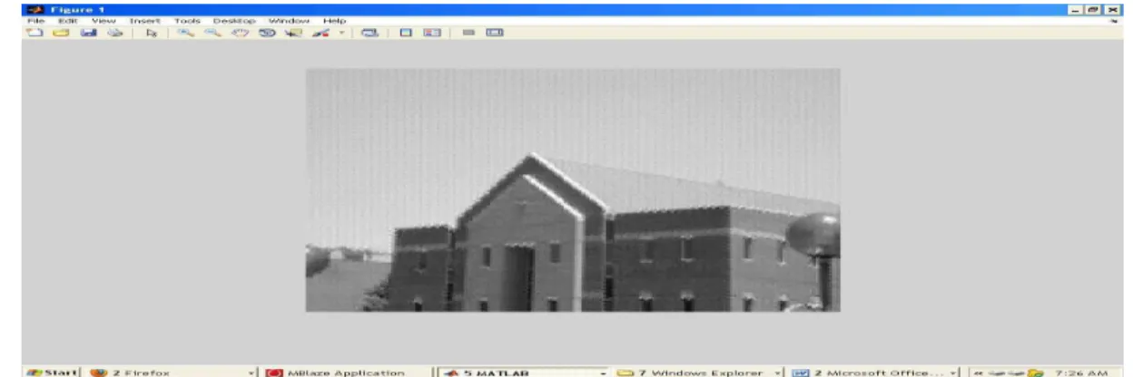
Image : 12.jpg

Image Format : JPEG

Image Size :7.96 KB

Resolution : 256x256

Figure 2: Input Image

(7)

Figure 2 is showing the input image of size 256x256, in jpg format. It is the actual image that we have to compress using Wavelet based neural network approach.

Figure 3: Neural Training process for compression

As we can see in figure 2 the training process using neural network is shown. The process is to perform the image compression. As we can see process is run for 10 epochs and the goal is set at .0001. The goal is achieved after 5 epochs.

In figure 3, the performance graph obtained from the neural network is shown. In this graph it shows the achievement of goal after some defined epochs. The dark blue line is sowing the actual performance.

Figure 4: Performance Graph

(8)

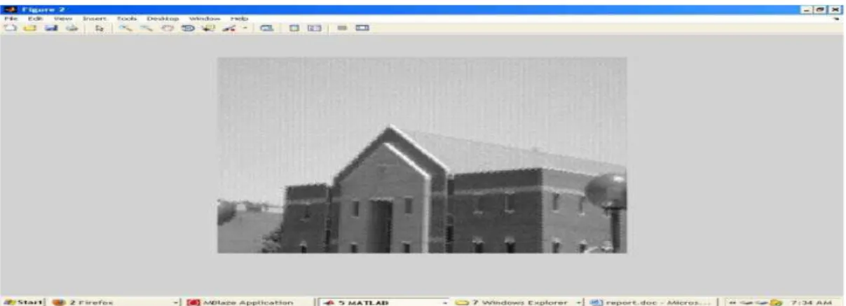
Figure 5: Result Compressed Image

In figure the result is shown for input image. As we can see the result image is not losing its quality. The obtained image is compressed with given statistics

Image Size : 6.59 kb

Compression Ratio : 82%

Type : Lossy Compression

PSNR Value : 30.25

Figure 6: Recovered Image

Figure 6 is showing the results of the recovered image after performing the neural network approach on compressed image. As the compression type is lossy some information is lost during the recovery process. The obtained image is of size 7.24

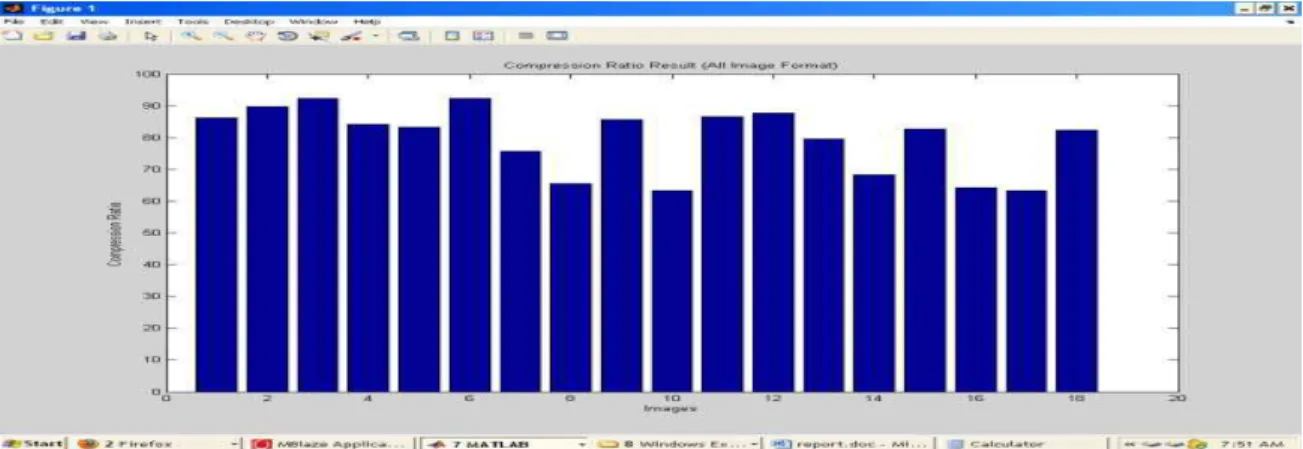
4.2 Analysis

We have tested the complete work on different kind of images of different size and different file formats. The obtained results are taken in the form of time taken, PSNR ratio and the compression ratio.

(9)

Figure 7: Compression Ratio Results

Figure 7 is showing the results obtained in terms of compression ratio. As we can see the minimum compression obtained is around 65% and the maximum ratio is about 93%.

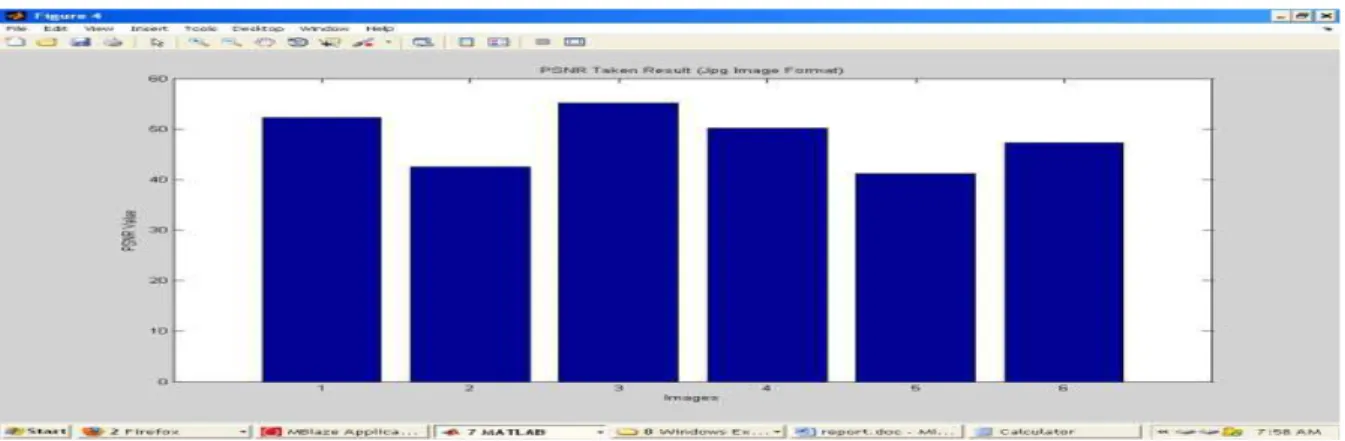
Figure 8: PSNR Ratio Results

Figure 8 is showing the results obtained in terms of PSNR ratio on different kind of images. As we can see the minimum psnr values obtained is around 35 and the maximum ratio is about 47. The results are taken on jpg , bmp and tiff images.

Figure 9: Time Results

(10)

Figure 9 is showing the results obtained in terms of Time taken to compress on different kind of images. As we can see the minimum psnr values obtained is around 70 and the maximum ratio is about 475. The results are taken on jpg , bmp and tiff images.

Figure 10: PSNR Ratio Results

Figure 10 is showing the results obtained in terms of PSNR ratio on different kind of images. As we can see the minimum psnr values obtained is around 40 and the maximum ratio is about 55. The results are taken on jpg , bmp and tiff images.

Figure 11 : Time Results

Figure 11 is showing the results obtained in terms of Time Taken on different kind of images. As we can see the minimum time values obtained is around 60 and the maximum ratio is about 150. The results are taken on jpg , bmp and tiff images.

V. CONCLUSION AND FUTURE SCOPE

5.1 Conclusion

In this proposed system we achieve the image compression with better visibility. The system is good even for the

low resolution images. In this work we work on bit area and maintain the information of the bits. Because of this as

we decompress the image first the decode process is performed to get the bit information and then image restoration

(11)

is applied to get back the clear visual image. We have applied the work on no. of sample images of different types.

We also compared the image quality using MSE and PSNR. We can conclude that the system will provide the better

visibility after the image restoration.

5.2 Future Work

In this proposed system we worked on simple jpg, bmp, png and tiff images. We can enhance this work for the

images of medical areas such as dicom images or the pgm images. We can also enhance this work for the moving

image i.e. videos and animated gif etc.

VI. REFERENCE

[2] Stefan Craciun,et al. “Wireless Transmission of Neural Signals Using Entropy and Mutual Information Compression”, IEEE

[3] LI Huifang,et al. “A New Method of Image Compression Based On Quantum Neural Network”, 2010 International Conference of

[4] Aditya V. Padaki,et al. “Improving Performance in Neural Network Based Pulse Compression for Binary and Polyphase Codes”,12th International Conference on Computer Modelling and Simulation 978-0-7695-4016-0/10© 2010 IEEE,2010

[6] Jin Wang,at al. “ ECG Data Compression Research Based on Wavelet Neural Network”,International Conference on Computer,

[9] Vilas Gaidhane,et al. “Image Compression using PCA and Improved Technique with MLP Neural Network”,International Conference on Advances in Recent Technologies in Communication and Computing 978-0-7695-4201-0/10© 2010 IEEE, 2010.

[10] GUO Hui,et al. “Wavelet packet and neural network basis medical image compression”,978-1-4244-7161-4/10©2010 IEEE,2010. [11] Wen-Nung Lie,at al. “A Perceptually Lossless Image Compression Scheme Based On Jnd Refinement By Neural Network,”Fourth

[13] T. Martinetz and K. Schulten,et al. “ A neural gas learns topologies”. In T. Kohonen, K. M¨akisara, O. Simula, and J. Kangas, editors, Artificial Neural Networks, pages 397–402. North-Holland, Amsterdam, 1991.

[14] J. D. Murray, W. Vanryper, and D. Russell,et al. “Encyclopedia of Graphics File Formats”, O’Reilly UK, Cambridge, 1996. [15] W. B. Pennebaker and J. L. Mitchell,et al. “ JPEG: Still Image Data Compression Standard”, Kluwer International, Dordrecht, 1992.