Use of portable FTIR spectrometers for detecting greenhouse gas emissions of the megacity Berlin – Part 1: Instrumental line shape characterisation and calibration of a quintuple of spectrometers

(1)

AMTD

8, 2735–2766, 2015

Greenhouse gas emissions of Berlin –

Part 1: Instrumental calibration of spectrometers

M. Frey et al.

Title Page

Abstract Introduction

Conclusions References

Tables Figures

◭ ◮

Back Close

Full Screen / Esc

Printer-friendly Version

Interactive Discussion

Discussion

P

a

per

|

Discussion

P

a

per

|

Discussion

P

a

per

|

Discussion

P

a

per

|

Atmos. Meas. Tech. Discuss., 8, 2735–2766, 2015 www.atmos-meas-tech-discuss.net/8/2735/2015/ doi:10.5194/amtd-8-2735-2015

This discussion paper is/has been under review for the journal Atmospheric Measurement Techniques (AMT). Please refer to the corresponding final paper in AMT if available.

Use of portable FTIR spectrometers for

detecting greenhouse gas emissions of

the megacity Berlin – Part 1: Instrumental

line shape characterisation and

calibration of a quintuple of

spectrometers

M. Frey1, F. Hase1, T. Blumenstock1, J. Groß1, M. Kiel1, G. Mengistu Tsidu1,3, K. Schäfer2, M. Kumar Sha1, and J. Orphal1

1

Karlsruhe Institute of Technology (KIT), Institute for Meteorology and Climate Research (IMK-ASF), Karlsruhe, Germany

2

Karlsruhe Institute of Technology (KIT), Institute for Meteorology and Climate Research (IMK-IFU), Garmisch-Partenkirchen, Germany

3

(2)

AMTD

8, 2735–2766, 2015

M. Frey et al.

Title Page

Tables Figures

◭ ◮

Back Close

Full Screen / Esc

Discussion

P

a

per

|

Discussion

P

a

per

|

Discussion

P

a

per

|

Discussion

P

a

per

|

Received: 24 February 2015 – Accepted: 26 February 2015 – Published: 13 March 2015

Correspondence to: M. Frey ([email protected])

(3)

AMTD

8, 2735–2766, 2015

M. Frey et al.

Title Page

Tables Figures

◭ ◮

Back Close

Full Screen / Esc

Discussion

P

a

per

|

Discussion

P

a

per

|

Discussion

P

a

per

|

Discussion

P

a

per

|

Abstract

Several low resolution spectrometers were used to investigate the CO2and CH4

emis-sions of the megacity Berlin. Before and after the campaign the instruments were tested side-by-side. An excellent level of agreement and stability was found between the di_ff er-ent spectrometers: the drifts inXCO2andXCH4are within 0.005 and 0.035 %,

respec-5

tively. The instrumental line shape characteristics of all spectrometers were found to be close to nominal. Cross-calibration factors forXCH₄ and XCO₂ were established for each spectrometer. An empirical airmass correction factor has been applied. As a last calibration step, using a co-located TCCON spectrometer as a reference, a common factor has been derived for the low-resolution campaign spectrometers, which ensures 10

that the records are compatible to the WMO in-situ scale. Finally as a first result of the Berlin campaign we show the excellent agreement of ground pressure values obtained from total column measurements and in situ records.

1 Introduction

The continuing increase of atmospheric greenhouse gas abundances is the major 15

driver of anthropogenic global warming. Accurate measurements of the variable atmo-spheric concentrations are required for the quantification of sinks and sources of these gases (Olsen and Randerson, 2004). In the last years great efforts have been under-taken to measure column-averaged dry air mole fractions of greenhouse gases with global coverage. Examples are satellite-borne instruments like SCIAMACHY (Franken-20

berg et al., 2006), GOSAT (Morino et al., 2011) or the recently launched OCO-2 sensor (Frankenberg et al., 2015). For the validation of OCO-2, a network of ground based high resolution Fourier-transform infrared (FTIR) spectrometers of the type 125HR from Bruker has been initiated by Caltech: the Total Carbon Column Observation Net-work (TCCON). Currently, about 23 TCCON globally distributed stations measure the 25

(4)

AMTD

8, 2735–2766, 2015

M. Frey et al.

Title Page

Tables Figures

◭ ◮

Back Close

Full Screen / Esc

Discussion

P

a

per

|

Discussion

P

a

per

|

Discussion

P

a

per

|

Discussion

P

a

per

|

solar absorption spectra in the near infrared (NIR) (Wunch et al., 2010). TCCON has been carefully calibrated against in situ aircraft measurements and sets the reference for remote-sensing measurements of column-averaged greenhouse gas observations. However, it is difficult to use this technical approach for the observation of sources and sinks on a regional scale, because the laboratory spectrometers applied for TC-5

CON are not portable. Recently, KIT developed in cooperation with Bruker, Ettlingen, a portable low resolution FTIR spectrometer for the observation of greenhouse gases in the NIR and demonstrated the excellent stability of the device (Gisi et al., 2012). The spectrometer is now available from Bruker under the part name EM27/SUN. This leightweight device has low infrastructure demands so it can be operated on a cam-10

paign basis, at remote places and even on mobile platforms as ships (Klappenbach, 2015). These features not only enable the EM27/SUN to contribute to the total column measurements of the TCCON in previously underrepresented regions, in particular it can be used to gain additional information about isolated sinks and sources of green-house gases. Boundary layer abundances of greengreen-house gases influenced by emis-15

sions from cities have been observed since long using mass spectroscopy (von der Weiden-Reinmüller et al., 2014) or cavity ring down techniques (Newman et al., 2013). The downside of this approach is the high sensitivity to local sources which overem-phasizes the near vicinity and the sensitivity with respect to assumptions on vertical exchange of air masses. Here we demonstrate another approach to measure the emis-20

sions of a mega city. For this purpose, we operated five EM27/SUN spectrometer sur-rounding the Berlin conurbation. Over a period of three weeks, we measured the total column of CO₂, CH₄, H₂O and O₂ at the di_fferent stations. As the emission of Berlin is small compared to the atmospheric background signal, in the sub percentage order, high precision and stability of the instrument are a prerequisite. This kind of method 25

(5)

AMTD

8, 2735–2766, 2015

M. Frey et al.

Title Page

Tables Figures

◭ ◮

Back Close

Full Screen / Esc

Discussion

P

a

per

|

Discussion

P

a

per

|

Discussion

P

a

per

|

Discussion

P

a

per

|

of water vapour signatures for the determination of instrumental line shape (ILS) char-acteristics. Moreover, we tested the participating instruments side-by-side for several days before and after the campaign, determined the level of instrumental stability and deduced calibration factors forXCH₄andXCO₂in order to assure that data measured by different spectrometers are compatible between each other and with TCCON mea-5

surements.

2 Instrumentation and spectrometer characteristics

2.1 EM 27 SUN spectrometer

For the acquisition of solar spectra we utilize the Bruker EM27/SUN which was devel-oped in collaboration with the KIT. A detailed description of the spectrometer can be 10

found in Gisi et al. (2012), in the following only a short overview including changes from the original setup is given.

The EM27/SUN features a RockSolidTMpendulum interferometer with two cube cor-ner mirrors and a CaF2beamsplitter. This setup achieves high stability against thermal

influences and vibrations. Gimbal-mounted retroreflectors move a geometrical distance 15

of 0.45 cm leading to an optical path difference (OPD) of 1.8 cm which corresponds to a spectral resolution of 0.5 cm−1. As a minor modification of the prototype spec-trometer described by Gisi et al. (2012), the production device contains an off-axis mirror with a focal length of 127 mm for centering the solar beam on the detector. To-gether with the field stop (0.6 mm diameter) this leads to a semi Field-of-View (FOV) 20

of 2.36 mrad. Measurements are recorded with an InGaAs detector operated at ambi-ent temperature. Due to an electronics update it is now possible to record double-sided interferograms (IFG) of 0.5 cm−1resolution. The detector is a photodiode type G12181-010K from Hamamatsu with a size of 1 mm×1 mm and spectral coverage from 5000

to 11 000 cm−1

. In contrast to the detector used in the prototype that operated in the 25

(6)

AMTD

8, 2735–2766, 2015

M. Frey et al.

Title Page

Tables Figures

◭ ◮

Back Close

Full Screen / Esc

Discussion

P

a

per

|

Discussion

P

a

per

|

Discussion

P

a

per

|

Discussion

P

a

per

|

observation of CH₄. In addition, total columns of O₂, CO₂ and H₂O are derived from the recorded spectra. The detector signal is DC coupled and thereby supports the cor-rection of variable atmospheric transmission (Keppel-Aleks et al., 2007).

2.2 Ghost to parent ratio

The EM 27 records spectra in the region from 100 to 15 798 cm−1_{, so in order to satisfy}

5

the Nyquist theorem the sampling of the IFG has to be performed at every zerocrossing of the laser signal (HeNe laser, wavelength 633 nm). If the signal is not taken at exactly zero intensity, systematic sampling errors are introduced leading to artefacts in the measured spectrum, so called sampling ghosts (Messerschmidt et al., 2010; Dohe et al., 2013). Bruker recently released an effective workaround for this problem which 10

we adopted for our measurements. A temporal linear interpolation is applied for locating the downward zero crossings. This method suppresses the ghosts below the detection limit (<5×10−6). In addition, we tested this set up for possible line shape errors and

other kinds of out-of-band artefacts, but found no detrimental effects.

2.3 Intrumental line shape 15

Precise knowledge of a spectrometer’s instrumental line shape (ILS) is of utmost im-portance to gain correct information from measurements as using wrong ILS values leads to systematic errors in the gas retrieval. The ILS can be divided into two parts. One part describes the modulation loss through inherent self-apodization of the spec-trometer which is present also in an ideal instrument. This contribution can easily be 20

calculated utilizing the OPD and FOV of the spectrometer. The other component of the ILS results from misalignments and optical aberrations of the spectrometer and can be characterised by a modulation efficiency amplitude and a phase error, both func-tions of the OPD (Hase et al., 1999). These parameters have to be deduced from lab measurements.

(7)

AMTD

8, 2735–2766, 2015

M. Frey et al.

Title Page

Tables Figures

◭ ◮

Back Close

Full Screen / Esc

Discussion

P

a

per

|

Discussion

P

a

per

|

Discussion

P

a

per

|

Discussion

P

a

per

|

For the TCCON spectrometer, the standard procedure to derive the ILS are gas cell measurements. In contrast, we determine the ILS by measuring several meters of lab air and evaluating the water vapor lines in the spectral region between 7000 and 7400 cm−1. As light source a collimated standard 50 W halogen light bulb is used. With this approach no gas cell is necessary, which is advantageous for measurement 5

campaigns. For the analysis of the measured data we use version 14 of the retrieval software LINEFIT (Hase et al., 1999). In LINEFIT one can choose between a simple and extended ILS model. As the ILS characteristics were close to nominal, we used the simple two-parameter ILS model. For the H2Olinelist we use the HITRAN 2009 linelist

with minor adjustments, see Sect. 4.1. Needed parameters are ground pressure, ambi-10

ent temperature and the distance between spectrometer and light source. Temperature and pressure were recorded using the MHB-382SD data logger with a temperature ac-curacy of±0.8◦C and pressure accuracy of±3 hPa (above 1000 hPa) or±2 hPa (below

1000 hPa). A typical fit result is shown in Fig. 1. The SD of the residual is very low, 1σ=0.24 %.

15

We measured the ILS for the different spectrometers before and after the Berlin campaign. The resulting ILS values are presented in Table 1. For the trace gas re-trieval we use the mean value of the measurements before and after the campaign, the setup for these experiments was exactly the same. One can see that the values show very good agreement. The correlation between modulation e_fficiency amplitude 20

and XCO2 was deduced from a sensitivity study and is in agreement with Gisi et al.

(2012). Intrument 2 has the biggest difference in terms of ILS modulation efficiency be-fore and after the campaign with 0.24 %, corresponding to a change of only 0.04 % for the column-averaged dry-air mole fraction (DMF) of carbon dioxide,XCO2. Note that

this is not self-evident since the instruments were transported from Karlsruhe to Berlin 25

(8)

AMTD

8, 2735–2766, 2015

M. Frey et al.

Title Page

Tables Figures

◭ ◮

Back Close

Full Screen / Esc

Discussion

P

a

per

|

Discussion

P

a

per

|

Discussion

P

a

per

|

Discussion

P

a

per

|

3 Measurement sites and data acquisition

In order to measure during the campaign small differences upstream and downstream of a source, a instrument to instrument consistency is of utmost importance for this setup. For this purpose, calibration measurements were carried out.

3.1 Calibration measurements at KIT Campus North 5

The calibration measurements were performed before the Berlin campaign on three sunny days between 6 June and 16 June and after the campaign on three consecutive days 16–18 July on top of our o_ffice building north of Karlsruhe, with an altitude of 133 m a.s.l., coordinates are 49.094◦N and 8.434◦E. The spectrometers were moved from the lab on the fourth floor to the roof terrace on the seventh floor thus being ex-10

posed to mechanical stress. Then they were coarsely oriented north, without e_ffort for levelling. If further orientation was needed, we manually moved the spectrometer so that the solar beam was centered onto the entrance window. The CamTracker pro-gram was then able to track the sun. As we operated the EM27/SUN in summer, it was heated up to temperatures above 40◦C. In order to protect the electronics from the 15

heat, we built a sun cover for the EM27/SUN, which considerably reduced the temper-atures inside the spectrometer. We recorded double-sided interferograms with 0.5 cm−1

resolution. With 10 scans and a scanner velocity of 10 kHz, one measurement takes about 58 s.

For precise time recording, we used a GPS Receiver. Additionally on-site pressure 20

and temperature profiles are available from tall tower meteorological measurements.

3.2 Berlin campaign measurements

(9)

AMTD

8, 2735–2766, 2015

M. Frey et al.

Title Page

Tables Figures

◭ ◮

Back Close

Full Screen / Esc

Discussion

P

a

per

|

Discussion

P

a

per

|

Discussion

P

a

per

|

Discussion

P

a

per

|

so that CO₂emissions really can be attributed to Berlin. Thirdly, the flat topography is favorable, which supports the interpretation of the recorded data.

During the campaign period 23 June–11 July measurements were performed at five different stations around Berlin, four of them roughly located on a circle with a radius of 12 km around the city centre of Berlin. One instrument was positioned inside the 5

Berlin motorway ring in Charlottenburg, closer to the city centre than the other instru-ments. A map with the different sites is shown in Fig. 2. The coordinates and altitudes of the different stations are displayed in Table 2. At the sites, temperature and pressure profiles were recorded using the MHB-382SD data logger. To obtain comparable data, we measured a long time series in Karlsruhe to determine calibration factors between 10

the di_fferent loggers. The data was used to calculate the exact altitude of the stations. The records of ground pressure were also used in the creation of the model atmo-sphere. The measurement procedures (scan speed, resolution, numerical apodisation, etc.) applied during the campaign were identical to those applied for the calibration measurements.

15

4 Data analysis

4.1 Data processing

In a first step, the recorded interferograms are Fourier transformed using the Norton-Beer-Medium apodisation function. This apodisation is useful for reducing sibelobes around the spectral lines, an undesired feature in unapodised low resolution spec-20

tra, which would complicate the further analysis. Furthermore, a DC-correction is per-formed. Together with a quality filter, which discards IFGs with intensity fluctuations above 10 % and intensities below 10 % of the maximal modulation amplitude, this is implemented in a Python tool. In this work, we analyzed spectra utilizing the PROFFIT Version 9.6. This code is in wide use and has been thoroughly tested in the past, e.g. 25

(10)

AMTD

8, 2735–2766, 2015

M. Frey et al.

Title Page

Tables Figures

◭ ◮

Back Close

Full Screen / Esc

Discussion

P

a

per

|

Discussion

P

a

per

|

Discussion

P

a

per

|

Discussion

P

a

per

|

the low resolution of the EM27/SUN, we fitted the atmospheric spectra by scaling of a-priori trace gas profiles. As source of the a-priori profiles, we utilized the WACCM ver. 6 climatology (http://www2.cesm.ucar.edu/working-groups/wawg).

For the retrieval we need accurate temperature and pressure profiles. In case of the Karlsruhe calibration experiments we use on-site data together with MERRA model 5

data, which provides temperature and pressure data on a 1.25◦×1.25◦grid from 1000

to 0.1 hPa 8 times a day. For the Berlin campaign we utilize local meteorological ra-diosonde data and the NCEP model to set up the temperature profiles. We take the NCEP data as the starting values and apply a linear ascent during the day, which is the temperature difference between the 12 a.m. and 6 p.m. sonde data, for the first height 10

levels (until an altitude of approximately 4 km). For the height levels above 4 km we take the unaltered NCEP data, as the change during the day is negligible. For the pressure profiles we use the time series of the logger data, scale the values to 30 m a.s.l. and take the smoothed mean of the di_fferent stations pressure data. We calculate the pres-sure of the different altitude levels from the barometric height formula using a scaling 15

height of 8.7 km.

Every retrieval is dependent on proper spectroscopic parameters for the solar lines and atmospheric gases absorption lines. We use the HITRAN 2008 line list in its origi-nal form for CH4, the HITRAN 2008 linelist with a line-mixing parameterisation for CO2

adopted from a code provided by Hartmann (Lamouroux et al., 2010) and the linelist 20

used by TCCON for O2. For the H2O linelist we use the HITRAN 2009 linelist with

changes used by (Wunch et al., 2010) and additional ad hoc adjustments where it seemed appropriate.

4.2 Spectral windows

For the evaluation of the O2 gas column we use the 7765–8005 cm− 1

spectral region, 25

which is also applied in the TCCON analysis (Wunch et al., 2010). For CO2 we

(11)

AMTD

8, 2735–2766, 2015

M. Frey et al.

Title Page

Tables Figures

◭ ◮

Back Close

Full Screen / Esc

Discussion

P

a

per

|

Discussion

P

a

per

|

Discussion

P

a

per

|

Discussion

P

a

per

|

to 6390 cm−1. CH4 is evaluated in the 5897–6145 cm− 1

spectral domain. For H2O the

8353 to 8463 cm−1region is used.

An example fit for the different spectral windows is shown in Fig. 3. The residuum of the spectral fit for the water column retrieval is much bigger than for the other gases. Due to the large variability of water vapor in the atmosphere, larger linelist errors are 5

expected. Overall the fit quality is very good withσ=0.2 % for CO₂and CH₄,σ=0.1 % for O2andσ=0.5 % for H2O.

5 Results calibration measurements

In this section we present results of the calibration measurements performed before and after the Berlin campaign. First we show the uncalibrated total columns followed by 10

column-averaged DMFXGas of carbon dioxide and methane, whereXGas is defined as

XGas=GasColumn

O_2Column ·0.2095 (1)

To make the measurements comparable to WMO scale, in TCCON the standard pro-cedure is to divide the calculated DMFs by a calibration factor (Wunch et al., 2010). We 15

also apply this post processing in our work. ForXCO₂ the factor is 0.9898 whereas it is 0.9765 forXCH4.

5.1 Total column amounts

In Fig. 4 are depicted the column values of the measured species of the different in-struments. From first glance, it is clear that the shape of all the spectrometers is nearly 20

(12)

AMTD

8, 2735–2766, 2015

M. Frey et al.

Title Page

Tables Figures

◭ ◮

Back Close

Full Screen / Esc

Discussion

P

a

per

|

Discussion

P

a

per

|

Discussion

P

a

per

|

Discussion

P

a

per

|

well as on two days after the Berlin campaign and therefore was only partly able to per-form measurements. Intraday changes of the O2column can be attributed to pressure

changes for the largest part, which will be shown in Sect. 6. There are slight system-atic offsets, strongest between Instrument 2 and Instrument 4 with a difference of 0.2 %. However, note that a similar offset is also observed in the CO2and CH4gas columns,

5

as can be seen in Fig. 4, therefore the resulting effects on the target quantitiesXCO2

andXCH₄are much smaller.

For a better comparison an intercalibration factor between the instruments is established. This is done in the following way. We take the separate measurement days and divide the data into smaller bins of 15 min duration. Inside each bin we take 10

the mean value of all measurements from all stations and minimize the residuum for all stations. In Table 3 the calibration factors for the O2 column for the calibration

measurements before and after the campaign are given. Differences before and after the campaign are very small, only 0.04 % for Instrument 2 and 4 and even less for the other instruments. This is suprisingly good, because column values are sensitive to 15

various potential error sources, including ILS errors, timing errors, tracking errors and nonlinearities. For further analysis we use the dry air mole fraction of the gases, which are less prone to errors, because these tend to cancel out in the rationing of columns, see Eq. (1).

20

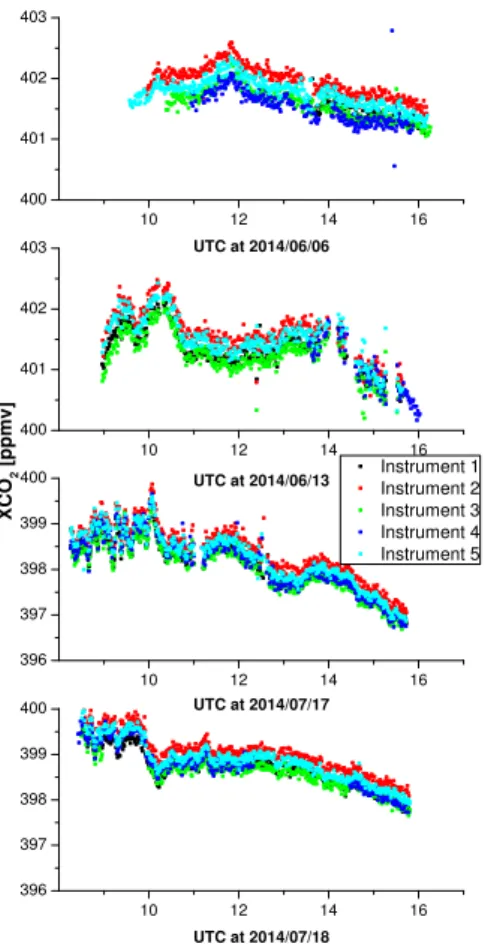
5.2 Column-averaged dry air mole fraction

Figure 5 shows the column-averaged DMF of CO2, which was calculated using Eq. (1).

In this representation systematic errors tend to cancel out, which leads to a high degree of reproducibility in the time series di_fference between the instruments. Until this point, no post calibration has been performed, only the individual ILS of each instrument has 25

been taken into account.

(13)

col-AMTD

8, 2735–2766, 2015

M. Frey et al.

Title Page

Tables Figures

◭ ◮

Back Close

Full Screen / Esc

Discussion

P

a

per

|

Discussion

P

a

per

|

Discussion

P

a

per

|

Discussion

P

a

per

|

umn calibration. For XCO₂ we obtain a perfect agreement. The difference is below 0.005 % or 0.02 ppm for all instruments. This means we can apply a global intercali-bration factor which is valid before and after the campaign. This is an important pre-requisite for campaign measurements. ForXCH₄the agreement is slightly worse with 0.035 %, but still very good. In Fig. 6 the calibratedXCH4time series for the calibration

5

measurements is depicted. Note that one global intercalibration factor is applied for all measurement days.

The scatter is very low for both species. Variations during the day stem from real signals, for example theXCO2 peaks on the sixteenth of July were also measured by

a co-located TCCON instrument (see Fig. 7). 10

5.3 Solar zenith angle dependency

There is a slight solar zenith angle (SZA) dependency in theXCO2 and XCH4 data,

which is hard to see in Figs. 5 and 6 because the SZA is low during the day in summer. Also it is superimposed to the actual diurnal cycle. In order to make the data compatible with the WMO reference scale, it is nevertheless important to correct for a systematic 15

airmass dependency originating from spectroscopic uncertainties and approximations by the radiative transfer model. For this we use a method similar to that proposed by (Wunch et al., 2010). The correction formula is

XGasc=XGasunc

( 1+a

"

θ+b

90◦₊_b

2

−

45◦+b 90◦₊_b

2#)

wherea,bare fit parameters,θis the SZA,XGascandXGasunc are the airmass

de-20

(14)

AMTD

8, 2735–2766, 2015

M. Frey et al.

Title Page

Tables Figures

◭ ◮

Back Close

Full Screen / Esc

Discussion

P

a

per

|

Discussion

P

a

per

|

Discussion

P

a

per

|

Discussion

P

a

per

|

tained from a comprehensive evaluation of EM27/SUN data from a ship cruise (Klap-penbach, 2015). This data is not influenced by local source contributions and clearly shows the SZA dependency in the XCO2 and XCH4 data. It turned out that the O2

column-averaged mole fraction does not show a detectable SZA dependence for SZA <80◦; the SZA dependence is essentially generated by the CO2 and CH4 mole

frac-5

tions in the numerator. The obtained parameters are a=6.296×10−3,b=1.291 for

XCO2 and a=3.796×10− 3

, b=16.04 for XCH4. Using this correction we receive

data comparable to in situ scale measurements, supported by the comparison with a collocated TCCON spectrometer. Figure 7 shows the airmass dependency corrected XCO2values together with TCCON DMF for 16 July. Additionally an in situ scaling was

10

performed to match the EM27/SUN values to the TCCON instrument. This factor of 0.99505 was determined with the method described in Sect. 5.1. The EM27/Sun val-ues match the TCCON valval-ues remarkably well. Again one global factor was found valid for the measurements before and after the campaign.

Figure 8 showsXCH4values for the same day. Similar toXCO2the values between

15

EM27/SUN spectrometers and TCCON instrument differ slightly towards evening. For the in situ scaling factor we obtain 0.99511.

6 Berlin campaign

At the end of the first part of this study, we present the O₂columns as recorded at all sites during the Berlin campaign. In order to compare this dataset with in situ pressure 20

values derived from the MHB-382SD data loggers, we calculate the ground pressure from the measured O₂and H₂O total columns:

P_S=O_2Column÷0.2095×µ¯+H2OColumn×µH₂O

×g×exp

−∆h

hS

(2)

PSis the surface pressure, ¯µthe molecular mass of dry air,µH₂Othe molecular mass

(15)

AMTD

8, 2735–2766, 2015

M. Frey et al.

Title Page

Tables Figures

◭ ◮

Back Close

Full Screen / Esc

Discussion

P

a

per

|

Discussion

P

a

per

|

Discussion

P

a

per

|

Discussion

P

a

per

|

the chosen reference altitude of 30 m a.s.l. and h_S the scaling height. For the sake of comparison, all pressure values derived from the spectra are transformed to this common reference altitude. We observe a systematic offset between these records and the actual ground pressure of 3.0 %. This discrepancy can mainly be attributed to oxygen line intensity errors (Washenfelder et al., 2006). In Fig. 9 we scaled the pressure 5

values obtained from the total columns to the in situ data for better comparability. The variability of the slope of the in situ measurements is nicely reproduced by the column data.

7 Conclusions

We developed a calibration procedure for mobile FTIR spectrometers which we applied 10

to 5 spectrometers used for observing greenhouse gas emissions from Berlin during a field campaign during June and July 2014. We were successful in demonstrating the high degree of consistency. Between the instruments we established cross-calibration factors which were found valid before and after the field campaign. Drifts were below 0.005 % for XCO2 and 0.035 % for XCH4. In addition a method for deriving ILS

pa-15

rameters from open path measurements is described and was used for showing that the ILS is close to nominal for all instruments. Changes in the ILS before and after the campaign were very small, within 0.24 % modulation efficiency amplitude at maximum optical path difference. Furthermore an empirical airmass correction was applied to compensate for a spurious SZA dependency of the data. As a last calibration step the 20

in situ calibration factor derived by a comparison with a co-located TCCON instrument was applied. The same empirical calibration factor of 0.9951±0.0001 was found valid

for bothXCO₂andXCH₄in order to make results comparable to WMO scale.

Finally we displayed ground pressures calculated from oxygen and water vapor columns at all sites during the Berlin campaign. The excellent station-to-station con-25

(16)

AMTD

8, 2735–2766, 2015

M. Frey et al.

Title Page

Tables Figures

◭ ◮

Back Close

Full Screen / Esc

Discussion

P

a

per

|

Discussion

P

a

per

|

Discussion

P

a

per

|

Discussion

P

a

per

|

In conclusion, we are highly confident that these portable spectrometers are very useful instruments for observing local sinks and sources of carbon dioxide and methane. In part two of this work (Hase et al., 2015), we will present the greenhouse gas observations themselves and compare these data with predictions of a simple dis-persion model.

5

Acknowledgements. We acknowledge support by the ACROSS research infrastructure of the Helmholtz Association.

We acknowledge Friedrich Klappenbach from the “Institute for Meteorology and Climate Re-search – Atmospheric Trace Gases and Remote Sensing (IMK-ASF)” at the KIT for providing the fit parameters used for the correction of the SZA dependency.

10

We acknowledge Stephan Kraut from the “Institute for Meteorology and Climate Research – Troposphere Research (IMK-TRO)” at the KIT for providing tall-tower meteorological data.

We acknowledge the Global Modelling and Assimilation Office (GMAO) and the GES DISC for the dissemination of Merra meteorological datasets.

We acknowledge Michael Gisi and Gregor Surawicz from Bruker for their invaluable support

15

in bringing the EM27/SUN spectrometers into service.

The article processing charges for this open-access publication have been covered by a Research Centre of the Helmholtz Association.

References 20

Dohe, S., Sherlock, V., Hase, F., Gisi, M., Robinson, J., Sepúlveda, E., Schneider, M., and Blu-menstock, T.: A method to correct sampling ghosts in historic near-infrared Fourier transform spectrometer (FTS) measurements, Atmos. Meas. Tech., 6, 1981–1992, doi:10.5194/amt-6-1981-2013, 2013. 2740

Frankenberg, C., Meirink, J. F., Bergamaschi, P., Goede, A. P. H., Heimann, M., Körner, S.,

25

(17)

AMTD

8, 2735–2766, 2015

M. Frey et al.

Title Page

Tables Figures

◭ ◮

Back Close

Full Screen / Esc

Discussion

P

a

per

|

Discussion

P

a

per

|

Discussion

P

a

per

|

Discussion

P

a

per

|

Frankenberg, C., Pollock, R., Lee, R. A. M., Rosenberg, R., Blavier, J.-F., Crisp, D., O’Dell, C. W., Osterman, G. B., Roehl, C., Wennberg, P. O., and Wunch, D.: The Orbiting Carbon Obser-vatory (OCO-2): spectrometer performance evaluation using pre-launch direct sun measure-ments, Atmos. Meas. Tech., 8, 301–313, doi:10.5194/amt-8-301-2015, 2015. 2737

Gisi, M., Hase, F., Dohe, S., Blumenstock, T., Simon, A., and Keens, A.: XCO₂-measurements

5

with a tabletop FTS using solar absorption spectroscopy, Atmos. Meas. Tech., 5, 2969–2980, doi:10.5194/amt-5-2969-2012, 2012. 2738, 2739, 2741

Hase, F., Blumenstock, T., and Paton-Walsh, C.: Analysis of the instrumental line shape of high-resolution Fourier transform IR spectrometers with gas cell measurements and new retrieval software, Appl. Optics, 38, 3417–3422, doi:10.1364/AO.38.003417, 1999. 2740, 2741

10

Hase, F., Frey, M., Blumenstock, T., Groß, J., Kiel, M., Kohlhepp, R., Mengistu Tsidu, G., Schäfer, K., Sha, M. K., and Orphal, J.: Use of portable FTIR spectrometers for detecting greenhouse gas emissions of the megacity Berlin – Part 2: Observed time series ofXCO₂ and XCH₄, Atmos. Meas. Tech. Discuss., 8, 2767–2791, doi:10.5194/amtd-8-2767-2015, 2015. 2750

15

Keppel-Aleks, G., Toon, G. C., Wennberg, P. O., and Deutscher, N. M.: Reducing the impact of source brightness fluctuations on spectra obtained by Fourier-transform spectrometry, Appl. Optics, 46, 4774–4779, doi:10.1364/AO.46.004774, 2007. 2740

Klappenbach, F.: Observations ofXCO₂on the Polarstern cruise 2014, in preparation, 2015. 2738, 2748

20

Lamouroux, J., Tran, H., Laraia, A., Gamache, R., Rothman, L., Gordon, I., and Hartmann, J.-M.: Updated database plus software for line-mixing in CO₂ infrared spectra and their test using laboratory spectra in the 1.5–2.3 µm region, J. Quant. Spect. Radiat. T., 111, 2321– 2331, doi:10.1016/j.jqsrt.2010.03.006, 2010. 2744

Mellqvist, J., Samuelsson, J., Johansson, J., Rivera, C., Lefer, B., Alvarez, S., and Jolly, J.:

25

Measurements of industrial emissions of alkenes in Texas using the solar occultation flux method, J. Geophys. Res.-Atmos., 115, D00F17, doi:10.1029/2008JD011682, 2010. 2738 Messerschmidt, J., Macatangay, R., Notholt, J., Petri, C., Warneke, T., and Weinzierl, C.: Side

by side measurements of CO₂by ground-based Fourier transform spectrometry (FTS), Tellus B, 62, 749–758, doi:10.1111/j.1600-0889.2010.00491.x, 2010. 2740

30

(18)

AMTD

8, 2735–2766, 2015

M. Frey et al.

Title Page

Tables Figures

◭ ◮

Back Close

Full Screen / Esc

Discussion

P

a

per

|

Discussion

P

a

per

|

Discussion

P

a

per

|

Discussion

P

a

per

|

Preliminary validation of column-averaged volume mixing ratios of carbon dioxide and methane retrieved from GOSAT short-wavelength infrared spectra, Atmos. Meas. Tech., 4, 1061–1076, doi:10.5194/amt-4-1061-2011, 2011. 2737

Newman, S., Jeong, S., Fischer, M. L., Xu, X., Haman, C. L., Lefer, B., Alvarez, S., Rap-penglueck, B., Kort, E. A., Andrews, A. E., Peischl, J., Gurney, K. R., Miller, C. E., and

5

Yung, Y. L.: Diurnal tracking of anthropogenic CO₂ emissions in the Los Angeles basin megacity during spring 2010, Atmos. Chem. Phys., 13, 4359–4372, doi:10.5194/acp-13-4359-2013, 2013. 2738

Olsen, S. C. and Randerson, J. T.: Differences between surface and column atmospheric CO2 and implications for carbon cycle research, J. Geophys. Res.-Atmos., 109, D02301,

10

doi:10.1029/2003JD003968, 2004. 2737

Schneider, M. and Hase, F.: Ground-based FTIR water vapour profile analyses, Atmos. Meas. Tech., 2, 609–619, doi:10.5194/amt-2-609-2009, 2009. 2743

Schneider, M., Sepúlveda, E., García, O., Hase, F., and Blumenstock, T.: Remote sensing of water vapour profiles in the framework of the Total Carbon Column Observing Network

(TC-15

CON), Atmos. Meas. Tech., 3, 1785–1795, doi:10.5194/amt-3-1785-2010, 2010. 2743 Seppúlveda, E., Schneider, M., Hase, F., García, O. E., Gomez-Pelaez, A., Dohe, S.,

Blumen-stock, T., and Guerra, J. C.: Long-term validation of tropospheric column-averaged CH₄mole fractions obtained by mid-infrared ground-based FTIR spectrometry, Atmos. Meas. Tech., 5, 1425–1441, doi:10.5194/amt-5-1425-2012, 2012. 2743

20

von der Weiden-Reinmüller, S.-L., Drewnick, F., Zhang, Q. J., Freutel, F., Beekmann, M., and Borrmann, S.: Megacity emission plume characteristics in summer and winter investigated by mobile aerosol and trace gas measurements: the Paris metropolitan area, Atmos. Chem. Phys., 14, 12931–12950, doi:10.5194/acp-14-12931-2014, 2014. 2738

Washenfelder, R. A., Toon, G. C., Blavier, J.-F., Yang, Z., Allen, N. T., Wennberg, P. O., Vay, S.

25

A., Matross, D. M., and Daube, B. C.: Carbon dioxide column abundances at the Wisconsin Tall Tower site, J. Geophys. Res.-Atmos., 111, D22305, doi:10.1029/2006JD007154, 2006. 2749

Wunch, D., Toon, G. C., Wennberg, P. O., Wofsy, S. C., Stephens, B. B., Fischer, M. L., Uchino, O., Abshire, J. B., Bernath, P., Biraud, S. C., Blavier, J.-F. L., Boone, C.,

Bow-30

(19)

AMTD

8, 2735–2766, 2015

M. Frey et al.

Title Page

Tables Figures

◭ ◮

Back Close

Full Screen / Esc

Discussion

P

a

per

|

Discussion

P

a

per

|

Discussion

P

a

per

|

Discussion

P

a

per

|

(20)

AMTD

8, 2735–2766, 2015

M. Frey et al.

Title Page

Tables Figures

◭ ◮

Back Close

Full Screen / Esc

Discussion

P

a

per

|

Discussion

P

a

per

|

Discussion

P

a

per

|

Discussion

P

a

per

|

Table 1.Compilation of ILS modulation efficiencies before and after the measurement cam-paign.

Instr. 3 Jun 15 Jul

(21)

AMTD

8, 2735–2766, 2015

M. Frey et al.

Title Page

Tables Figures

◭ ◮

Back Close

Full Screen / Esc

Discussion

P

a

per

|

Discussion

P

a

per

|

Discussion

P

a

per

|

Discussion

P

a

per

|

Table 2.Coordinates and altitude of the Berlin measurement stations.

Site Long. (◦_E) _{Lat. (}◦_N) _{Altit. (m a.s.l.)}

Mahlsdorf 13.589 52.486 39.0

Charlottenburg 13.302 52.505 47.7

Heiligensee 13.228 52.622 34.5

Lindenberg 13.519 52.601 63.3

(22)

AMTD

8, 2735–2766, 2015

M. Frey et al.

Title Page

Tables Figures

◭ ◮

Back Close

Full Screen / Esc

Discussion

P

a

per

|

Discussion

P

a

per

|

Discussion

P

a

per

|

Discussion

P

a

per

|

Table 3.Calibration factors for O₂column before and after the campaign for the different instru-ments. Instrument 1 has been scaled to one, which is an arbitrary choice.

Instr. O₂col. before O₂col. after

1 1.00000 1.00000

2 1.00010 0.99970

3 1.00037 1.00015

4 1.00236 1.00196

(23)

AMTD

8, 2735–2766, 2015

M. Frey et al.

Title Page

Tables Figures

◭ ◮

Back Close

Full Screen / Esc

Discussion

P

a

per

|

Discussion

P

a

per

|

Discussion

P

a

per

|

Discussion

P

a

per

|

Table 4.Calibration factor forXCO₂ andXCH₄for the different instruments before and after the campaign.

Instr. XCO₂bef. XCO₂aft. XCH₄bef. XCH₄aft.

1 1.00000 1.00000 1.00000 1.00000

2 0.99924 0.99921 0.99927 0.99940

3 1.00015 1.00016 0.99971 0.99962

4 0.99987 0.99987 0.99856 0.99882

(24)

AMTD

8, 2735–2766, 2015

M. Frey et al.

Title Page

Tables Figures

◭ ◮

Back Close

Full Screen / Esc

Discussion

P

a

per

|

Discussion

P

a

per

|

Discussion

P

a

per

|

Discussion

P

a

per

|

7000 7100 7200 7300 7400

-0,2 0,0 0,2 0,4 0,6 0,8 1,0

T

ra

n

s

m

is

s

io

n

Wavenumber [cm-1]

Measurement EM27 Fit

Residuum * 10

(25)

AMTD

8, 2735–2766, 2015

M. Frey et al.

Title Page

Tables Figures

◭ ◮

Back Close

Full Screen / Esc

Discussion

P

a

per

|

Discussion

P

a

per

|

Discussion

P

a

per

|

Discussion

P

a

per

|

(26)

AMTD

8, 2735–2766, 2015

M. Frey et al.

Title Page

Tables Figures

◭ ◮

Back Close

Full Screen / Esc

Discussion

P

a

per

|

Discussion

P

a

per

|

Discussion

P

a

per

|

Discussion

P

a

per

|

7800 7850 7900 7950 8000

0,0 0,2 0,4 0,6

6200 6250 6300 6350

0,0 0,2 0,4 0,6 0,8 1,0

5900 5950 6000 6050 6100

0,0 0,2 0,4 0,6 0,8 1,0

8400 8450

-0,2 0,0 0,2 0,4 0,6 0,8

Measurement EM 27 Fit

Residuum * 10 Measurement EM 27 Fit

Residuum * 20 Measurement EM 27 Fit

Residuum * 20

O

2

T

ra

n

sm

issi

o

n

CO₂

CH₄

Wavenumber [cm-1_]

H₂O

(27)

AMTD

8, 2735–2766, 2015

M. Frey et al.

Title Page Abstract Introduction Conclusions References Tables Figures ◭ ◮ ◭ ◮ Back Close

Full Screen / Esc

Printer-friendly Version Interactive Discussion Discussion P a per | Discussion P a per | Discussion P a per | Discussion P a per |

10 12 14 16 4.54

4.56 4.58

10 12 14 16 8.62 8.64 8.66 8.68 8.70 8.72 8.74

10 12 14 16 3.82

3.84 3.86 3.88 3.90

10 12 14 16 4.56

4.58 4.60

10 12 14 16 8.62 8.64 8.66 8.68 8.70 8.72 8.74

10 12 14 16 3.82

3.84 3.86 3.88 3.90

10 12 14 16 4.56

4.58 4.60

10 12 14 16 8.56 8.58 8.60 8.62 8.64 8.66 8.68 8.70

10 12 14 16 3.82

3.84 3.86 3.88 3.90

10 12 14 16 4.56

4.58 4.60

10 12 14 16 8.56 8.58 8.60 8.62 8.64 8.66

10 12 14 16 3.82 3.84 3.86 3.88 3.90 [1025

molec. / m2 ]

UTC at 2014/07/18 UTC at 2014/07/17 UTC at 2014/06/13 UTC at 2014/06/06

[1023 molec. / m2

] [1028_{molec. / m}2_]

Instrument 1 Instrument 2 Instrument 3 Instrument 4 Instrument 5

O2 - Column CO2 - Column CH4 - Column

(28)

AMTD

8, 2735–2766, 2015

M. Frey et al.

Title Page

Tables Figures

◭ ◮

Back Close

Full Screen / Esc

Discussion

P

a

per

|

Discussion

P

a

per

|

Discussion

P

a

per

|

Discussion

P

a

per

|

10 12 14 16

400 401 402 403

10 12 14 16

400 401 402 403

10 12 14 16

396 397 398 399 400

10 12 14 16

396 397 398 399 400

UTC at 2014/06/06

X

C

O2

[

p

m

v

]

UTC at 2014/06/13

UTC at 2014/07/17

UTC at 2014/07/18

(29)

AMTD

8, 2735–2766, 2015

M. Frey et al.

Title Page

Tables Figures

◭ ◮

Back Close

Full Screen / Esc

Discussion

P

a

per

|

Discussion

P

a

per

|

Discussion

P

a

per

|

Discussion

P

a

per

|

10 12 14 16

1.790 1.795 1.800 1.805 1.810 1.815

10 12 14 16

1.790 1.795 1.800 1.805 1.810 1.815

10 12 14 16

1.790 1.795 1.800 1.805 1.810 1.815

10 12 14 16

1.790 1.795 1.800 1.805 1.810 1.815

UTC at 2014/06/06

X

C

H4

[

p

m

v

]

UTC at 2014/06/13

UTC at 2014/07/17

UTC at 2014/07/18

(30)

AMTD

8, 2735–2766, 2015

M. Frey et al.

Title Page

Tables Figures

◭ ◮

Back Close

Full Screen / Esc

Discussion

P

a

per

|

Discussion

P

a

per

|

Discussion

P

a

per

|

Discussion

P

a

per

|

10

12

14

16

18

393

394

395

396

397

_{Instrument 1}

Instrument 2 Instrument 3 Instrument 4 Instrument 5

TCCON Instrument

X

C

O

2

[

p

m

v

]

UTC at 2014/07/16

(31)

AMTD

8, 2735–2766, 2015

M. Frey et al.

Title Page

Tables Figures

◭ ◮

Back Close

Full Screen / Esc

Discussion

P

a

per

|

Discussion

P

a

per

|

Discussion

P

a

per

|

Discussion

P

a

per

|

10 12 14 16 18

1.790 1.795 1.800 1.805 1.810 1.815 1.820 1.825

1.830 Instrument 1

Instrument 2 Instrument 3 Instrument 4 Instrument 5 TCCON Instrument

X

C

H

4

[

p

m

v

]

UTC at 2014/07/16

(32)

AMTD

8, 2735–2766, 2015

M. Frey et al.

Title Page

Tables Figures

◭ ◮

Back Close

Full Screen / Esc

Discussion

P

a

per

|

Discussion

P

a

per

|

Discussion

P

a

per

|

Discussion

P

a

per

|

26.06.2014 30.06.2014 04.07.2014 08.07.2014 995

1000 1005 1010 1015 1020

1025 Mahlsdorf * In situ factor Charlottenburg * In situ factor Heiligensee * In situ factor Lindenberg * In situ factor Lichtenrade * In situ factor In situ (PT Logger data)