Evaluation of CALIOP 532 nm aerosol optical depth over opaque water clouds

www.atmos-chem-phys.net/15/1265/2015/ doi:10.5194/acp-15-1265-2015

© Author(s) 2015. CC Attribution 3.0 License.

Evaluation of CALIOP 532 nm aerosol optical depth over opaque

water clouds

Z. Liu1,2, D. Winker2, A. Omar2, M. Vaughan2, J. Kar1,2, C. Trepte2, Y. Hu2, and G. Schuster2

1_{Science Systems and Applications, Inc., Hampton, Virginia, USA} 2_{NASA Langley Research Center, Hampton, Virginia, USA} Correspondence to:Z. Liu (zhaoyan.liu@nasa.gov)

Received: 11 August 2014 – Published in Atmos. Chem. Phys. Discuss.: 12 September 2014 Revised: 19 December 2014 – Accepted: 28 December 2014 – Published: 5 February 2015

Abstract. With its height-resolved measurements and near global coverage, the CALIOP lidar onboard the CALIPSO satellite offers a new capability for aerosol retrievals in cloudy skies. Validation of these retrievals is difficult, how-ever, as independent, collocated and co-temporal data sets are generally not available. In this paper, we evaluate CALIOP aerosol products above opaque water clouds by applying multiple retrieval techniques to CALIOP Level 1 profile data and comparing the results. This approach allows us to both characterize the accuracy of the CALIOP above-cloud aerosol optical depth (AOD) and develop an error budget that quantifies the relative contributions of different error sources. We focus on two spatial domains: the African dust trans-port pathway over the tropical North Atlantic and the African smoke transport pathway over the southeastern Atlantic. Six years of CALIOP observations (2007–2012) from the north-ern hemisphere summer and early fall are analyzed. The analysis is limited to cases where aerosol layers are located above opaque water clouds so that a constrained retrieval technique can be used to directly retrieve 532 nm aerosol optical depth and lidar ratio. For the moderately dense Sa-hara dust layers detected in the CALIOP data used in this study, the mean/median values of the lidar ratios derived from a constrained opaque water cloud (OWC) technique are 45.1/44.4±8.8 sr, which are somewhat larger than the value of 40±20 sr used in the CALIOP Level 2 (L2) data products. Comparisons of CALIOP L2 AOD with the OWC-retrieved AOD reveal that for nighttime conditions the L2 AOD in the dust region is underestimated on average by∼26 % (0.183 vs. 0.247). Examination of the error sources indicates that errors in the L2 dust AOD are primarily due to using a lidar ratio that is somewhat too small. The mean/median lidar ratio

retrieved for smoke is 70.8/70.4±16.2 sr, which is consistent with the modeled value of 70±28 sr used in the CALIOP L2 retrieval. Smoke AOD is found to be underestimated, on av-erage, by∼39 % (0.191 vs. 0.311). The primary cause of AOD differences in the smoke transport region is the ten-dency of the CALIOP layer detection scheme to prematurely assign layer base altitudes and thus underestimate the geo-metric thickness of smoke layers.

1 Introduction

properties in cloudy skies. (The advent of innovative new re-trieval techniques suggests that this situation is now chang-ing for the better; e.g., see Waquet et al., 2009; Torres et al., 2012; Yu et al., 2012; Jethva et al., 2013; and Waquet et al., 2013; and an overview by Yu and Zhang, 2013). However, beginning in June 2006 a global data set of height-resolved measurements of aerosols and clouds has been continuously acquired by the Cloud-Aerosol Lidar with Orthogonal Polar-ization (CALIOP), deployed aboard the Cloud-Aerosol Lidar and Infrared Pathfinder Satellite Observations (CALIPSO) platform. These active sensor data offer a new and unique opportunity to characterize the global three-dimensional (3-D) distribution of aerosols, including aerosols located above low clouds (Winker et al., 2013). Aerosol extinction pro-files and aerosol optical depth (AOD) can be derived from the CALIOP measurements even for aerosols located over clouds or other bright surfaces. CALIOP’s ability to quantify the spatial distribution and optical properties of above-cloud aerosols represents an important step forward, as this infor-mation is required to more accurately assess aerosol intercon-tinental transport and radiative and climate impacts (Schulz et al., 2006; Chand et al., 2009; Yu et al., 2012).

CALIOP retrievals of AOD in cloud-free skies have been evaluated by comparisons with MODIS-Aqua (Kittaka et al., 2011; Redemann et al., 2012) and with AERONET (Schus-ter et al., 2012; Omar et al., 2013). Other studies have examined seasonal and regional-mean aerosol vertical dis-tributions for the purpose of model evaluation (Yu et al., 2010; Koffi et al., 2012) and noted deficiencies in the ver-tical aerosol distributions predicted by the models. Winker et al. (2013) reported an initial evaluation of the accuracy of the CALIOP Level 3 (L3, gridded, monthly mean) aerosol extinction profiles. These preliminary results showed that monthly-mean CALIOP aerosol profiles provide quantita-tive characterization of elevated aerosol layers within major transport pathways, but a more detailed validation of the trievals of these elevated aerosol layers is needed. Most re-cently, Kacenelenbogen et al. (2014) evaluated the CALIOP above-cloud aerosol retrieval, by comparing the CALIOP re-trieved AOD with the AOD measured by the NASA Langley Research Center (LaRC) airborne high-spectral-resolution li-dar (HSRL) during 86 coincident flights in North America (mostly in the US and during daytime). Their comparison showed that the CALIOP standard processing can substan-tially underestimate the occurrence frequency of aerosols when optical depths are smaller than 0.02. This study pro-vides a useful snapshot of CALIOP measurements of tenuous aerosol layers in the free troposphere.

In this paper, we refine a previously developed opaque wa-ter cloud (OWC) constrained retrieval technique (Hu et al., 2007) and introduce two variations on the standard CALIOP aerosol extinction retrieval algorithm. We then apply these retrievals to six years of nighttime CALIOP 532 nm Level 1 (L1) profile data in two regions in the Atlantic Ocean to study the optical properties of transported mineral dust and smoke

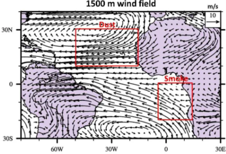
Figure 1.Spatial domains analyzed (red boxes) and wind fields

(ar-rows) from ECMWF data for July and August from 2007 to 2012. The northern region (10–30◦N, 50–15◦W) is along the Saharan dust transport pathway over the tropical North Atlantic, while the southern region (20–0◦S, 5◦W–15◦E) is along the smoke transport pathway over the tropical South Atlantic.

from biomass fires. Finally, these results are used to evaluate the quality of standard CALIOP Level 2 (L2) aerosol prod-ucts and to quantify the contributions from several potential error sources.

2 Spatial domains considered

within this region there are extensive stratocumulus decks that lie at the top of the marine boundary layer (MBL) and beneath the dust layers. When these clouds are opaque, the 532 nm cloud-integrated attenuated backscatter can be used to derive the optical depth of the overlying aerosol, which can subsequently be used to retrieve an estimate of the dust lidar ratio (i.e., the ratio of extinction to 180◦_{-backscatter,} Hu et al., 2007; Liu et al., 2008). Only the most active dust transport months of June–August are considered.

The other region selected is over the southeastern Atlantic off the west coast of southern Africa. Savanna fires are one of the largest sources of black carbon emissions to the atmo-sphere, with southern Africa being one of the major source regions (Bond et al., 2013). Southern Africa is characterized by intense biomass burning during boreal summer (June– October) (Cooke et al., 1996) and African savannas are the largest single source of biomass burning emissions (Levine et al., 1995). Extensive smoke plumes are advected westward to the southeastern Atlantic. Climate model studies have shown that the climate sensitivity to black carbon can be two or more times larger than that to carbon dioxide for a given top-of-atmosphere radiative forcing (Hansen et al., 1997; Cook and Highwood, 2004). While it is well known that biomass burning aerosols can make a significant contribution to ra-diative forcing, this contribution is poorly quantified (e.g., Chand et al., 2009). Smoke layers over the southeastern At-lantic generally overlie vast decks of stratocumulus clouds. There is no consensus among models as to even the sign of the direct aerosol forcing in this region (Schulz et al., 2006), in part due to the uncertainty in model-based estimates of the relative vertical locations of the clouds and the trans-ported smoke. Recent studies based on CALIOP observa-tions have investigated the magnitude of the aerosol radia-tive effect over this region (Chand et al., 2009; Sakaeda et al., 2011). The presence of persistent stratocumulus under-neath the smoke layer allows application of the OWC con-strained retrieval technique, thus providing an independent retrieval for comparison with the standard CALIOP products. The months considered are from July to September over the six year period (2007–2012).

3 Methodology

In this section we briefly describe the lidar inversion tech-niques and the algorithms used in CALIOP standard data processing. We also review the opaque water cloud con-strained retrieval technique (Hu et al., 2007) which we will use to directly derive the aerosol optical depths above clouds for comparison with the CALIOP standard retrievals. In ad-dition, a rescaling technique applied to the CALIOP L2 data and full-column retrievals that make direct use of the CALIOP L1 data will be used to help further assess the per-formance of the standard retrieval and to partition contribu-tions of different error sources to the AOD uncertainties.

3.1 Solutions of lidar equation

The standard CALIOP data processing retrieves aerosol ex-tinction and backscatter coefficients from the measured pro-files via a numerical solution to the lidar equation (Young and Vaughan, 2009). By assuming that the relationship be-tween aerosol extinction and backscatter remains constant within any given layer, the aerosol lidar ratio (i.e., extinction-to-backscatter ratio) is defined bySa=σ (r)/β(r), and the

solution to the lidar equation can be written as

β_a(r)= B

′_(r)

exp−2ηSaR_rr₀βa(r′)dr′

−βm(r). (1)

In this expressionB′(r)=X(r)/C/exp(−2Rr

r₀σmdr′)is the lidar return signal, normalized (i.e., recalibrated) at r0 and

corrected for molecular attenuation. X(r) is the range-corrected lidar return signal at ranger, C is a calibration coefficient determined at the calibration range r0, and σm

is the extinction coefficient due to molecular scattering and ozone absorption.β_a andβ_m are the aerosol and molecu-lar backscattering coefficients, respectively, with subscripts a and m representing the aerosol and molecular scattering, respectively.ηis the multiple scattering factor (Platt, 1973), andS_a∗=ηSais the effective lidar ratio. The molecular

scat-tering components can be determined using meteorological data from radiosonde measurements or atmospheric mod-els. In the CALIOP data processing, a global meteorologi-cal analysis product from NASA’s Global Modeling and As-similation Office (GMAO) is used to calculate the necessary molecular backscatter and extinction coefficients. For Ver-sion 3 (V3) CALIOP lidar retrievals, the data calibration at 532 nm is performed by comparing return signals from 30– 34 km altitudes with a molecular reference profile (Powell et al., 2009). Assuming thatSa andηcan be specified a priori,

the remaining unknown quantity in Eq. (1) isβ_a(r), which is present on both sides of the equation, thus necessitating an iterative numerical solution.

The aerosol lidar ratio, Sa, is a key parameter in the

li-dar inversion.Sa is an intrinsic optical property of aerosols

that varies depending on the aerosol composition, size distri-bution, and shape. OnceSa is determined, both the aerosol

backscatter coefficient, βa, and extinction, σa, can be

re-trieved. The retrieval accuracy is often dominated by uncer-tainties inSa(Young et al., 2013).

primary CALIOP L1 data products are calibrated attenuated backscatter profiles measured for each laser shot correspond-ing to a horizontal resolution of 333 m. Because of the pres-ence of some amount of stratospheric aerosols in the V3 cal-ibration region (30–34 km), the V3 L1 profiles can be biased low by a few percent (Rogers et al., 2011). To correct this, all the V3 L1 profiles were recalibrated for this paper using calibration coefficients determined at altitudes of 36–40 km (Vernier et al., 2009).

After calibration and range registration, atmospheric lay-ers are detected using a threshold technique, referred to as the selective iterative boundary locater (SIBYL), applied to profiles of 532 nm attenuated scattering ratio (Vaughan et al., 2009). Dense clouds can be detected in single-shot pro-files, while detection of aerosol layers usually requires av-eraging of multiple lidar shots. A nested, multi-grid averag-ing scheme is employed to maximize layer detection proba-bilities across the broadest possible range of backscatter in-tensities. To avoid cloud contamination of the aerosol data, boundary layer clouds detected at single shot resolution are identified and removed before further horizontal averaging and subsequent searches for more tenuous layers (Vaughan et al., 2009). After layer detection, a cloud–aerosol discrim-ination (CAD) algorithm is applied to separate clouds and aerosols (Liu et al., 2009). This CAD process is followed by an algorithm which determines the aerosol type. Six aerosol types have been defined for the CALIOP retrieval (Dust, Pol-luted Dust, Marine, Clean Continental, Pollution, and Smoke or Biomass Burning). Each aerosol type is characterized by a mean lidar ratio that varies from 20–70 sr (Omar et al., 2009). Aerosol extinction is then retrieved at 532 nm and 1064 nm, using lidar ratios selected according to the aerosol typing results (Young and Vaughan, 2009). Aerosol extinction re-trievals are only performed within detected layers, as the CALIOP signal-to-noise ratio (SNR) does not permit high quality retrievals in clear air at the spatial resolution of the L2 products.

The retrieval requires knowledge of the layer multiple scattering factor,η, and layer lidar ratio,Sa. Our simulations

(Winker, 2003; Liu et al., 2011) have shown that multiple scattering is a small effect within moderately dense dust lay-ers and insignificant for smoke (see also Fig. 9 in Sect. 4.2 that supports the idea that multiple scattering effects in mod-erate dust are small). In the V3 aerosol retrieval,η=1 for all aerosol species.

S_ais generally selected based on the results of the aerosol typing, though it can be derived directly on rare occasions when the air above and below an aerosol layer is free of par-ticles (e.g., as in Young, 1995; Young and Vaughan, 2009). Aerosol layers are detected iteratively by SIBYL at horizon-tal resolutions of 5 km, 20 km, and 80 km and the L2 retrieval is performed for all aerosol layers detected at each of these resolutions. Extinction and backscatter profiles are populated in the CALIOP L2 aerosol profile products at a 5 km hori-zontal resolution. For the layers detected at 20 km or 80 km,

the retrieved extinction and backscatter coefficients are repli-cated over, respectively, 4 or 16 consecutive 5 km profile seg-ments.

3.3 Rescaling Level 2 AOD

In addition to noise, which is the primary source of random error in the CALIOP measurements and the corresponding L2 data products, there are also other sources of error in the derivation of AOD. These include failure to detect the full extent of aerosol layers, due either to SNR-imposed detec-tion limits or algorithm deficiencies, misclassificadetec-tion during aerosol typing, and/or the use of an inaccurate lidar ratio. We cannot simply estimate the AOD error as proportional to the lidar ratio error because the relationship is nonlinear (Winker et al., 2009). Instead, to evaluate the impact of lidar ratio errors on AOD due to misclassification of aerosol type, we calculate a rescaled AOD using a procedure similar to the method described in Lopes et al. (2013).

a. Integrate the above-cloud aerosol extinction profile to obtain an above-cloud column AOD estimate, τabove,

based on the L2 aerosol type and lidar ratio assignments. b. Useτabove, theSaassigned by the CALIOP aerosol

sub-typing algorithm, and an assumed multiple scattering factor ofη= 1 to derive an estimate of the layer inte-grated attenuated backscatter via Platt’s equation (Platt, 1973):

γ_eff′ = rbase Z

rtop

βa(r)Ta2(0, r)dr=

1−exp(−2η τabove)

2η S_a ,

(2) whereT_a2(0, r)=exp −2Rr

0σa r′

dr′is the aerosol two-way transmittance between the lidar and the aerosol volume. For cases where multiple aerosol layers are de-tected and classified as different aerosol types in the column above an opaque water cloud, Eq. (2) becomes

γ_eff′ =P

itype

1−exp(−2η τabove(itype))

2η Sa(itype) , where itype represents

the layer aerosol type, and Sa(itype) and τabove(itype)

are, respectively, the lidar ratio and the optical depth re-trieved for the aerosol of typeitype.

c. Usingγ_eff′ and the lidar ratio for the appropriate aerosol type (dust or smoke), derive an estimate of the rescaled AOD using

AODrescaled= −

1 2η Sa,model

ln(1−2η Sa,modelγeff′ ), (3)

where once againη=1 andSa,modelis either 40 sr (dust)

or 70 sr (smoke).

aerosol type in the respective region. While there are always maritime aerosols in the MBL in both regions, for the aerosol above cloud cases considered in this paper, boundary layer clouds effectively separate the transported aerosol layers in the free troposphere from the MBL. It is thus highly likely that the above-cloud layers are either dust or smoke, de-pending on region, and are not mixed with marine aerosol. Further, during the summer months considered in this pa-per, there is little chance that cross transport occurs between the two regions, which would presumably produce some-thing akin to the CALIOP polluted dust model. Dust trans-port and biomass burning activities show a strong seasonal dependence in Africa. In summer, the transport of dust gen-erated in the North Africa occurs primarily over the North Atlantic (D. Liu et al., 2008), while the biomass burning is only active in southern Africa (Haywood et al., 2008). Fur-thermore, while southern Africa has a large area of arid ter-rain, it is not a major source of dust production (Washington et al., 2003). A study based on the first year of the CALIOP measurements (D. Liu et al., 2008) revealed that the occur-rence frequency of airborne dust over the southern Africa was small (only a few percent for some locations), suggest-ing that the dust from sources in southern Africa is not read-ily mobilized by the typical meteorology of the area (Wash-ington et al., 2003). Therefore, the occurrence of dust mixed with smoke (i.e., “polluted dust”) is expected to be small in both regions examined in this study.

3.4 Opaque water cloud constrained retrieval

When the layer optical depth is available as a constraint,

β_a,σ_a andS_a (or the effective lidar ratio, S∗

a =ηSa, when

multiple scattering effects must be considered) can all be re-trieved directly. One well-developed technique to determine the layer optical depth uses the molecular scattering above and below the layer to derive the required constraint (Sassen and Cho, 1992; Young, 1995). When the molecular scatter-ing can be measured in clean air on both sides of a layer, the transmittance (and hence the optical depth) of the layer can be derived by comparing the return signals above and below the layer to a molecular scattering profile derived from raw-insonde measurements or meteorological model data. This technique is applied to the CALIOP measurements at 532 nm for transparent cirrus clouds in the upper troposphere where the air is generally clean both above and below the clouds (Young and Vaughan, 2009). Aerosol layers are, however, generally located in the lower troposphere and such clean re-gions are seldom available.

Hu et al. (2007) developed a technique for the CALIOP measurements that uses opaque water clouds as a reference to determine the optical depth of overlying transparent aerosol or cirrus layers (e.g., as in Fig. 4). This approach takes ad-vantage of the relatively small variation of water cloud lidar ratios (e.g., Pinnick et al., 1983; O’Connor et al., 2004; Hu et al., 2006), and the well-behaved relationship between the

layer-integrated depolarization ratio and the multiple scatter-ing in the layer-integrated attenuated backscatter from water clouds, as described in Hu (2007) by

H=γ

′

WC, SS γ_{WC, TS}′ =

_1−δ

I

1+δI

2

, (4)

where H is the layer effective multiple scattering factor and δ_I is the layer-integrated volume depolarization ratio, and the subscripts WC, SS and TS represent, respectively, water clouds, single scattering and total scattering (sin-gle scattering + multiple scattering). The multiple scatter-ing factor that is considered constant in Eq. (1) was orig-inally defined in terms of the ratio of single-scattered and multiply-scattered signals from range r, such that η(r)=

1−ln

B_TS′ (r)/B_SS′ (r)/2τ (r) (Platt, 1973). On the other hand, it is more straightforward to define H as the ratio of the integrated attenuated backscatter from single scattering only (γ_{WC, SS}′ ) to the total integrated attenuated backscat-ter, which includes contributions from multiple scattering

(γ_{WC, TS}′ ). γ_{WC, TS}′ =RrWC,top

rWC,baseB

′_{(r)dr is the layer-integrated} attenuated backscatter calculated from opaque water clouds measured by CALIOP (Vaughan et al., 2009), and thus in-cludes not only multiple-scattering effects but also additional attenuation from any overlying cloud or aerosol layers (Hu et al., 2007). The layer-integrated attenuated single-scattering backscatter for a cloud with no aerosol (NA) located above can be calculated using Platt’s equation:

γ_{WC, SS, NA}′ = rWC, top

Z

rWC, base

β_SS′ (r)dr=1−exp(−2τ )

2SWC

; (5)

≈ 1

2SWC

, for opaque water clouds(τ&3).

The last expression holds for water clouds with optical depths greater than about 3. SWC is the water cloud lidar

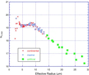
ratio and τ is the cloud optical depth. From Mie calcula-tions based on in situ measurements of water cloud size dis-tributions (Hu et al., 2006; also see Fig. 2), SWC is found

to vary insignificantly for a wide variety of water clouds, having a mean value of 18.9 sr and a standard deviation of 0.25 sr over ocean and 0.47 sr over land. The presence of a semi-transparent aerosol layer above an OWC will reduce

γ_{WC, SS, NA}′ (r)by an amount equal to the two-way transmit-tance, exp(−2τaerosol), of the aerosol layer; i.e., γ_{WC, SS}′ =

16 17 18 19 20 21

0 5 10 15 20 25 30

continental

marine

artificial SC,53

2

Effective Radius (m)

Figure 2.Water cloud lidar ratios calculated as function of effective

droplet radius; red crosses and blue diamonds use in situ measure-ments of droplet radius (Miles et al., 2000), whereas green squares are derived from modeled distributions for clouds having larger droplet sizes.

of the overlying aerosol layer (Hu et al., 2007). Therefore,

τaerosol= −

1 2ln

γ_{WC, SS}′

γ_{WC, SS, NA}′ !

. (6a)

τ_aerosol= −1

2ln

H γ_{WC, TS}′ 1 2SWC

!

(6b)

= −1

2ln 2SWCγ ′

WC, TS

_1−δ

I

1+δI

2!

.

The layer-integrated depolarization ratio within the cloud layer, δI, is calculated from the perpendicular and parallel

components of attenuated backscatter measured at 532 nm,

β′

⊥andβ||′,

δI= RrWC, top

rWC, baseβ

′ ⊥(r)dr

RrWC, top

rWC, baseβ

′ ||(r)dr

. (7)

The AOD determined using the OWC technique can be used as a constraint to retrieve the backscatter and extinction pro-files and lidar ratio of the overlying aerosol layer. For the cases selected and analyzed in this paper, the underlying clouds are opaque boundary layer clouds with cloud-tops lower than 2 km. Given the relatively small footprint of the CALIOP lidar (100 m), for single-shot retrievals, it is not necessary that the clouds be overcast on any significant hori-zontal scale, and the retrieval appears to work even in broken stratocumulus. A closer examination shows that the temper-atures at the top of these opaque clouds typically range from 8◦_{to 25}◦_{, confirming that these clouds are water.}

Retrievals from measurements made by passive satellite sensors such as MODIS (Zhang and Platnick, 2011) produce effective radii for water clouds that are often larger than those

obtained from in situ measurements (Miles et al., 2000). To represent these larger droplet sizes we have extended the previously reported Mie calculations to cloud particle sizes larger than 15 µm. The results are presented in Fig. 2 (solid green squares). For these larger effective radii, the water cloud lidar ratio shows a significant dependence on droplet size. Furthermore, the possibility of encountering these large droplet sizes precludes the use of a theoretical calculation of

SWC and highlights the need to use an empirically derived,

location-dependentγ_{WC, SS, NA}′ in the OWC AOD retrieval. We examined γ_{WC, SS, NA}′ and SWC=1/2γWC,SS,NA′ for

opaque water clouds based on the CALIOP measure-ments made during June–September from years 2007–2012.

γ_{WC, SS, NA}′ is calculated usingγ_{WC, SS, NA}′ =γ_{WC, TS, NA}′ H, whereγ_{WC, TS, NA}′ =RrWC,base

rWC,top B

′_{(r)dris the integrated} atten-uated backscatter of an opaque water cloud layer,rbase and rtopare, respectively, the base and top of the cloud and H is

calculated using Eq. (4) from the layer-integrated depolariza-tion ratioδIof the cloud as defined in Eq. (7). Regional maps

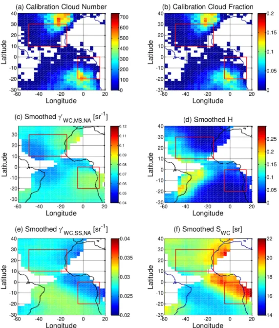
ofγ_{WC, SS, NA}′ andSWCare presented in Fig. 3. Results shown

are based on profiles where no aerosols or clouds were de-tected by the feature finding algorithms above those opaque water clouds with tops below 2 km. To further ensure aerosol-free conditions above the cloud top, the layer-integrated at-tenuated scattering ratio (ASR), R8 km

Ctopβ′dr/

R8 km

Ctopβm′dr−1

was required to lie between−0.05 and 0.05. Figure 3 also shows the spatial dependence of the retrieved values of

γ_{WC, TS, NA}′ (3c), H (3d),γ_{WC, SS, NA}′ (3e) andSWC(3f), with

most OWCs being found over the oceans (panels (3a) and (3b)).SWCis generally larger (i.e., smaller droplet sizes,

re-fer to Fig. 2) over the downwind coastal regions or along the aerosol transport pathways and smaller (larger cloud droplet sizes) in the South Atlantic than in the North Atlantic. This spatial distribution pattern is generally what is expected for the distribution of low cloud droplet sizes. The largest dif-ference between theoretical expectations and the empirically derived values of γ_{WC, SS, NA}′ is a northeastward decreas-ing trend from ∼0.03 to ∼0.023 sr−1 _{seen in the smoke}

transport region. Given this variability, the use of a constant

γ_{WC, SS, NA}′ orSWCcould introduce errors as large as∼0.1 in

the retrieved AOD. For this reason, Eq. (6a) and a regionally varyingγ_{WC, SS, NA}′ are used to derive AOD in this paper. On the other hand,γ_{WC, TS, NA}′ shows a different spatial distribu-tion pattern. It is generally larger over the eastern Atlantic close to the African continent. This may indicate a larger number concentration of the cloud droplets.γ_{WC, TS, NA}′ in-cludes contributions from multiple scattering and multiple scattering generally increases as the number concentration of water droplets increases.

-60 -40 -20 0 20 -30

-20 -10 0 10 20 30 40

L

a

ti

tu

d

e

Longitude

(a) Calibration Cloud Number

0 100 200 300 400 500 600 700

-60 -40 -20 0 20

-30 -20 -10 0 10 20 30 40

L

a

ti

tu

d

e

Longitude

(b) Calibration Cloud Fraction

0 0.05 0.1 0.15 0.2

-60 -40 -20 0 20

-30 -20 -10 0 10 20 30 40

L

a

ti

tu

d

e

Longitude (e) Smoothed 

WC,SS,NA [sr -1_]

0.02 0.025 0.03 0.035 0.04

-60 -40 -20 0 20

-30 -20 -10 0 10 20 30 40

L

a

ti

tu

d

e

Longitude (f) Smoothed S

WC [sr]

14 16 18 20 22

-60 -40 -20 0 20

-30 -20 -10 0 10 20 30

L

a

ti

tu

d

e

Longitude (c) Smoothed 

WC,MS,NA [sr -1_]

0.04 0.05 0.06 0.07 0.08 0.09 0.1 0.11 0.12

-60 -40 -20 0 20

-30 -20 -10 0 10 20 30 40

L

a

ti

tu

d

e

Longitude (d) Smoothed H

0 0.05 0.1 0.15 0.2 0.25

Figure 3. Spatial distributions of(a)number of calibration opaque water clouds above which no other cloud or aerosol layer was

de-tected,(b)the fraction of calibration clouds relative to the total samples in each grid,(c)smoothed mean integrated attenuated backscatter,

γ_{WC, SS, NA}′ =RrWC,top

rWC,baseB′(r)dr, from opaque water clouds in (a), (d) H calculated using Eq. (4),(e)mean integrated attenuated

single-scattering backscatter,γ_{WC, SS, NA}′ = γ_{WC, TS, NA}′ H, calculated from(c)and(d)and used as a reference in each grid box, and(f)water cloud lidar ratioSWC=1/2γ_{WC, SS, NA}′ (i.e., Eq. 5) calculated from(e). The grid box size is 2◦×3◦(lat×long). The smoothing window

is a 10◦_×15◦_{grid. The white color represents the grids having no data samples. Data is from all nighttime CALIOP measurements during} June–August in the years 2007–2012.

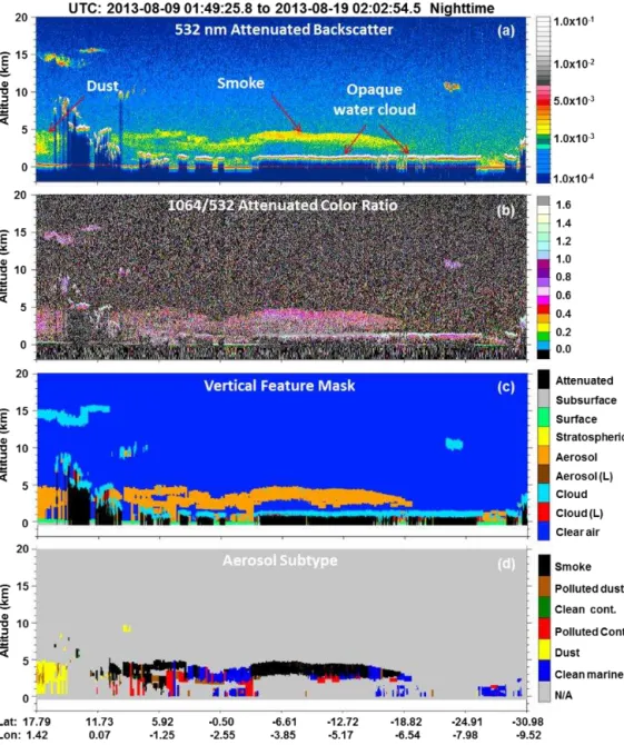
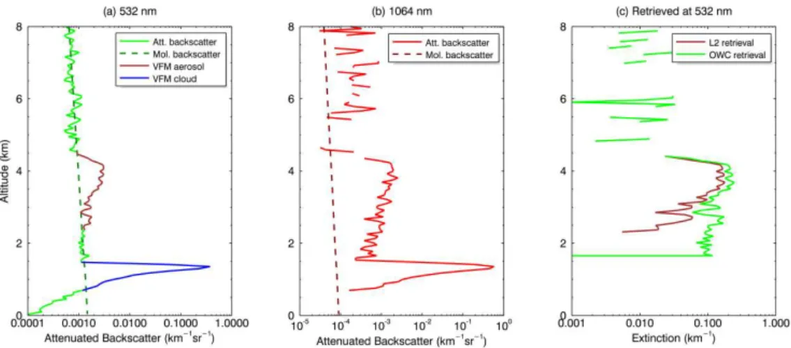
are from a nighttime orbit passing over the western coast of Africa on 19 August 2013. Dust and smoke aerosols and high and low clouds were all observed in this scene. Shown in Fig. 5 are profiles of attenuated backscatter at (a) 532 nm and (b) 1064 nm averaged over 20 km around 10◦_{S in Fig. 2. The} corresponding molecular scattering profiles are indicated by dashed lines. The brown and blue segments in Fig. 5a show a smoke aerosol layer (brown) and an opaque water cloud

Figure 4.Example of CALIOP measurements of aerosols (smoke and dust) over water clouds made on 9 August 2013.(a)532 nm attenuated backscatter,(b)attenuated backscatter color ratio (1064/532),(c)vertical feature mask, and(d)aerosol subtype.

into smoke layers because the extinction of smoke aerosols is typically 2–3 times smaller at 1064 nm than at 532 nm. However, the standard L2 extinction retrieval is only applied in those regions where a layer was detected in the 532 nm profile; i.e., in this example between∼4.5 km and∼2.5 km. Since this same “retrieve in detected layers only” restriction is applied at both wavelengths, and since V3 layer detection is only done at 532 nm, extinction coefficients at 1064 nm are likewise only retrieved between∼4.5 km and∼2.5 km. The averaged 532 nm aerosol extinction profile from the L2 profile products (brown) is shown in Fig. 5c.

The OWC constrained retrieval is initiated at a fixed alti-tude of 8 km and continues downward to an altialti-tude∼0.2 km above the apparent cloud top determined by the L2

mea-Figure 5.Solid curves in panel(a)and(b)show CALIOP attenuated backscatter profiles corrected for attenuation of molecular scattering and ozone absorption 532 nm(a)and 1064 nm(b). The dashed lines in these panels show the corresponding molecular backscatter profiles. Panel(c)shows the aerosol extinction profiles at 532 nm obtained from the standard L2 profile products (brown line) and retrieved in this paper using the OWC constrained technique (light green line). In both cases the retrievals were applied to a sequence of 5 km averaged L1 profiles, which in turn were averaged further for 4 consecutive 5 km profiles around 10◦S, as shown in Fig. 4. Brown and blue coloring in panel(a)indicate the data segments detected as aerosol and cloud in the standard L2 data processing.

sured polarization components of backscattered signals at 532 nm using

δa(r)=

β_⊥′ (r)exp2R8 km

r σa(r)dr

−βm(r)₁₊δm_δm

β_||′(r)exp2R8 km

r σa(r)dr

−βm(r)₁₊1δm

, (8)

whereδ_mis the molecular depolarization ratio, with a value of ∼0.0036 for the spectral bandwidth of the CALIOP re-ceiver (Powell et al., 2009).

In this paper, retrievals using the OWC technique are per-formed on CALIOP V3 L1 attenuated backscatter profiles, averaged horizontally to 5 km. Fifteen recalibrated L1 pro-files are averaged to create each 5 km profile. V3 VFM prod-ucts are used to identify feature locations and find OWCs. The OWCs selected for constrained retrievals are (1) single layered with (2) top heights less than 2 km for which (3) opaque water clouds are detected in all 15 single-shot pro-files within each 5 km average, and the standard deviation of these 15 single shot top heights is less than 50 m. Crite-rion #3 ensures that the cloud tops were relatively uniform throughout the 5 km horizontal extent. The selected OWCs are then sorted into two subsets: those with aerosols located above the clouds and those without (based on the VFM and with|ASR|< 0.05). Imposing a criterion of|ASR|< 0.05 en-sures that the AOD above the clouds is less than∼0.02, even for strongly absorbing aerosols such as smoke. The subset of OWCs with no overlying aerosols in a 2◦_×3◦ _(lat×long) grid box was used to calculate a reference which is used in Eq. (6a) to retrieve AOD from the subset with overlying aerosol. The results shown in Fig. 3 are based on the subset of the opaque water clouds without overlying aerosols.

3.5 Full column retrieval

re--505 -40 -30 -20 10 15 20 25 30 35 L a ti tu d e Longitude (a) Sample Numbers

0 100 200 300 400

-505 -40 -30 -20

10 15 20 25 30 35 L a ti tu d e Longitude (b) AOD, variable _WC

0.2 0.4 0.6 0.8

-505 -40 -30 -20

10 15 20 25 30 35 L a ti tu d e Longitude (c) S_a, variable _WC

30 40 50 60

-505 -40 -30 -20

10 15 20 25 30 35 L a ti tu d e Longitude (d) PDR, variable _WC

0.2 0.25 0.3 0.35 0.4

-505 -40 -30 -20

10 15 20 25 30 35 L a ti tu d e Longitude

(e) Number of Samples, ASR>0.3

0 100 200 300 400

-505 -40 -30 -20

10 15 20 25 30 35 L a ti tu d e Longitude (f) AOD, variable _WC, ASR>0.3

0.2 0.4 0.6 0.8

-505 -40 -30 -20

10 15 20 25 30 35 L a ti tu d e Longitude (g) S_a, variable _WC, ASR>0.3

30 40 50 60

-505 -40 -30 -20

10 15 20 25 30 35 L a ti tu d e Longitude

(h) PDR, variable _WC, ASR>0.3

0.2 0.25 0.3 0.35 0.4

-505 -40 -30 -20

10 15 20 25 30 35 L a ti tu d e Longitude (i) Fraction 0 0.1 0.2

-505 -40 -30 -20

10 15 20 25 30 35 L a ti tu d e Longitude (j) AOD, constant _WC, ASR>0.3

0.2 0.4 0.6 0.8

-505 -40 -30 -20

10 15 20 25 30 35 L a ti tu d e Longitude (k) S_a, constant _WC, ASR>0.3

30 40 50 60

-505 -40 -30 -20

10 15 20 25 30 35 L a ti tu d e Longitude

(l) PDR, constant _WC, ASR>0.3

0.2 0.25 0.3 0.35 0.4

-505 -40 -30 -20

10 15 20 25 30 35 L a ti tu d e Longitude (m) Fraction, ASR>0.3

0 0.1 0.2

-505 -40 -30 -20

10 15 20 25 30 35 L a ti tu d e Longitude (n) AOD, ASR>0.3

-0.2 -0.1 0 0.1 0.2 0.3

-505 -40 -30 -20

10 15 20 25 30 35 L a ti tu d e Longitude (o) S_a, ASR>0.3

-20 -10 0 10 20

-505 -40 -30 -20

10 15 20 25 30 35 L a ti tu d e Longitude (p) PDR, ASR>0.3

-0.05 0 0.05

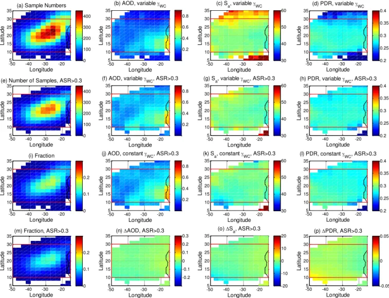
Figure 6.Analysis results in the dust region over the eastern North Atlantic from CALIOP data acquired during June–August in the years

2007–2012.(a)Number of samples,(b)AOD retrieved using the OWC technique with a location-dependentγ_WCfor aerosol layers located above the opaque water clouds, and(c)Saand(d)particulate depolarization ratio (PDR) retrieved using the OWC-retrieved AOD in(b)as a constraint. Shown in the second row of panels(e–h)are corresponding maps with data screening of ASR > 0.3 for the overlying aerosol layers (i.e., relatively weakly scattering aerosol layers are excluded). Panels (i)and(m)show the fraction of OWC retrievals relative to the total number of measurements in each grid, respectively, for all aerosol layers and moderately dense aerosol layers. The third row of panels(j–l)are corresponding maps using a constantγ_{WC, SS, NA}′ (0.0270 sr−1)averaged over the spatial domain indicated by the red box. The bottom row of panels(n–p)are the difference of the corresponding quantities retrieved using a constantγ_{WC, SS, NA}′ and a location-dependentγ_{WC, SS, NA}′ . The size of each grid box is 2◦_×3◦_{(lat×long). The spatial variability in the intrinsic dust optical propertiesS}

aand

PDR is seen to be larger for the retrievals that use a constantγ_WC,SS,NA′ (kandl) than for those that use a location-dependentγ_{WC, SS, NA}′

(gandh).

trieval is only applied to the upper part of this layer between

∼5 km and∼3 km and hence misses the lower part of the layer between ∼3 km and ∼1.5 km and underestimate the AOD of the layer (e.g., see Kim et al., 2013, Torres et al., 2013). Because the FC algorithm performs the retrieval from 8 km down to the cloud top at∼1.5 km, the optical depths re-trieved by the FC method provide a useful reference to diag-nose and evaluate failures to detect the full extent of aerosol layers in the standard retrieval.

4 Results

Re--5 0 5 10 15 -20 -15 -10 -5 0 L a ti tu d e Longitude (a) Sample Numbers

0 200 400 600 800 1000 1200

-5 0 5 10 15

-20 -15 -10 -5 0 L a ti tu d e Longitude (b) AOD, variable _WC

0 0.2 0.4 0.6 0.8

-5 0 5 10 15

-20 -15 -10 -5 0 L a ti tu d e Longitude (c) S_a, variable _WC

50 60 70 80 90

-5 0 5 10 15

-20 -15 -10 -5 0 L a ti tu d e Longitude (d) PDR, variable _WC

-0.1 -0.05 0 0.05 0.1 0.15

-5 0 5 10 15

-20 -15 -10 -5 0 L a ti tu d e Longitude

(e) Number of Samples, ASR>0.2

0 200 400 600 800 1000 1200

-5 0 5 10 15

-20 -15 -10 -5 0 L a ti tu d e Longitude (f) AOD, variable _WC, ASR>0.2

0 0.2 0.4 0.6 0.8

-5 0 5 10 15

-20 -15 -10 -5 0 L a ti tu d e Longitude (g) S_a, variable _WC, ASR>0.2

50 60 70 80 90

-5 0 5 10 15

-20 -15 -10 -5 0 L a ti tu d e Longitude (h) PDR, variable _WC, ASR>0.2

-0.1 -0.05 0 0.05 0.1 0.15

-5 0 5 10 15

-20 -15 -10 -5 0 L a ti tu d e Longitude (i) Fraction 0 0.1 0.2 0.3 0.4 0.5

-5 0 5 10 15

-20 -15 -10 -5 0 L a ti tu d e Longitude

(j) AOD, constant _WC, ASR>0.2

0 0.2 0.4 0.6 0.8

-5 0 5 10 15

-20 -15 -10 -5 0 L a ti tu d e Longitude (k) S_a, constant _WC, ASR>0.2

50 60 70 80 90

-5 0 5 10 15

-20 -15 -10 -5 0 L a ti tu d e Longitude (l) PDR, constant _WC, ASR>0.2

-0.1 -0.05 0 0.05 0.1 0.15

-5 0 5 10 15

-20 -15 -10 -5 0 L a ti tu d e Longitude (m) Fraction, ASR>0.2

0 0.1 0.2 0.3 0.4 0.5

-5 0 5 10 15

-20 -15 -10 -5 0 L a ti tu d e Longitude (n) AOD, ASR>0.2

-0.2 -0.1 0 0.1 0.2 0.3

-5 0 5 10 15

-20 -15 -10 -5 0 L a ti tu d e Longitude (o) S_a, ASR>0.2

-20 -10 0 10 20

-5 0 5 10 15

-20 -15 -10 -5 0 L a ti tu d e Longitude (p) PDR, ASR>0.2

-0.05 0 0.05

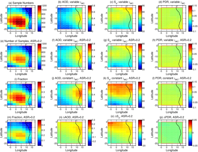
Figure 7.Analysis results in the smoke region over the eastern South Atlantic from CALIOP data acquired during the months of July–

September in the years 2007–2012.(a)Number of samples,(b)AOD retrieved using the OWC technique with a location-dependentγW C for aerosol layers located above the opaque water clouds, and(c)Saand(d)particulate depolarization ratio (PDR) retrieved using the OWC-retrieved AOD in(b)as a constraint. Shown in the second row of panels(e–h)are corresponding maps with data screening of ASR > 0.2 for the overlying aerosol layers (i.e., relatively weakly scattering aerosol layers are excluded). Panels(i)and(m)show the fraction of OWC retrievals relative to the total number of measurements in each grid, respectively, for all aerosol layers and moderately dense aerosol layers. The third row of panels(j–l)are corresponding maps using a constantγ_{WC, SS, NA}′ (0.0260 sr−1)averaged over the spatial domain indicated by the red box. The bottom row of panels(n–p)show the difference of the corresponding quantities retrieved using a constantγ_{WC, SS, NA}′

and a location-dependentγ_{WC, SS, NA}′ . The size of each grid box is 2◦_×3◦_{(lat×long). A significant location-dependent trend is seen in the} smokeSa(j)retrieved using a constantγ_{WC, SS, NA}′ .

sults are presented and discussed in the following subsec-tions.

4.1 Spatial distributions from OWC retrievals

Because accurate knowledge ofγ_{WC, SS, NA}′ is very important in the derivation of AOD using the OWC technique, in this subsection we examine the spatial variability ofγ_{WC, SS, NA}′

and its potential impact on the retrieved AODs. To obtain more insight we look into the spatial distributions of dust

and smoke optical properties retrieved using the OWC tech-nique. Figures 6 and 7 present 2◦_×3◦ _{resolution maps of} (a) the number of samples acquired, (b) mean AODOWC,

(c) meanSaand (d) PDR of aerosol layers using the OWC

constrained retrieval technique, respectively, for the dust and smoke transport regions. AODOWC was calculated

0 10 20 30 40 50 60 70 80 90 0

0.2 0.4 0.6 0.8 1 1.2 1.4

Sa (sr)

A

O

DO

W

C

(a)

0 20 40 60 80 100 120

0 0.1 0.2 0.3 0.4 0.5 0.6 0

20 40 60 80 100

PDR

Sa

(

sr

)

(b)

0 20 40 60 80 100 120

0 10 20 30 40 50 60 70 80 90 0

20 40 60 80 100 120

Sa (sr)

O

ccu

rr

e

n

ce

N

u

m

b

e

r

(c)

50.5 /45.5 /44.0 26.4

45.1 /44.4 /43.3 8.8, ASR>0.3

0 0.1 0.2 0.3 0.4 0.5 0.6 0

50 100 150 200

PDR

O

ccu

rr

e

n

ce

N

u

m

b

e

r

(d) 0.222 /0.277 /0.280 4.24 0.281 /0.281 /0.283 0.044, ASR>0.3

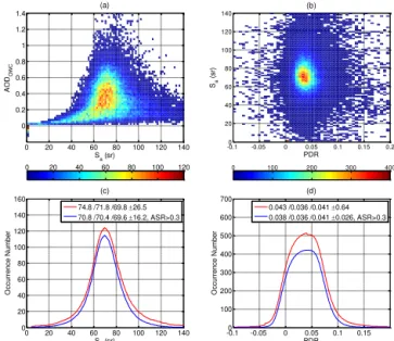
Figure 8.Analysis results for the dust transport region as indicated

by the red box in Fig. 6. The upper row shows two-dimensional (2-D) distributions of(a)OWC AOD vs.Saretrieved using OWC

AOD as a constraint,(b)Savs. PDR, while the lower row shows

histograms of(c)Saand(d)PDR occurrence frequencies. TheSa

distribution in(c)has a bin size of 0.1 sr and is smoothed, while the bin size forSain(a)and(b)is 1.5 sr. The PDR distribution in (c)has a bin size of 0.001 and is smoothed, while the bin size in

(b)is 0.006. The red curves in(c)and(d)include all data and the blue curves are screened data using ASR > 0.3. The numbers in the legends of are mean/median/mode±standard deviation of Sa (c)

and PDR(d).

smoke region is smaller than for the dust region because for the same extinction the backscatter at 532 nm is smaller for smoke than dust due to the difference in the lidar ratios. Pan-els (j) through (l) in each figure are the corresponding prop-erties retrieved using a constant value of γ_{WC, SS, NA}′ which was averaged over the entire red box for each selected spatial domain, and panels (n) through (p) are the differences be-tween these retrieved properties using a location dependent

γ_{WC, SS, NA}′ (as in panels (j)–(l)) and a constantγ_{WC, SS, NA}′

(as in panels (f)–(h)).

Most OWCs are observed just offshore over the northeast-ern and southeastnortheast-ern Atlantic, in the trade wind regions. As expected, AODOWCis the largest in the coastal regions near

the sources in northern and southern Africa and decreases gradually as dust or smoke is transported farther from the sources.

The Sa retrieval is sensitive to errors and biases in the

AODOWCand to the noise in the above-cloud backscatter

sig-nals. This is especially noticeable when the overlying aerosol layers are optically thin, as will be discussed further in the following subsections. Partly due to this, we see large vari-ations in the retrieved Sa at the edges of the dust transport

pathway (Fig. 6c) where AODOWCis small (Fig. 6b). We also

see that the retrievedS_avalues are larger outside of the typ-ical dust transport pathway, where the occurrence of dust is less frequent. The PDR, retrieved using Eq. (8) and shown in Fig. 6d, generally has smaller values north of ∼30◦N and south of ∼10◦_{N, which suggests that relatively large} amounts of other aerosol types are present outside of the dust transport pathway. North of∼30◦_{N the westerly wind} (Fig. 1) can carry anthropogenic aerosols having largeSa

val-ues from North America to the northwest coast of Africa. South of ∼10◦_{N, the southeasterly trade wind can bring} biomass burning aerosol from central Africa to the tropical North Atlantic (Fig. 1). At 532 nm, biomass burning aerosols (smoke) generally haveSavalues larger than dust, as seen by

comparing Fig. 7c and g to Fig. 6c and g. The retrievedSaand

PDR for dust are distributed more uniformly when weakly scattering aerosol layers are screened out using ASR > 0.3. This is as generally expected and instills confidence in our analysis results. Since a sizeable fraction of North Africa is covered by deserts, desert dust is a dominant aerosol type in this region all year long. During summer, the transport of dust over the Atlantic is usually confined to the free tropo-sphere by two inversions and hence the dust size distribution can remain largely unchanged during the course of transport across the Atlantic Ocean (Maring et al, 2003). More uni-form distributions of meanSa and PDR are expected where

dust is dominant. Large values (> 60 sr) are, however, still seen south of 10◦_{N, where the transported biomass burning} aerosol is relatively dense and dominant. We note that while the meanSa shown in Fig. 6 has a relatively uniform

spa-tial distribution, the individual values ofSaaveraged in each

grid box vary considerably. As will be discussed in the next subsection (see Fig. 8), this variability inS_a may reflect an underlying variability in the origin of different dust plumes. The relatively uniform distribution of the meanSamay

sim-ply indicate that, within each grid box, the probabilities of dust transport originating from different source regions are similar.

When a constantγ_{WC, SS, NA}′ (or SWC)is used, as in the

previous work of Chand et al. (2009) and Sakaeda et al. (2011), a larger spatial trend is seen both in theSa(Fig. 6k)

and the PDR (Fig. 6l) retrieved for dust. A more significant trend is also seen in the retrievedSafor smoke (Fig. 7k). The

large spatial trend in the retrievedSaespecially in the smoke

transport region when using a constantγ_{WC, SS, NA}′ does not appear to be realistic and is correlated with theγ_{WC, SS, NA}′

distribution in Fig. 3, indicating that the large trend in the aerosol retrievals is actually an artifact introduced by the use of a constantγ_{WC, SS, NA}′ . The use of a constantγ_{WC, SS, NA}′

can overestimate smoke AOD by∼0.1 near the source and

Saby∼10 sr in the northern part of the selected smoke

0 10 20 30 40 50 60 70 80 90 0

0.05 0.1 0.15 0.2 0.25 0.3 0.35 0.4 0.45 0.5

S

a (sr)

P

D

R

(a) CALIOP OWC Retrieval

0 20 40 60 80 100 120

0 10 20 30 40 50 60 70 80 90 0

0.05 0.1 0.15 0.2 0.25 0.3 0.35 0.4 0.45 0.5

S

a (sr)

P

D

R

(b) HSRL Caribbean 2010

0 0.5 1 1.5 2 2.5 x 104

Marine + dust

Urban/Smoke Dust

Marine

Smoke Dust

Figure 9.2-D distributions of lidar ratio and PDR(a)retrieved

us-ing the OWC constrained technique from six years of the CALIOP measurements and (b) measured by the NASA LaRC airborne HSRL during nine CALIOP validation flights during 11–28 Au-gust 2010 over the Caribbean Sea (see Burton et al., 2012 for more details about this validation campaign). Panel (a)is a composite plot made from the OWC constrained retrievals from the dust trans-port region (i.e., Fig. 8b) and from the smoke transtrans-port region (i.e., Fig. 10b, with the sample number being scaled by a factor of 1/3). Note that each CALIOP sample was obtained for a layer extending from cloud top to 8 km, whereas each HSRL sample was measured for a 300 m range bin.

4.2 Dust intrinsic optical properties

One-dimensional (1-D) and two-dimensional (2-D) his-tograms of the retrieved Sa and PDR using a

location-dependent γ_{WC, SS, NA}′ within the spatial domain as defined by the red box over the dust transport region are presented in Fig. 8a–d. The distributions of the retrievedS_aand PDR (Fig. 8c, d) are somewhat asymmetric. The mean value of the dust lidar ratio distribution is 50.5 sr, with a median of 45.5 sr, a mode of 44.0 sr, and a standard deviation of 26.4 sr, while for the PDR distribution the mean is 0.222, the me-dian is 0.277, the mode is 0.280, and the standard deviation is 4.24 (this large value is due to a few outliers that have huge values). When weakly scattering layers are screened out us-ing ASR > 0.3, the Sa and PDR distributions become more

0 20 40 60 80 100 120 140 0

0.2 0.4 0.6 0.8 1 1.2 1.4

S_a (sr)

A

O

DO

W

C

(a)

0 20 40 60 80 100 120

-0.10 -0.05 0 0.05 0.1 0.15 0.2

20 40 60 80 100 120 140

PDR

Sa

(

sr

)

(b)

0 100 200 300 400

0 20 40 60 80 100 120 140 0

20 40 60 80 100 120 140 160

S_a (sr)

O

ccu

rr

e

n

ce

N

u

m

b

e

r

(c) 74.8 /71.8 /69.8 26.5 70.8 /70.4 /69.6 16.2, ASR>0.3

-0.10 -0.05 0 0.05 0.1 0.15 100

200 300 400 500 600 700

PDR

O

ccu

rr

e

n

ce

N

u

m

b

e

r

(d) 0.043 /0.036 /0.041 0.64 0.038 /0.036 /0.041 0.026, ASR>0.3

Figure 10.Analysis results for the smoke transport region as

indi-cated by the red box in Fig. 7. The upper row shows 2-D distribu-tions of(a)AODOWC vs.Sa retrieved using AODOWC as a

con-straint and(b)Savs. PDR, while the lower row shows histograms

of(c)Saand(d)PDR occurrence frequencies. TheSadistribution

in(c)has a bin size of 0.1 sr and is smoothed, while the bin size for

Sain(a)and(b)is 1.5 sr. The PDR distribution in(d)has a bin size

of 0.001 and is smoothed, while the bin size in(b)is 0.006. The bin size for AOD in(b)is 0.025. The red curves in(c)and(d)include all data and the blue curves are screened data using ASR > 0.2. The numbers in the legends of are mean/median/mode±standard devi-ation ofSa(c)and PDR(d).

symmetric. The mean, median, mode and standard deviation of the screenedSadata are, respectively, 45.1, 44.4, 43.3 and

8.8 sr, and, respectively, 0.281, 0.281, 0.283 and 0.044 for the screened PDR data. For either the screened or the un-screened data, the modeledSavalue (40 sr) used to produce

CALIOP V3 data is∼10 % smaller than the OWC retrieved value (Fig. 8c).

The dustSavalues reported in this work fall well within

the range of the natural variability of dust lidar ratios pre-viously reported in the scientific literature. An earlier case study based on CALIOP measurements (Liu et al., 2008) tracked a dust event that occurred on 17 August 2006 in North Africa and was subsequently transported across the Atlantic Ocean over the course of several days. The retrieved

distribution for opaque dust layers (AOD>∼2) over North Africa with a mean value of 38.5±9.2 sr. It was shown that multiple scattering in these opaque dust layers can decrease the effective lidar ratio by 10 % or more relative to the semi-transparent layers analyzed here with the OWC technique.

Shipborne Raman lidar measurements in May 2013 tracked the Saharan air layer across the tropical Atlantic (Kanitz et al., 2014). A 532 nmSaof 45 sr was measured for

aged dust that was∼4500 km away from the North Africa, and 50 sr for dust∼800 km off the coast of the North Africa. The layers observed ∼800 km off the coast were not pure dust, but instead were dust mixed with smoke which gen-erally has higher Sa values than dust. Over dust source

re-gions in Morocco, Sa was observed in a range of 38–50 sr

by an airborne HSRL for pure dust over Morocco during the SAMUM 2006 campaign (Esselborn et al., 2009). Mean-while, a range of 53–55±7 sr was observed for selected dust events by ground-based Raman lidars operated at the airport of Ouarzazate in Morocco (Tesche et al., 2009). Back trajec-tory analyses show that the observed variability in lidar ra-tio is primarily attributable to differences in source regions. The large deviation of Saretrieved in this study (Fig. 8a, c)

may partly reflect the dependence of the dust optical proper-ties on the sources. Computations based on in situ measure-ments (Omar et al., 2010) and AERONET retrievals (Cattrall et al., 2005; Schuster et al., 2012) also produce dustSavalues

that vary from∼40 sr to∼55 sr depending on the observa-tion sites. In the remote transport sites in the Gulf of Mex-ico and the Caribbean Sea,Savalues measured by the LaRC

HSRL for an apparently pure dust (depolarization ratio of 0.31–0.33) transported from the North Africa range from 45 to 51 sr (Burton et al., 2013).

PDR is another intrinsic optical property of aerosols. Dust generally has relatively large PDRs due to the irregular shapes and large sizes of dust particles compared with other types of aerosol. Pure dust can have a PDR larger than 0.3. As with the lidar ratios, the dust PDRs reported in this work are consistent with previously reported values. The PDR ob-tained in the CALIOP case study mentioned earlier (Liu et al., 2008) is∼0.32, and this remained nearly unchanged dur-ing the course of the dust transport from the source into the Gulf of Mexico. For a four month data set of CALIPSO mea-surements, the PDR retrieved for all single dust layers with optical depths greater than 0.1 over the North Africa has a mean value of 0.3±0.07 (Liu et al., 2011). The PDR value measured at 532 nm for pure dust layers during the SAMUM 2006 campaign is 0.31±0.03 (Freudenthaler et al., 2009; Es-selborn et al., 2009). In the Caribbean Sea, the transported pure Sahara dust has PDRs ranging from 0.30 to 0.35 (Bur-ton et al., 2013). The retrieved PDR for the relatively dense aerosol layers (ASR > 0.3) over the North Atlantic reported in this paper has a median value of 0.281±0.044, indicating that these aerosol layers are dominated by dust particles. For the weakly scattering layers (refer to Fig. 6), the retrieved

Sa tends to be larger and PDR tends to be smaller,

imply-ing that the relative concentration of dust particles is smaller compared with the optically thick cases. These optically thin layers are most likely mixtures of dust and continental pollu-tion or biomass burning smoke.

For comparison we present in Fig. 9b the measurements made by the LaRC HSRL during nine CALIOP validation flights during 11–28 August 2010 over the Caribbean Sea. Based on the classification scheme by Burton et al. (2012), four major modes are seen – dust (North Africa origin), ma-rine, a mixture of dust and mama-rine, and urban/smoke. In ad-dition, there is a transitional leg between the urban/smoke mode and the marine+dust mode which can be a mixture of these two types of aerosol. Shown in Fig. 9a is a compos-ite distribution made from the OWC constrained retrieval for the spatial domain along the Saharan dust transport pathway over the North Atlantic (i.e., Fig. 8b) and for the spatial do-main along the smoke transport pathway over the South At-lantic (i.e., Fig. 10b). The OWC retrieved distribution is seen to compare very well with the HSRL measured distribution for dust, although the PDR measured by CALIOP is noisier than that by HSRL. The mode values for the dustSaand PDR

measured by HSRL are∼44.5 sr and∼0.315, respectively. 4.3 Smoke intrinsic optical properties

Figure 10 shows results from the spatial domain indi-cated by the red box in Fig. 7. The Sa values retrieved

using AODOWC as a constraint have mean/median/mode

values of 74.8/71.8/69.8±26.5 sr for all the data and 70.8/70.4/69.6±16.2 sr for screened data. TheSa

distribu-tion in the smoke region (Fig. 7g) is not as uniform as in the dust region (Fig. 6g) even after screening out weakly scattering layers. Unlike North Africa, where the landmass is largely desert and desert dust is a dominant aerosol type, in central and southern Africa, the human population den-sity is higher and the surface type is more variable. While smoke is the dominant aerosol type during the austral win-ter, when biomass burning is active, several other types of anthropogenic aerosols can also be present in non-negligible amounts during this time period.

Smoke from biomass fires is dominated by submicron-sized particles, frequently containing internally mixed black carbon (Reid et al., 2005, Li et al., 2003), and produces low PDR and highSaat 532 nm (Müller et al., 2007; Omar et al.,

2009; Burton et al., 2013). SmokeSaand PDRs can vary

de-pending on the type of fire, the combustion source and the age of the smoke. TheS_a values retrieved in this study are consistent with the case study presented in Hu et al. (2007) that used the OWC constrained technique and obtained anSa

-0.2 0 0.2 0.4 0.6 0.8 1 1.2 1.4 0 0.2 0.4 0.6 0.8 1 1.2 1.4 AOD OWC A O DL2 (a)

-0.2 0 0.2 0.4 0.6 0.8 1 1.2 1.4

0 0.2 0.4 0.6 0.8 1 1.2 1.4 AOD OWC A O DL 2 ,r e sca le d (b)

-0.2 0 0.2 0.4 0.6 0.8 1 1.2 1.4

0 0.2 0.4 0.6 0.8 1 1.2 1.4 AOD OWC A O DF C ,m o d e l ( Sa = 4 0 ) (c) 0 50 100 150 200 250 300 350 400 450 500

10-4 10-3 10-2 10-1

0 1 2 3 4 5 6 7 8 A lt it u d e ( km )

Extinction (km-1₎

(d)

L2 L2 Rescaled OWC FC S

a= 40 FC S

a= 45

-0.20 0 0.2 0.4 0.6 0.8 1 1.2

500 1000 1500 2000 2500 3000

L2 Subtype AOD

O ccu rr e n ce N u m b e r (e) Marine (0.02%) Dust (91.35%) Poll. dust (8.52%) Poll. Cont. (0.02%) Clean Cont. (0.06%) Smoke (0.19%)

-0.20 0 0.2 0.4 0.6 0.8 1 1.2

500 1000 1500 2000 2500 3000 3500 4000 AOD O ccu rr e n ce N u m b e r (f) L2 (AOD=0.183) L2 Rescaled (0.177) OWC (0.247) FC S

a=40 (0.202) FC S_a=45 (0.258)

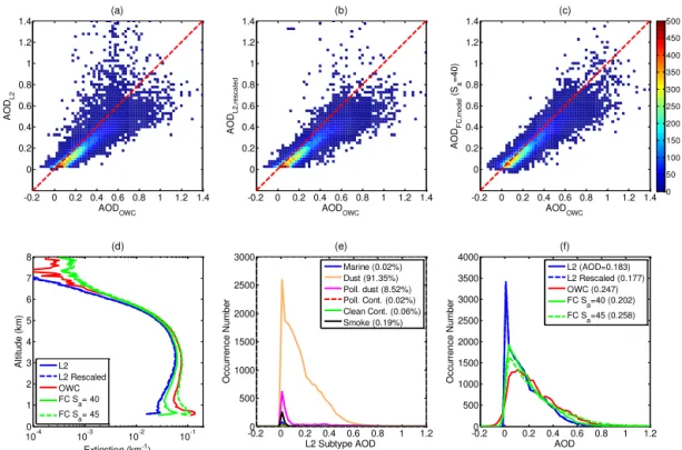
Figure 11.Analysis results for the dust transport region as indicated by the red box in Fig. 6. The top row shows 2-D distributions of

(a)AODL2vs. AODOWC,(b)AODL2,resvs. AODOWC, and(c)AODFC, modvs. AODOWCforSa= 40 sr. The bottom row shows(d)mean

extinction profiles and histograms of occurrence number, (e)L2 AOD of different aerosol types, and(f)AOD retrieved using different retrieval methods. The bin size for AOD is 0.025.

column AOD was dominated by smoke, values of 70–74 sr were obtained by combining airborne backscatter lidar data with ground-based sun photometer data (McGill et al., 2003). The PDR values retrieved in the smoke region are typ-ically smaller than 0.1, with mean/median/mode values of 0.043/0.036/0.041±0.64 for all smoke layers analyzed and 0.038/0.036/0.041±0.026 for the layers with ASR > 0.2. Ir-respective of aerosol type, the PDR calculation can be bi-ased significantly by noise when the aerosol layer is weakly scattering. The standard deviation computed from all the an-alyzed smoke layers is large (0.64), but is reduced to 0.026 when weakly scattering layers are screened out. The PDR distributions appear to be non-Gaussian with a positive skew-ness. Internally mixed potassium salts and organic parti-cles are the predominant components in the smoke from the African biomass burning, and the smoke particles undergo hygroscopic growth, reaction and transformation (Reid et al., 2005). Although dominated by fine mode particles, large complex chain-like soot aggregates and aggregates of fine particles have been observed in the smoke from the biomass burning in the southern Africa (Li et al., 2003). Unlike the surrounding fine mode particles, these large nonspherical particles can strongly depolarize the incident photons and the depolarization ratio of measured backscatter signals from smoke varies depending on the fraction of nonspherical

par-ticles (Martins et al., 1998; Murayama et al., 2004; Sun et al., 2013).

The OWC smoke retrieval compares well with the urban/smoke category measured by HSRL during the Caribbean 2010 campaign shown in Fig. 9b. Although the distribution for the urban/smoke category is complex because of the mixing with marine and dust, the mode values forSa

and PDR are∼69.5 sr and∼0.025, respectively, consistent with the OWC retrieved mode values.

4.4 CALIOP L2 AOD evaluation

In this subsection, we attempt to evaluate above-cloud AOD produced by the CALIOP L2 standard retrieval and estimate an error budget based on the analysis of the two selected re-gions. Figures 11 and 12 present comparisons of the analysis results where the OWC retrieval is considered to be “truth”. For the dust transport region, as shown in Fig. 11a, the ma-jority of AODL2-AODOWCscatter falls on a line with a slope

of∼0.75 (the fit curve is not shown). The mean value for AODL2 is 0.183 (Fig. 11f), which is 25.9 % smaller than

the mean value of AODOWC (0.247). We examine the

oc--0.2 0 0.2 0.4 0.6 0.8 1 1.2 1.4 0 0.2 0.4 0.6 0.8 1 1.2 1.4 AOD_OWC A O DL2 (a)

-0.2 0 0.2 0.4 0.6 0.8 1 1.2 1.4

0 0.2 0.4 0.6 0.8 1 1.2 1.4 AOD_OWC A O DL 2 ,r e sca le d (b)

-0.2 0 0.2 0.4 0.6 0.8 1 1.2 1.4

0 0.2 0.4 0.6 0.8 1 1.2 1.4 AOD_OWC A O DF C ,m o d e l ( Sa = 7 0 ) (c) 0 100 200 300 400 500 600

10-4 10-3 10-2 10-1 100

0 1 2 3 4 5 6 7 8 A lt it u d e ( km )

Extinction (km-1₎

(d) L2 L2 Rescaled OWC FC S a=70 FC S a=75

-0.20 0 0.2 0.4 0.6 0.8 1 1.2

1000 2000 3000 4000 5000 6000 7000 8000 9000

L2 Subtype AOD

O ccu rr e n ce N u m b e r (e) Marine (4.46%) Dust (0.24%) Poll. dust (8.35%) Poll. Cont. (3.89%) Clean Cont. (0.01%) Smoke (83.34%)

-0.20 0 0.2 0.4 0.6 0.8 1 1.2

1000 2000 3000 4000 5000 6000 7000 8000 9000 AOD O ccu rr e n ce N u m b e r (f)

L2 (AOD= (0.191) L2 Rescaled (0.222) OWC (0.311) FC S

a=70 (0.314) FC S

a=75 (0.384)

Figure 12.Analysis results for the smoke transport region as indicated by the red box in Fig. 7. The top row shows 2-D distributions of(a)

AOD_L2vs. AOD_OWC,(b)AOD_{L2, res}vs. AOD_OWC, and(c)AOD_{FC, mod}vs. AOD_OWC forSa= 70 sr. Full column AOD using modeled

dustSa=40 sr vs. AODOWC. The bottom row shows(d)extinction profiles and histograms of occurrence number,(e)L2 AOD of different

aerosol types, and(f)AOD retrieved using different retrieval methods. The bin size for AOD is 0.025.

cur in the dust region (∼2.5 % of the retrievals), and are hereafter excluded to simplify the remaining analysis. The CALIOP aerosol classification (Fig. 11e) is dominated by “dust” (contributing 91.4 % of the total AOD), followed by “polluted dust” (8.5 %), consistent with expectations for the area. Assuming that any aerosol type in this region other than “dust” is a misclassification, rescaling the extinction of all non-“dust” range bins using Eq. (3) decreases the AOD by only 0.006. This accounts for only 9.4 % of the AOD dis-crepancy. This small change indicates that the CALIOP L2 algorithms have been largely successful in correctly identi-fying the above-cloud aerosol type as “dust” in this region.

As mentioned earlier, the FC retrieval using a fixed Sa

can provide insight into the error due to the failure of the L2 algorithms to detect the full vertical extent of aerosol layers. The mean AOD from the FC retrieval using the modeled Sa,model value (40 sr) for “dust” (AODFC,model)

is 0.202, which is larger than that for the rescaled L2 AOD (AODL2,rescaled= 0.177) by 0.025, but still smaller than

AODOWC by 0.045. We note that AODL2,rescaled was

de-rived by scaling all other aerosol types to “dust” using Eq. (3). Therefore, the difference between AODFC,modeland

AODL2,rescaledis mainly due to the failure to detect the full

extent of the aerosol layers (e.g., due to inherent detection limits). The failure to detect those parts of the aerosol layer(s) that lie below the CALIOP detection limit may contribute

under half (39.1 %; see Tables 1 and 2) of the total AOD dis-crepancy. From Fig. 11d we can see that the difference be-tween AODL2,rescaled and AODFC,model comes mainly from

the extinction retrieval at lower altitudes. Below 1 km there may be some contamination by cloud edges. Although the L2 algorithms fail to detect the aerosol above about 7 km (Fig. 11d), the aerosol loading here is very small and does not contribute significantly to the column AOD. Small dif-ferences between the L2 and FC profiles below 2 km indicate the L2 algorithms are doing a moderately good job of detect-ing the base of the dust layer. The standard CALIOP mod-eledSa,modelfor dust (40 sr) is∼10 % smaller than the OWC

retrieved value (Fig. 8c). Differences inSahave a nonlinear

effect on the retrieved AOD, and thus this 10 % disparity in

Sa contributes the majority (70.3 %) of the total AOD

dis-crepancy. Table 1 compares all AOD retrievals for the dust transport region. Table 2 shows the error budget estimated for AODL2in the dust transport regions along with the error

budget in the smoke transport region that will be discussed in the next paragraph.

In the smoke transport region, the L2 AOD retrieval is not as successful as in the dust transport region. There are two branches in the AODL2-AODOWCdistribution (Fig. 12a). As

seen in Fig. 12f and Table 3, the L2 smoke AOD is 0.191, which is smaller than the smoke AODOWC(0.311) by 38.6 %.

re-0 0.5 1 1.5 0

0.5 1 1.5 2

AOD_OWC

A

O

DFC

(a) FC Retrieval, S_a = 40 (sr)

0 0.5 1 1.5

0 0.5 1 1.5 2

AOD_OWC

A

O

DFC

(b) FC Retrieval, S_a = 45 (sr)

0 0.5 1 1.5

0 0.5 1 1.5 2

AOD_OWC

A

O

DFC

(c) FC Retrieval, S_a = 50 (sr)

0 50 100 150 200 250 300 350

0 0.5 1 1.5

0 0.5 1 1.5 2

AOD_OWC

A

O

DFC

(d) FC Retrieval, S_a = 55 (sr)

0 0.5 1 1.5

0 0.5 1 1.5 2

AOD_OWC

A

O

DFC

(e) FC Retrieval, S_a = 60 (sr)

10-4 10-3 10-2 10-1 100

0 1 2 3 4 5 6 7 8

A

lt

it

u

d

e

(

km

)

Extinction (km-1₎ (f) Extinction Profile

OWC FC40 FC45 FC50 FC55 FC60

Figure 13.Distributions of FC AOD retrieved from the dust transport region using lidar ratios of(a)40,(b)45,(c)50,(d)55 and(e)60 sr

as a function of OWC AOD, and(f)corresponding extinction profiles. The blue line in panel(a–e)has a slope of FCSa/OWCSa. The slope

is(a)40/44.4=0.91,(b)45/44.4=1.01,(c)50/44.4=1.13,(d)55/44.4=1.24, and(e)60/44.4=1.35. The red line is AOD estimated using Eq. (9) for a given lidar ratio used in the FC retrieval.

Table 1.AOD retrievals for dust transport region over North Atlantic.

Different retrievals Mean AOD AOD – AODOWC

(fractional difference)

OWC constrained, AODOWC 0.247

L2 standard, AODL2 0.183 −0.064 (−25.9 %)

L2 rescaled, AODL2, rescaled 0.177 −0.070 (−28.3 %)

Full column (Sa= 40), AODFC, model 0.202 −0.045 (−18.2 %)

Full column (Sa= 45), AODFC,45 0.258 0.011 (4.5 %)

CALIOP subtype Mean L2 AOD L2 AOD fraction

Marine 0.000 0.0 %

Dust 0.168 91.4 %

Polluted dust 0.016 8.5 %

Polluted continental 0.000 0.0 %

Clean continental 0.000 0.1 %

Smoke 0.000 0.2 %

gion, as classified in the CALIOP L2 product, is “smoke” (83.3 % by AOD), which is expected. The next most com-mon type is “polluted dust” (8.4 %), followed by “marine” (4.5 %) and “polluted continental (3.9 %). “Polluted dust” is possible for this area. However, “marine” aerosols are un-likely to be found above the boundary clouds in this region,

dis-Table 2.Error budget estimates∗.

Type Detection Lidar ratio

AODL2−AODL2, res AODOWC−AODL2

AODL2, res−AODFC, model AODOWC−AODL2

AODFC, model−AODOWC AODOWC−AODL2

Dust transport region 9.4 % −39.1 % −70.3 %

Smoke transport region −25.8 % −76.7 % 2.5 %

∗_{Negative values indicate an underestimation and positive values represent an overestimation.}

Table 3.AOD retrievals for smoke transport region over South Atlantic.

Different retrievals Mean AOD AOD – AOD_OWC

(fractional difference)

OWC constrained, AOD_OWC 0.311

L2 standard, AODL2 0.191 −0.120 (−38.6 %)

L2 rescaled, AODL2, rescaled 0.222 −0.089 (−28.6 %)

Full column (S_a,model=70), AODFC, model 0.314 0.003 (1.0 %)

Full column (Sa=75), AODFC,75 0.384 0.073 (23.5 %)

CALIOP subtype Mean L2 AOD L2 AOD fraction

Marine 0.008 4.5 %

Dust 0.001 0.2 %

Polluted dust 0.016 8.4 %

Polluted continental 0.007 3.9 %

Clean continental 0.000 0.0 %

Smoke 0.159 83.3 %

0.2 0.25 0.3 0.35 0.4 0.45 0.5 0.55 0.6

35 40 45 50 55 60 65

1.2 1.6 2 2.4 2.8

0.9 1 1.1 1.2 1.3 1.4 1.5 1.6

AOD

FC

/

AOD

FC

,

4

0

Sa / 40

Sa

AOD

FC

Figure 14.Mean AODFCas a function ofSaderived from the full

column retrievals shown in Fig. 12.

appears almost entirely after the rescaling, indicating that the lower branch is due mainly to the subtyping error.

AODFC, modelfor the FC retrieval using a modeledSa, model

of 70 sr for “smoke” is 0.314, larger than the OWC AOD by only 1 %. This implies that a failure to detect the full extent of the aerosol layers lying above the clouds, whether due to inherent detection limits or algorithm deficiencies, is

respon-sible for 76.7 % of the AOD discrepancy. The FC retrievals suggest that the L2 layer detection scheme detects the up-per parts of the smoke layers fairly well, but fails to detect a significant fraction of the aerosol below∼3 km (Fig. 12d). Smoke aerosols typically have large absorption at visible wavelengths, which increases detection difficulties as the sig-nal penetrates into the lower part of a layer (see also the ex-ample in Figs. 4 and 5). Misdetection of aerosol layer bases, and to a lesser extent layer tops, thus appears to be the main cause for the AOD differences for the case of smoke above opaque clouds.

The Sa values retrieved using AODOWC as a constraint

have a mean/median/mode value of 70.8/70.4/69.6±16.2 sr for the screened smoke data. The modeled Sa,model value

of 70 sr (Omar et al., 2009) thus appears to be appropriate and representative for the transported smoke when compared with the OWC-constrainedS_a(Fig. 12f). While the mean val-ues for AODOWCand AODFC, modelare very close, AODOWC

appears to be a little bit larger than AODFC,modelfor smaller

AODs and somewhat smaller for larger AODs (Fig. 12c and f).