Global mapping of maximum emission heights and resulting vertical profiles of wildfire emissions

(1)

www.atmos-chem-phys.net/13/7039/2013/ doi:10.5194/acp-13-7039-2013

Atmospheric

Chemistry

and Physics

Geoscientiic

Global mapping of maximum emission heights and resulting vertical

profiles of wildfire emissions

M. Sofiev1, R. Vankevich2,3, T. Ermakova2, and J. Hakkarainen1,4

1_{Finnish Meteorological Institute, Helsinki, Finland}

2_{Russian State Hydrometeorological University, St. Petersburg, Russia}

3_{St.Petersburg Research Centre for Environmental Safety, St. Petersburg, Russia} 4_{Lappeenranta University of Technology, Lappeenranta, Finland}

Correspondence to:M. Sofiev (mikhail.sofiev@fmi.fi)

Received: 9 July 2012 – Published in Atmos. Chem. Phys. Discuss.: 2 August 2012 Revised: 8 May 2013 – Accepted: 10 June 2013 – Published: 24 July 2013

Abstract. The problem of characteristic vertical profile of smoke released from wildland fires is considered. A method-ology for bottom-up evaluation of this profile is suggested and a corresponding global dataset is calculated. The pro-file estimation is based on: (i) a semi-empirical formula for plume-top height recently suggested by the authors, (ii) satel-lite observations of active wildland fires, and (iii) meteo-rological conditions evaluated for each fire using output of the numerical weather prediction model. Injection profiles of the plumes from all fires recorded globally from March 2000 till November 2012 are estimated with a time step of 1 h. The resulting 4-dimensional dataset is split into day-time and nightday-time subsets. The subsets are projected onto a global grid with a resolution of 1◦_×₁◦_×_{500 m,}

aggre-gated to a monthly level, and normalised by total emissions in each vertical column. Evaluation of the obtained dataset was performed in several ways. Firstly, the quality of the semi-empirical formula for plume-top computations was evalu-ated using updevalu-ated MISR fire Plume Height Project data. Secondly, the upper percentiles of the profiles are compared with an independent dataset of space lidar CALIOP. Thirdly, the results are compared with the distribution suggested for AEROCOM modelling community. Finally, the inter-annual variations of the calculated profiles are estimated.

1 Introduction

Wildland fires are one of the major contributors of trace gases and aerosols to the atmosphere. The fire smoke affects chemical and physical properties of the atmosphere at a wide range of spatial and temporal scales, which are directly re-lated to the atmospheric lifetime of the released pollutants. In turn, the species lifetime is determined by the removal and chemical transformations processes, which strongly de-pend on altitude. The bulk of the fire smoke is released in the atmospheric boundary layer (ABL) (Sofiev et al., 2009, 2012; Val Martin et al., 2010) but strong fires occurring un-der favourable atmospheric conditions, such as deep convec-tion or vertical updrafts related to frontal zones, can send the plumes high into the free troposphere (FT) (Freitas et al., 2007; Labonne et al., 2007) and up to the stratosphere, where the smoke can stay for a long time and spread over very wide areas (Dirksen et al., 2009; Fromm et al., 2000; Luderer et al., 2006). Therefore, it is of crucial importance, for both climate and atmospheric composition applications, to reproduce the vertical distribution of the fire plumes.

(2)

crown fires independently from meteorological conditions. For central America, anH_pof∼0.9–1.5 km was suggested by Kaufman et al. (2003). Based on this estimation, Wang et al. (2006) used 1.2 km (8th model layer) in mesoscale simu-lations and conducted sensitivity studies, showing 15 % vari-ation of the near-surface concentrvari-ations ifH_pis varied plus-or-minus one model layer (a few hundreds of metres).

Well-known formulas of Briggs (1975) are applied in the Fire Emission Production Simulator (FEPS, http://www.fs. fed.us/pnw/fera/feps/index.shtml), which complements them with a comprehensive fire description. However, evaluation of the system performance against MISR by Raffuse et al. (2012) confirmed limited applicability of Briggs formu-lations to wildland fires, in agreement with conclusions of Sofiev et al. (2012). An evaluation and some improvements of the technique were suggested by Stein et al. (2009) based on dispersion modelling of a few plumes.

More accurate approaches for the fire injection height computations, suggested by e.g. Freitas et al. (2007), Lavou´e et al. (2000), Rio et al. (2010) and Sofiev et al. (2012), are based on explicit accounting for features of individual fires and, except for Lavou´e et al. (2000), actual ambient atmo-spheric conditions. These methods represent the plume ver-tical distribution better than the above-mentioned simple ap-proaches but require quite detailed information on each fire (at least its strength at each specific time). This information is not available if the emission estimates are based on burnt-area data or are aggregated in time and space (e.g. the widely used Global Fire Emission Dataset GFED (Van der Werf et al., 2006) or similar-type inventories). Therefore, there is a need for pre-calculated typical injection profiles of wildland fires emissions, which can be used in practical applications if the detailed fire information is not available or its usage is unfeasible from a computational standpoint.

An estimation of typical injection height from fires for North America was performed by Val Martin et al. (2010) using MISR plume height observations. In that work, the au-thors evaluated the inter-annual variability, relation to vege-tation type, as well as seasonal variations of the smoke injec-tion height, using statistics from about 3300 plumes. Char-acteristic injection heights and smoke distribution were esti-mated for Indonesian fires by Tosca et al. (2011) using MISR and CALIOP observations over 2001–2009. Finally, Den-tener et al. (2006) suggested a single global map of the in-jection top height but did not specify the underlying data and analysis procedures.

The goals of the current work are: (i) to estimate the char-acteristic injection of vertical profiles of wildland fire plumes over the globe, (ii) to determine their diurnal and seasonal variations, and (iii) to explore peculiarities of their spatial patterns.

In the following Sect. 2 we outline the methodology, for-malise the problem and describe the input datasets. Section 3 describes the preparatory steps and additional evaluation of the methodologies involved. Section 4 presents the outcome

of the calculations and Sect. 5 compares the results with other datasets and discusses some features of the obtained profiles.

2 Materials and methods

2.1 Calculation of the top height of fire emission plumes

Calculation of characteristic injection profile is based on a recently suggested semi-empirical formula for the fire-plume top height (Sofiev et al., 2012). According to this methodol-ogy, the plume topHpdepends on the fire radiative power FRP, ABL heightHabl, and Brunt-Väisälä frequency in the free troposphereNFT:

H_p=αH_abl+β

_FRP

Pf0 γ

exp(−δN_FT2 .N₀2). (1)

The values for coefficients α, β, γ, and δ, and normalis-ing constants Pf0 and N0 are: α=0.24; β=170 m; γ = 0.35; δ=0.6, Pf0=106W, and N02=2.5×10

−4_s−2_. These coefficients have been obtained from calibration of the formula (1) using MISR fire plume observations. As dis-cussed by Sofiev et al. (2012), this approach has both strong and weak points. In particular, the MISR dataset available for the development did not cover all relevant types of vege-tation and regions of the globe. Also, the number of consid-ered events was comparatively limited. The strongest point of this methodology is that the application of the formula re-quires just a few basic meteorological and fire characteristics, which have been available globally for more than a decade.

2.2 Input data for the computations

2.2.1 Fire intensity data

The fire radiative power data are obtained from the active-fire observations by Moderate Resolution Imaging Spectro-radiometer (MODIS) instrument onboard Aqua and Terra satellites (http://modis.gsfc.nasa.gov, Justice et al., 2002; Kaufman et al., 1998). This dataset is the only existing collection that covers the whole globe over more than a decade and provides FRP and other characteristics of ac-tive fires. The MODIS Terra subset is available starting from March 2000 (first data already came in February), Aqua was launched in 2002. We used all level-2 data from Collection 5 of both instruments, starting from their first day to November 2012.

The data are available as a series of granules, each corre-sponding to 5 min of the satellite retrievals. Inside the gran-ule, the pixel size varies from 1.01 km2 up to 9.74 km2 de-pending on the viewing angle. MODIS typically has 2–4 overpasses per day over each specific region of the globe.

(3)

satellite (Kaiser et al., 2009; Roberts and Wooster, 2008). Large pixel sizes of such satellites (more than 10×10 km2)

preclude their direct utilisation since such pixels often cover many individual fires. Secondly, SEVIRI has limited domain: a circle with radius of about 60 degrees, which covers Africa, Europe except northern Europe, limited areas in Asia and South America. However, high temporal resolution (15 min) makes SEVIRI a valuable source of information about tem-poral evolution of the fire intensity.

2.2.2 Meteorological parameters

The meteorological information over the globe is taken from the operational archives of the Integrated Forecasting System (IFS) of the European Centre for Medium-Range Weather Forecast (ECMWF, http://www.ecmwf.int). The data have been retrieved with a horizontal resolution of 1◦_×₁◦_{for all}

years. Vertical resolution varied: in 2006, the ECMWF model was switched from 61 to 91 non-equidistant hybrid levels. These roughly correspond to 40 and 60 levels between the surface and the tropopause, respectively.

The Brunt-Väisälä frequency was computed straightfor-wardly from vertical temperature profiles. ABL height was estimated by the combination of dry-parcel and critical-Richardson-number methods, whose performance was eval-uated by Sofiev et al. (2006) and Fisher et al. (1998) and re-cently advanced by Kouznetsov et al. (2012). The procedure thus accounts for both main mechanisms of ABL formation: mechanical by wind shear and thermal by convection. The depth of the mechanically induced ABL is determined as a height where the bulk Richardson number exceeds the crit-ical value of∼0.25. The dry-parcel method determines the convective-ABL top as the height where the temperature of an adiabatically rising dry parcel becomes equal to the am-bient level (at the surface the parcel is attributed with some temperature excess that depends on near-surface stratifica-tion). The highest of the two values is taken as the ABL top height estimate.

2.2.3 Plume height and profile observations

This study does not aim to review the plume-top formula (1) but, since this is the first global application of the methodology, its initial evaluation by Sofiev et al. (2012) was extended using the updated dataset of MISR Plume Height Project (Kahn et al., 2008; Mazzoni et al., 2007). We took all information available to date, which includes injection heights for about 2500 fires that occurred in the US, Canada, Siberia, Africa, and Borneo, from 2005 to 2009 as isolated series of events. Among the quantities available for each plume, we selected the “best top height”, which corresponds to the maximum wind-corrected and error-filtered plume elevation (see http://misr.jpl.nasa.gov/getData/ accessData/MisrMinxPlumes/productLabeling/ for details).

Data for direct evaluation of the obtained mean vertical profiles were taken from the dataset of Cloud-Aerosol Lidar with Orthogonal Polarization (CALIOP) onboard the NASA CALIPSO satellite (CALIPSO, 2011). The dataset contains level-3 global monthly mean profiles of the aerosol extinc-tion coefficient and optical depth derived from the quality-screened CALIOP level 2 aerosol profiles (Vaughan et al., 2009). The data are projected to a global grid, extending ver-tically up to 12 km with a resolution of 5◦×2◦×60 m. Cov-ered period is 2006–2012. The dataset includes a rough at-tribution of the observed aerosols. For the comparison, we picked only layers with a smoke fraction>0.9 and calculated the height of the 90th percentile of the total aerosol amount in the column (assumed proportional to aerosol optical thick-ness).

2.3 Computation of mean vertical profile of fire emission

The target quantity of the study is the monthly gridded nor-malised vertical distributions of the fire emission for day and night:

e(i, j, k, m, d), i=1, I , j=1, J , k=1, K, (2)

m=1,12, d∈[day,night],

K

X

k=1

e(i, j, k, m, d)=1,∀i, j, m, d ,

whereI, J, K are thex-,y-, andz-wise dimensions of the grid,i, j, k are corresponding indices, mis month number, andd is a day- or nighttime indicator.

From a physical standpoint, the quantitye(i, j, k, m, d)is a mean fraction of fire emission in the grid cell (i, j) injected into the layerkin monthmduring the day or night (indexd). The mean emission distribution (Eq. 2) is obtained by summing-up the plumes from individual fires. For each fire, we assumed one-day persistence, i.e. the fire was assumed to start at 00:00 local time of the day of the observation and end at 24:00 of the same day. During these 24 h, the FRP was as-sumed to vary according to the mean FRP diurnal variation derived from SEVIRI (discussed in the next section). The re-sulting set of 24 hourly emission fluxes was combined with meteorological data and treated with the formula (1), result-ing in 24 1-D vertical smoke plumes. These were projected to a global grid with the cell size of 1◦_×₁◦_×_{500 m}_×_{1 h.}

The obtained gridded dataset was split into 12 monthly sets (all years together) and then to day- and nighttime sub-subsets. Finally, emission in each of the 24 sub-subsets was summed up and every vertical column was normalised to ob-tain the relative injection profiles.

The procedure involves several assumptions. Firstly, fol-lowing Briggs (1975), the fire plume thickness is taken equal to the height of its centreline HC, so that the plume top

(4)

is assumed to be linear following Kaufman et al. (1998), Sukhinin et al. (2005), Wooster et al. (2005), Freeborn et al. (2008), Sofiev et al. (2009), and Kaiser et al. (2012). Thirdly, the profiles are calculated for total fire emission, i.e. a sum of all species released from the fire. Owing to the lin-earity assumption for total emission, the normalised emission distribution (2) is independent from the emission factor and can be computed for FRP (i.e., taking a unit emission factor). Among the above assumptions, a plume thickness numer-ically equal to the position of its centreline is probably the easiest to challenge. However, after experimenting with sev-eral distributions, we found that the sensitivity of the aver-aged profiles to those of individual fires is low: the differ-ences are averaged out. Therefore, we stick to the suggestion of Briggs as the simplest to implement.

The calculations performed for the total emission lead to uncertainties when the profiles are applied to individual species released by fires. The emission factors depend on features of underlying vegetation and fire. For instance, poor ventilation is usually associated with increased emission of CO and aerosols but also with moderate thermal energy re-lease and low smoke injection. Therefore, bulk-emission pro-files computed in this study should be considered as only the first step towards comprehensive emission injection compu-tations, which will take these dependencies into account.

3 Preparatory steps for the profile calculations

Before starting the computations, several preparations were made: (i) additional evaluation of the plume-rise formula, (ii) determination of mean diurnal variation of the fire intensity, and (iii) selection of the method for filling in the gaps in the obtained dataset.

3.1 Global evaluation of the plume rise formula

The plume-top formulation (1) has been evaluated by Sofiev et al. (2012) for boreal and mid-latitude fires, which is in-sufficient for global application. Therefore, additional eval-uation was performed using the recent additions to MISR Plume Height dataset. These include fires in Africa and Bor-neo, which allowed extending the original evaluation towards savannah and tropical forests.

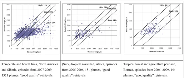
We considered only so-called “good” plume height trievals, for which the accuracy of the MISR plume-top re-trieval is the highest (Nelson et al., 2008; Val Martin et al., 2010). This selection reduces the size of the dataset from about 2500 fire cases down to 1650 cases, which is sufficient for the evaluation task.

The comparison of predictions of the formula (1) with MISR observations (Fig. 1) confirms (and strengthens) the main conclusion of the original evaluation by Sofiev et al. (2012). Formulation (1) proved to be robust and capa-ble of at least 70 % of predictions within 500 m of the

ob-servations (which is the accuracy of the MISR estimations themselves) in all conditions from boreal forests to tropical savannas. For Borneo, the fraction of good predictions was even higher at 94 %. The formula performance is further dis-cussed in Sect. 5.

3.2 Diurnal cycle of fire intensity

During the night, both fire intensity and turbulent mixing are suppressed, which leads to a reduction of the num-ber of active fires Nfires and mean FRP per active fire (FRPper-fire; Giglio, 2007; Roberts et al., 2009). The total regional energy release, FRPtotal=Nfires×FRPper-fire, de-creases even stronger, which corresponds to low nighttime emission. However, it is the diurnal cycle of FRPper-fire that drives the variation of the injection height. Reduction of FRPper-fire correlates with the nighttime stable atmospheric stratification and the low ABL height, leading to strong re-duction of the injection height.

Among the three above-mentioned fire-related quantities, only FRPtotal is observed by the satellites. Limited spatial resolution of even low-orbit (LEO) satellites (MODIS res-olution is 1–3 km), precludes them from seeing individual fires. For geostationary orbiting (GEO) instruments, such as SEVIRI, resolution is even worse: 10–30 km. Therefore, quantities actually measured from space are the number of overheated pixels (Nfire-pixels) and mean FRP of such pix-els (FRPper-pixel), and their relations withNfireand FRPper-fire are not fully established. Such aggregation is not the primary concern for the absolute emission fluxes, which are usually assumed to be linear to FRP, but it is a challenge for injection height calculations, where the dependence is non-linear.

Within this study, we do not aim to resolve the above un-certainty. Instead, we derive practically applicable estimates of diurnal cycles for both FRPtotal and FRPper-fire, which would be compatible with MODIS active-fire observations.

Estimating the diurnal cycles directly from MODIS FRP data is feasible only for high latitudes (Vermote et al., 2009). The typical four overpasses per day at low- and mid-latitudes, even if not obscured by clouds, are not sufficient to resolve the fire cycle (Ichoku et al., 2008). The only LEO satellite, which has more than 10 overpasses per day over equatorial regions, is TRMM with Visible and Infrared Scanner VIRS onboard. It provides only active-fire counts and thus can be used to estimate the diurnal cycle ofNfire-LEO-pixels, which is the closest available analogy toN_fires. Such an analysis has been reported by Giglio (2007).

The GEO instrument SEVIRI has sufficiently high tempo-ral resolution (∼15 min) and has been used to estimate the diurnal variations of FRPtotal and FRPper-GEO-pixel (Roberts and Wooster, 2008; Roberts et al., 2009).

(5)

Low: 19% High: 11%

Good: 70%

0 500 1000 1500 2000 2500 3000 3500 4000

Observed height, m

Cal

cul

ated

heig

ht,

m

Low: 11% High: 21%

Good: 68%

0 500 1000 1500 2000 2500 3000 3500 4000

Ca

lcul

at

ed

hei

g

ht,

m

Good: 94% High: 3%

0 500 1000 1500 2000 2500

Ca

lc

u

late

d

hei

g

h

t,

m

Temperate and boreal fires, North America

and Siberia, episodes from 2007-2009,

1321 plumes, “good quality” retrievals.

(Sub-) tropical savannah, Africa, episodes

from 2005-2006, 181 plumes, “good

quality” retrievals

Tropical forest and agriculture peatland,

Borneo, episodes from 2006- 2009, 144

plumes, “good quality” retrievals.

Fig. 1.Global evaluation of plume-top formulations of Sofiev et al. (2012) against MISR data. Unit=[m].

scatter in the data are too high. However, the dynamic range of the variation ofNfire-LEO-pixelreported for VIRS by Giglio (2007) and cycles of FRPtotaland FRPper-GEO-pixelcomputed for SEVIRI by Roberts et al. (2009) and Vermote et al. (2009) appeared compatible, thus suggesting that SEVIRI-based variations of FRPtotal FRPper-GEO-pixel are sufficient for the present study.

Since the above works included only qualitative presen-tations of the variations, we had to recompute them. Calcu-lations were made using SEVIRI data for a complete year, 2010, for three different land-use types: forest, grass, and mixed (compiled based on land-use maps of the US Geo-logical Survey, USGS). The normalised diurnal variations

Mtotal and Mper-GEO-pixel for FRPtotal and FRPper-GEO-pixel were modelled using truncated Fourier series with the co-efficientsak,bkfit into SEVIRI total and per-pixel FRP data

over the whole observed domain, separately for different land use typesl:

M•(nt, l)=a₀•+

3 X

k=1

a_k•(l)·cos

_k

12π nt

+

3 X

k=1

b_k•(l)

·sin

_k

12π nt

. (3)

Here,nt is an hour of the day,l is a land-use type, sign “•”

denotes “total” or “per-GEO-pixel” labels, and the Fourier coefficientsak,bk are obtained by fitting this model to the

SEVIRI FRP data. The obtained Fourier coefficients are pre-sented in Table 1 and the diurnal cycles are shown in Fig. 2.

As seen from Fig. 2, the diurnal cycle of FRPtotal is a single-peak curve, the dynamic range of which exceeds a fac-tor of 20. In contrast, FRPper-GEO-pixel exhibits several ups and downs with a very modest range of variation – a factor of 2. The small peaks in the morning and in the evening, as well as the local minima next to them, are not the artefacts of the Fourier processing but seem to represent the varying number of fires. Indeed, when fires are just starting in the

morning or dying out in the evening, the mean FRPper-pixelis small, which corresponds to the minima around 08:00 and 17:00 LT. But when the daytime fires are out, the number of fires reduces with only powerful events, which survive through night, remain visible for the satellite. Then the mean FRPper-GEO-pixelincreases again.

In the computations, we used the FRPtotaldiurnal cycle to simulate the variation of bulk-emission fluxes, whereas the FRPper-GEO-pixel cycle is used for the injection height. Each of the three land-use types was considered separately.

3.3 Gap filling

Apart from regions with regular fire events, there are many areas where few or no fires took place during some months of the analysed 12 years (Fig. 3). This leads to patchiness of the maps, which is inconvenient from a practical standpoint: some emission inventories are based on modelled fire prob-ability or external fire inventories, which are not constrained with fires registered by MODIS. Therefore, a gap-filling pro-cedure was applied to the cells, which had no fires reported for the specific month but had at least 3 out of 8 neighbour-ing cells with valid profiles:Nvalid ≥3. Then the profile in the empty cell (ie,je)for the monthme is computed as a linear combination of the valid neighbouring ones (in,jn), weighted with the number of firesNfnin each of them:

e(ie, je, k, me, d)=

Nvalid P

n=1

e(in, jn, k, me, d)Nfn(in, jn, me)

Nvalid P

n=1

Nfn(in, jn, me)

,

k=1, K (4)

(6)

Table 1.Fourier coefficients for FRP diurnal variation obtained from spectral analysis of SEVIRI data.

a0 a1 a2 a3 b1 b2 b3

Total FRP

Grass, 2010 1.000 −0.970 0.415 −0.143 −0.592 0.397 −0.196 Mixed, 2010 1.000 −1.288 0.631 −0.223 −0.673 0.605 −0.357 Forest, 2010 1.000 −1.180 0.587 −0.296 −0.740 0.598 −0.380

Mean FRP per pixel

Grass, 2010 1.000 −0.214 0.140 −0.084 −0.112 0.023 −0.016 Mixed, 2010 1.000 −0.198 0.162 −0.090 −0.129 0.014 −0.003 Forest, 2010 1.000 −0.041 0.141 −0.145 −0.119 0.037 −0.021

0 0.5 1 1.5 2 2.5 3 3.5 4

0 3 6 9 12 15 18 21

hr

Tot

a

l FR

P

v

a

ria

ti

o

n

grass, 2010 mixed, 2010 forest, 2010

0.6 0.8 1 1.2 1.4

0 3 6 9 12 15 18 21

hr

Me

a

n

FR

P

pe

r

p

ix

e

l v

a

ria

ti

on

grass, 2010 mixed, 2010 forest, 2010

a) b)

Fig. 2.Diurnal variations of total FRP (left), mean FRP per GEO-pixel (right). SEVIRI, mean over 2010. Relative unit.

the filled maps but both products, with and without gap-filling, are available for the users.

4 Results

The results of the computations consist of monthly nor-malised 3-D distributions of the total fire emission over the globe, separately for day- and nighttime, with and without gap filling (available at http://is4fires.fmi.fi).

A spatial pattern of injection heights appeared to be com-paratively homogeneous at a regional level but differences between the regions are large. There were also very strong diurnal and significant seasonal variations (Fig. 4).

The highest plumes are predicted for forested regions of North America (Rocky Mountains), parts of the Middle East to the south of the Caspian Sea, and Australia. During local summer season in these regions, the 90th percentile of a mass injection profile can exceed 3 km (i.e., 90 % of mass is emit-ted inside the layer spanning from the surface up to>3 km). Interestingly, these are not the regions where most of fires oc-cur. However, fires in Rocky Mountains, albeit not very fre-quent, are powerful, thus capable of sending the smoke high. In Australia, the fires are also powerful, whereas the high in-jection is additionally promoted by deep ABL. Conversely,

in the Middle East and Caspian region the reason may be a presence of numerous oil refineries, where powerful and persistent flames are partly misinterpreted as fires (see also discussion in Kaiser et al., 2012).

Regions with moderately high injection are forests in Amazonia and equatorial Africa, as well as grasses in south-ern Africa and central Eurasia. There, the 90th percentile is generally confined within 2.5 km. This outcome is not very surprising: these are regions known for quite strong fires and deep boundary layers (Ichoku et al., 2008b; van der Werf et al., 2010).

Among the regions with generally low injection, one can mention densely populated regions in all continents. There, the fires are probably better controlled and thus do not reach the strength needed to send the smoke high up into the at-mosphere. Interestingly, the infamous extremely high plumes from Siberian and Alaskan fires did not manifest themselves even in 90th percentile map (although these regions are in-deed characterised with high smoke injection). They were overshadowed by numerous moderate episodes that are much more frequent and responsible for the bulk of annual emis-sion. The second possible factor is a tendency of formula (1) to understate the elevation of high plumes (Fig. 1).

(7)

Fig. 3.Number of fires in February (left) and August (right) recorded by MODIS, sum from March 2000 until November 2012.

a) b)

c) d)

Fig. 4.Injection height for 90 % of mass for night (left) and day (right) for February (top) and August (bottom). Unit=[m].

injections occur during local summer, whereas fires in tropi-cal regions mainly occur during the dry season. In equatorial Africa, it is February to the north of equator and August to the south of it.

In general, the above results agree with common-sense ex-pectations that the strong fires are more probable in the ar-eas with the highest fuel load, strong droughts, and poor for-est and fire management. A zonally averaged vertical pro-file (Fig. 5) shows a similar picture: in the equatorial re-gion, where the bulk of contribution is from comparatively wet equatorial forests (predominantly man-made deforesta-tion fires), the top of the injecdeforesta-tion profile is lower than in the drier middle latitudes. One can also see that, despite record-high fires may reach up to 6 km, they have little impact on

the bulk of the emission: globally, more than 50 % of the fire emission is confined within the lowest 1–2 km, i.e. within the ABL. Both zonal averages and examples for a few regions in Fig. 5 show that the peak of emission during the daytime is attributed to the height range of 500 m–1 km, which receives up to 50 % of the total mass. The above-discussed differences in height of the 90th percentile are all due to comparatively limited differences in the mass fraction injected above this layer. This is also consistent with previous estimates (Kahn et al., 2008; Labonne et al., 2007; Sofiev et al., 2009; Val Martin et al., 2010).

(8)

Fig. 5.Mean regional average injection profiles: zonal average during the night, [m] (left), zonal average during the day, [m] (middle), injection profiles for some regions, daytime, August, [mass fraction as a function ofz] (right).

lead to low injection during the night, whereas stronger fires and deeper ABL during the day result in significantly higher injections. As a zonal mean, the bulk of emissions during the night is confined within 500 m, whereas during the day it spreads up to 1.5–2 km.

5 Discussion

5.1 Performance of the plume-top prediction formula

Evaluation of the plume-top formula (1) reported in Sect. 3.1 has confirmed high accuracy of the approach but also high-lighted the tendency of the parameterisation to over-estimate the height of low plumes and under-estimate it for high ones: the predicted heights have a lower dynamic range than the observed ones. For the African dataset this resulted in bias of∼150 m, owing to a significant fraction of over-estimated low plumes (Hp<700 m). For Borneo, where the fires were more powerful (but not too strong) and plumes generally went from 700 m to 1.5 km, the agreement was very good: the bias was less than 30 m and>90 % of the plumes were predicted within 500 m of the observations. Good agreement was also facilitated by the absence of high plumes, e.g. above 3 km, which are poorly reproduced by our approach (e.g., the left-hand panel for Siberian and US datasets).

A potential explanation of this tendency is missing de-pendence on the fire area. Thus, grass fires usually occupy wide areas, so that the FRP density, [W m−2_{], is} substan-tially lower than that for the forest fires, despite the fact that total FRP can be comparable. The present formula does not take this into account due to the high uncertainty of the fire area estimations derived from satellite data and practically unknown fire shape (position of the fire fronts, temperature distribution over the burn area, etc.). As a result, predicted plume top for a wide but low-FRP-density fire will be the same as that for a concentrated limited-area event –

provid-ing that the total FRPs and meteorological conditions are the same. In reality, one might expect the plume from a concen-trated fire to be injected higher. Similar dependence of the plume injection height on the fire area was noticed by Raf-fuse et al. (2012), who used the Briggs formula and faced severe difficulties evaluating very wide fires in the north-western US.

A possible workaround against the under-estimation of high plumes was suggested by Sofiev et al. (2012) in the form of a two-step procedure, which treats free-troposphere plumes separately from those in ABL. Its scores, being ex-tremely good for FT-plumes, however, suffer from misclas-sification of ABL/FT plume location. Therefore, we did not use it here.

The other uncertainty of the approach is connected with a time period needed for the plume to reach its top position. The formula (1) was calibrated using MISR plume-top data and MODIS FRP for the same fires. Since MISR is onboard the same Terra satellite as MODIS, their observations are per-formed simultaneously. However, the observed plume was actually formed by the smoke released from the fire some 15–30 min before the overpass (this is a rough estimate of time needed for a fire plume to reach its highest elevation). In the morning and evening hours, it can lead to up to 20–30 % of difference in the FRP value (if estimated from the diur-nal variation shown in Fig. 2 and Table 1). Consequently, the height of the plume should also be related to the past-time FRP. It can bring a few tens of metres of difference to the

H_pprediction, thus affecting the formula calibration. Finally, the uncertainties of ABL height determination and FRP re-trievals also contribute to the gross error.

(9)

Fig. 6.The 90th percentile of the aerosol profiles observed by the CALIOP lidar, February (left, data 2007–2012) and August (right, data 2006–2012). Daytime. Unit: [km].

one considers physical processes, rather than geographical locations, the dataset is very good and can be considered as representative for global applications. Indeed, in terms of meteorology, a wide range of conditions from strong tropi-cal convection to stable stratification at high latitudes are all represented. With regard to fires, it includes events in dense forests, mixtures of sparse forests and grassland, savannas, and tropical jungles. Sofiev et al. (2009) compared the distri-bution of FRP for fires, the plumes of which were analysed by MISR, with the full set of MODIS. They found that the MISR dataset includes a somewhat larger fraction of strong fires but still covers practically the whole range of the fire intensity observed by MODIS. Probably the only missing component is huge fires with extremely high energy release, where pyroconvection is the primary factor controlling the plume rise. For such events, formula (1) should be applied with great care or replaced with explicit modelling of dy-namics of the highly buoyant plumes.

5.2 Comparison of profiles with CALIOP observations

The CALIOP monthly vertical profiles of aerosols (CALIPSO, 2011), presently covering the period 2006– 2012, provide arguably the only reference dataset for evaluation of mean fire injection heights. However, direct comparison between the profiles obtained in the current work and the CALIOP observations is not possible because (i) CALIOP observes less than 3 % of the Earth’s surface and its overpasses are infrequent, (ii) it cannot distinguish between fresh and aged plumes, (iii) the detection of aerosol type is not accurate and, (iv) in particular, it assumes that only elevated aerosol clouds can be the fire smoke (Omar et al., 2009). One of the consequences of these issues is that the mean fire-attributed plumes are “shifted” upwards due to the cut-off of their lower parts. However, the upper percentiles of injection height can still be compared over regions with widespread fires: they are not too sensitive to the cut-off of the low plumes.

Comparison of the 90th percentile of plume mass injec-tion of this study (Fig. 4, right-hand panels) and the 90th percentile of CALIOP (Fig. 6) showed generally good

agree-ment, with our estimates being slightly lower than those es-timated by CALIOP.

In February (Fig. 6a), CALIOP observations in southern Europe show the majority of the plumes below 1 km, which is the same range as in the present study (Fig. 4b). In south-east Asia, the height varies. A typical level is about 1.5 km over the bulk of the area (current study suggests 1–1.5 km, see Fig. 4b) but up to 3 km is suggested over industrial regions of China, which is not reproduced by the current study (Fig. 4b). It is, however, unclear how such strong fires can show up in densely populated and highly cultivated and industrialised regions. Possibly, a mis-attribution of anthropogenic PM and wind-blown dust to fires can be a plausible explanation. Sur-prisingly, no fire plumes were recognised by CALIOP in equatorial Africa, whereas in the south their density is dispro-portionately large compared to that of active fires: the main fire season there is June–September, not February. These in-consistencies are probably again due to incorrect attribution of the observed plumes. The pattern in southern Africa qual-itatively agrees with our results: the 90th percentile of the plumes is between 1 km and 2.5 km with downward trend towards the coast. Finally, observations in equatorial South America suggest about 1–1.5 km typical height, in agreement with the current predictions.

Comparison of the patterns for August is more homoge-neous: plumes in Amazonia, southern Africa, southern Eu-rope, eastern US and south-east Asia, are well represented in the CALIOP dataset and the patterns are less noisy. As in February, the ranges are similar to the present study, with a tendency to show somewhat higher elevations than predicted – by a few hundred metres.

(10)

et al. (2011) for estimates of the smoke export from the con-tinent).

The impact of aged plumes made evaluation of the night-time profiles meaningless: CALIOP did not record any sig-nificant difference compared to the daytime. In several re-gions, the nighttime plumes were even higher than during the day. This is not surprising: the fire emission during the day is 10–20 times stronger than during the night, so the previous-day plumes recorded at night easily overshadow the fresh smoke and hide the actual position of the newly released plumes.

5.3 Comparison of 90 % map and zonal averages with

AEROCOM

We are aware of only one global, spatially resolving map of mean injection top: the one recommended for the AE-ROCOM (Aerosol Comparisons between Observations and Models) modelling community by Dentener et al. (2006). In that work, the authors assigned certain release profiles to the specific land-use types (see Table 4, Dentener et al., 2006) and suggested the maximum release height map (see Fig. 9 of Dentener et al., 2006). Unfortunately, it is not clear how those profiles and maximum heights were obtained.

The suggested AEROCOM maximum heights can be re-lated to our upper percentile maps (Fig. 4), whereas the pro-files of Table 4 of Dentener et al. (2006) can, to some extent, be related to the zonal average (Fig. 5). Such a comparison reveals similarities but also significant differences between the estimates.

Among the similarities, one can notice the western part of North America, where both datasets suggest quite high fires reaching 3 km. Agreement exists also over Oceania and parts of Australia, where the height of 90 % of the mass injection is close to the top height recommended for AEROCOM.

For South America the datasets show significantly differ-ent patterns: the currdiffer-ent assessmdiffer-ent has not registered high plumes over the eastern coast and in the south, instead re-porting them in the forest regions in the middle of the conti-nent, in agreement with CALIOP observations. The number of fires follows this trend too (Fig. 3). Such a pattern is to be expected since in densely populated coastal regions the fires are controlled more tightly than in tropical forest, whether or not they are set deliberately. As a result, the fire strength should be lower in the more densely populated regions.

Patterns over Eurasia and Australia differ strongly. The highest plumes in the AEROCOM map are over semi-desert areas of Australia and tundra in northern Eurasia, where MODIS registered just a few small fires. These regions are also characterised by a limited amount of fuel available for quick consumption and, in the case of northern Eurasia, fre-quent occasions of shallow ABL even during summer (Bak-lanov and Grisogono, 2007). Therefore, it seems unlikely to have high plumes over these regions, in agreement with our calculations.

5.4 Diurnal and seasonal variations of the injection profiles

Diurnal variation of the injection height is huge (Figs. 4, 5): one can practically consider two independent datasets – one for daytime and one for nighttime, with transition during morning and evening.

Apart from the diurnal variations, the seasonal changes of the injection profile are also important: as our analysis showed, both FRP and ABL height follow quite similar sea-sonality with peaks in dry hot months. As a result, the mean height of the 90th percentile of the injection profiles shows seasonal variation of about 30–40 %. This result is in quali-tative agreement with Val Martin et al. (2010) estimates for North America.

5.5 Impact of inhomogeneous meteorological data

The current study used operational meteorological data of ECMWF, which keeps developing its model and periodically updates the operational version. Since 2000, its horizontal and vertical resolutions have increased, the amount of assim-ilated observational information has grown manifold, several modules were updated, etc. More homogeneous would be the ERA-Interim dataset (Dee et al., 2011), which has con-stant resolution and a model version. However, it has several drawbacks: (i) it is still not completely homogeneous since the assimilated data vary, (ii) it has lower vertical resolu-tion than the operaresolu-tional model (60 levels versus 91 levels starting from 2006). Therefore, we stick to the operational ECMWF data but used our own procedure, derivingH_ABL

from the basic meteorological parameters (temperature and wind speed profiles, see Sect. 2 .2.2), which was the same for all years. We also checked thatH_ABL andN_FT do not have trends and break-points that can be attributed to the changes in the ECMWF model. Arguably the most suspicious mo-ment in that respect is 2 February 2006 when the model ver-tical grid was changed from 61 to 91 levels, along with other modifications.

Since variations ofNFThave only minor effects on the in-jection height (Sofiev et al., 2012), below we present only the analysis of ABL height. Its variations between the sea-sons and years are illustrated via histograms calculated for each month using all terrestrial grid cells (Fig. 7).

(11)

February 1.00E+03 1.00E+04 1.00E+05 1.00E+06 1.00E+07 0-50 30 0-35 0 60 0-65 0 90 0-95 0 1 200 -125 0 1 500 -155 0 1 800 -185 0 2 100 -215 0 2 400 -245 0 2 700 -275 0 3 000 -305 0 3 300 -335 0 3 600 -365 0 3 900 -395 0 4 200 -425 0 4 500 -455 0 4 800 -485 0 ABL N -ca se s 2001 2002 2003 2004 2005 2006 2007 2008 2009 2010 2011 2012 August 1.00E+03 1.00E+04 1.00E+05 1.00E+06 1.00E+07 0-50 30 0-35 0 60 0-65 0 90 0-95 0 1 200 -125 0 1 500 -155 0 1 800 -185 0 2 100 -215 0 2 400 -245 0 2 700 -275 0 3 000 -305 0 3 300 -335 0 3 600 -365 0 3 900 -395 0 4 200 -425 0 4 500 -455 0 4 800 -485 0 ABL N -ca se s 2001 2002 2003 2004 2005 2006 2007 2008 2009 2010 2011 2012

February zoom low-ABL

1.00E+05 6.00E+05 1.10E+06 1.60E+06 2.10E+06 2.60E+06 0-5 0 50 -1 00 100 -15 0 150 -20 0 200 -25 0 250 -30 0 300 -35 0 350 -40 0 400 -45 0 450 -50 0 500 -55 0 550 -60 0 600 -65 0 650 -70 0 ABL N -c ase s 2001 2002 2003 2004 2005 2006 2007 2008 2009 2010 2011 2012

August, zoom low-ABL

1.00E+05 4.00E+05 7.00E+05 1.00E+06 1.30E+06 1.60E+06 1.90E+06 2.20E+06 0-5 0 50 -1 00 100 -15 0 150 -20 0 200 -25 0 250 -30 0 300 -35 0 350 -40 0 400 -45 0 450 -50 0 500 -55 0 550 -60 0 600 -65 0 650 -70 0 ABL N -c ase s 2001 2002 2003 2004 2005 2006 2007 2008 2009 2010 2011 2012

Fig. 7.Histograms of ABL over land, February (left), August (right). Lower row shows the same charts as the upper one, zoomed for low ABL heights.

Fig. 8.Inter-annual variability of monthly profiles. Maps of lowest (left) and highest (right) monthly injection top heights for the 90 % of mass, min/max over 2000–2012. August, daytime. Unit=[m].

rather than systematic model changes. A similar effect is seen from the zoom over shallow ABLs: the highest fraction of

HABL<150 m was in 2009 and 2010, whereas the lowest one – in 2006;; all three were derived from the data with 91 vertical levels.

Histograms in August are barely distinguishable between the years, with some difference showing up only for the thickest ABLs. And again, no regular pattern or any rela-tion to the vertical resolurela-tion change in 2006 was found. Therefore, we conclude that the meteorological input of the study does not have significant trends or break-points due to changes in the ECMWF meteorological model.

5.6 Representativeness of the obtained profiles for specific applications

The current profiles have been obtained from the analysis of over 12.5 yr – from March 2000 till November 2012. These include all available to-date FRP data from MODIS and pro-vide the best possible coverage ensuring that no fire-prone region is missing from the maps (Figs. 3, 4). Still, the num-ber of fire events for specific months can be fewer than 10 for some grid cells (Fig. 3). For these areas the results of the current computations should be taken with care.

(12)

fire is mandatory, possibly, with the two-step procedure sug-gested by Sofiev et al. (2012).

At a monthly level, representativeness of the results is bet-ter but year-to-year variability is still significant. The related uncertainty can be qualitatively illustrated by comparing the lowest and the highest positions of the 90th monthly per-centile among the considered years. Such maps were com-piled in Fig. 8, where each grid cell represents the lowest (panel a) and the highest (panel b) position of the 90th per-centile in August among all considered years. Similar maps for all months are available together with the main dataset at http://is4fires.fmi.fi.

6 Summary

The presented dataset is the result of bottom-up computations of characteristic vertical profiles of smoke from wildland fires. It is obtained by processing records of active fires of MODIS instruments onboard Aqua and Terra satellites. The analysis was made for daytime and nighttime separately, cov-ered all years available to date from MODIS (2000–2012), extended over the whole globe, and resulted in monthly 3-D maps of injected fraction of fire smoke.

The computations showed that the highest plumes reach-ing up to 6 km are characteristic for forested areas, whereas grassland fires usually emit within the lowest 2–3 km. How-ever, 90 % of mass is emitted within∼3 km layer, if the long-term average is considered.

Strong diurnal and seasonal variations of the injection pro-files were found all over the globe. It is therefore recom-mended to account for these variations in practical applica-tions.

Comparison with the independent CALIOP observations showed high similarity of the patterns. Somewhat higher al-titude of the 90th percentile obtained by the lidar (few hun-dreds of metres) could originate from the impact of aged plumes dispersed over thick layers and recorded by lidar to-gether with the fresh smoke from the fires.

Comparison with AEROCOM recommendations showed both similarities and differences between the injection height maps. However, in most cases the results of the current study seem to be more logical and supported by CALIOP data, es-pecially in the areas with significant seasonal variations of the injection height.

Noticeable inter-annual variation suggests that a dynamic evaluation of emission from each specific fire, if it appears possible, would bring about more accurate estimates, espe-cially if a limited-time regional episode is concerned. The current dataset is mostly useful for long-term global and con-tinental studies, where an analysis of each individual fire is unfeasible.

The dataset is publicly available at http://is4fires.fmi.fi.

Acknowledgements. The study has been performed within the ESA

GlobEmission and TEKES KASTU 2 projects. Support of EU FP7 PASODOBLE and PEGASOS, Academy of Finland ASTREX and Russian projects “Conducting of problem-oriented research in monitoring technologies and forecasting of atmospheric state in forest and peat fire” and “Grant to research projects implemented under the supervision of the worlds leading scientists (contract No. 11.G34.31.0078)” is kindly acknowledged. Discussions with MACC and AEROCOM fire assessment teams are highly appreciated. The MODIS, MISR and CALIOP satellite data were obtained from public online data banks of NASA. MSG SEVIRI data were archived from the ENVISAT dissemination service.

Edited by: S. Kloster

References

Baklanov, A. and Grisogono, B.: Atmospheric boudnary layers. Na-ture, theory, and application to environmental modelling and se-curity, Springer, Dubrovnik, 2007.

Briggs, G. A.: Plume rise predictions, in Lectures on air pollution and environmental impact analyses, 59–111, Boston, 1975. CALIPSO: CALIPSO Quality Statements Lidar Level 3 Aerosol

Profile Monthly Products Version Release: 1.00, 2011.

Davison, P. S.: Estimating the direct radiative forcing due to haze from the 1997 forest fires in Indonesia, J. Geophys. Res., 109, 1–12, doi:10.1029/2003JD004264, 2004.

Dee, D. P., Uppala, S. M., Simmons, A. J., Berrisford, P., Poli, P., Kobayashi, S., Andrae, U., Balmaseda, M. A., Balsamo, G., Bauer, P., Bechtold, P., Beljaars, A. C. M., van de Berg, L., Bid-lot, J., Bormann, N., Delsol, C., Dragani, R., Fuentes, M., Geer, A. J., Haimberger, L., Healy, S. B., Hersbach, H., Hólm, E. V., Isaksen, L., K˚allberg, P., Köhler, M., Matricardi, M., McNally, A. P., Monge-Sanz, B., M. Morcrette, J.-J., Park, B.-K., Peubey, C., de Rosnay, P., Tavolato, C., Thépaut, J.-N., and Vitart, F.: The ERA-Interim reanalysis: configuration and performance of the data assimilation system, Q. J. Roy. Meteorol. Soc., 137, 553– 597, doi:10.1002/qj.828, 2011.

Dentener, F., Kinne, S., Bond, T., Boucher, O., Cofala, J., Generoso, S., Ginoux, P., Gong, S., Hoelzemann, J. J., Ito, A., Marelli, L., Penner, J. E., Putaud, J.-P., Textor, C., Schulz, M., van der Werf, G. R., and Wilson, J.: Emissions of primary aerosol and precur-sor gases in the years 2000 and 1750 prescribed data-sets for Ae-roCom, Atmos. Chem. Phys., 6, 4321–4344, doi:10.5194/acp-6-4321-2006, 2006.

Dirksen, R. J., Folkert Boersma, K., de Laat, J., Stammes, P., van der Werf, G. R., Val Martin, M., and Kelder, H. M.: An aerosol boomerang: Rapid around-the-world transport of smoke from the December 2006 Australian forest fires observed from space, J. Geophys. Res., 114, 1–15, doi:10.1029/2009JD012360, 2009. Fiedler, V., Arnold, F., Ludmann, S., Minikin, A., Hamburger,

T., Pirjola, L., D¨ornbrack, A., and Schlager, H.: African biomass burning plumes over the Atlantic: aircraft based mea-surements and implications for H₂SO₄ and HNO₃ mediated smoke particle activation, Atmos. Chem. Phys., 11, 3211–3225, doi:10.5194/acp-11-3211-2011, 2011.

(13)

pre-processing of meteorological data for atmospheric dispersion models, edited by: Fisher, B. E. A., Erbrink, J. J., Finardi, S., Jeannet, P., Joffre, S., Morselli, M. G., Pechinger, U., Seibert, P., and Thomson, D.: Office for Official Publications of the Euro-pean Communities, Luxembourg, available from: http://www2. dmu.dk/atmosphericenvironment/cost/FinalRep.htm, 1998. Forster, C. Wandinger, U. Wotawa, G., James, P., Mattis, I,

Althausen, D., Simmonds, P., O’Doherty, S., Jennings, S. G., Kleefeld, C., Schneider, J., Trickl, T., Kreipl, S., J¨ager, H., and Stohl, A.: Transport of boreal forest fire emissions from Canada to Europe, J. Geophys. Res., 106, 22887–22906, doi:10.1029/2001JD900115, 2001.

Freeborn, P. H., Wooster, M. J., Hao, W. M., Ryan, C. A., Nord-gren, B. L., Baker, S. P., and Ichoku, C.: Relationships between energy release, fuel mass loss, and trace gas and aerosol emis-sions during laboratory biomass fires, J. Geophys. Res., 113, 1– 17, doi:10.1029/2007JD008679, 2008.

Freitas, S. R., Longo, K. M., Chatfield, R., Latham, D., Silva Dias, M. A. F., Andreae, M. O., Prins, E., Santos, J. C., Gielow, R., and Carvalho Jr., J. A.: Including the sub-grid scale plume rise of veg-etation fires in low resolution atmospheric transport models, At-mos. Chem. Phys., 7, 3385–3398, doi:10.5194/acp-7-3385-2007, 2007.

Fromm, M., Jerome, A., Hoppel, K., Hornstein, J., Bevilacqua, R., Shettle, E., Servranckx, R., Zhanqing, L., and Stocks, B.: Obser-vations of boreal forest fire smoke in the stratosphere by POAM III, SAGE II, and lidar in 1998, Geophys. Res. Lett., 27, 1407– 1410, doi:10.1029/1999GL011200, 2000.

Giglio, L.: Characterization of the tropical diurnal fire cycle using VIRS and MODIS observations, Remote Sens. Environ., 108, 407–421, doi:10.1016/j.rse.2006.11.018, 2007.

Ichoku, C., Giglio, L., Wooster, M. J., and Remer, L. A.: Global characterization of biomass-burning patterns using satellite mea-surements of fire radiative energy, Remote Sens. Environ., 112, 2950–2962, doi:10.1016/j.rse.2008.02.009, 2008a.

Ichoku, C., Giglio, L., Wooster, M. J., and Remer, L. A.: Global characterization of biomass-burning patterns using satellite mea-surements of fire radiative energy, Remote Sens. Environ., 112, 2950–2962, doi:10.1016/j.rse.2008.02.009, 2008b.

Justice, C. O., Giglio, L., Korontzi, S., Owens, J., Morisette, J. T., Roy, D., Descloitres, J., Alleaume, S., Petitcolin, F., and Kauf-man, Y.: The MODIS fire products, Remote Sens. Environ., 83, 244–262, 2002.

Kahn, R. A., Chen, Y., Nelson, D. L., Leung, F.-Y., Li, Q., Diner, D. J., and Logan, J. A.: Wildfire smoke injection heights: Two perspectives from space, Geophys. Res. Lett., 35, 4–7, doi:10.1029/2007GL032165, 2008.

Kaiser, J. W., Wooster, M. J., Roberts, G., Schultz, M. G., Van Der Werf, G., and Benedetti, A.: SEVIRI Fire Radiative Power and the MACC Atmospheric Services, in EUMETSAT Meteorologi-cal Satellite Conf., ISBN 978-92-9110-086-6, ISSN 1011-3932, 2005–2009, EUMETSAT, Darmstadt, Germany, 2009.

Kaiser, J. W., Heil, A., Andreae, M. O., Benedetti, A., Chubarova, N., Jones, L., Morcrette, J.-J., Razinger, M., Schultz, M. G., Suttie, M., and van der Werf, G. R.: Biomass burning emis-sions estimated with a global fire assimilation system based on observed fire radiative power, Biogeosciences, 9, 527–554, doi:10.5194/bg-9-527-2012, 2012.

Kaufman, I., Steele, M., Cummings, D. L., and Jaramillo, V. J.: Biomass dynamics associated with deforestation, fire, and, con-version to cattle pasture in a Mexican tropical dry forest, Forest Ecol. Manage., 176, 1–12, 2003.

Kaufman, Y. J., Justice, C. O., Flynn, L. P., Kendall, J. D., Prins, E. M., Giglio, L., Ward, D. E., Menzel, W. P., and Setzer, A. W. (1998), Potential global fire monitoring from EOS-MODIS, J. Geophys. Res.-Atmos., 103, 32215–21238, 1998.

Kouznetsov, R., Wood, C., Soares, J., Sofiev, M., Karppinen, A., and Fortelius, C.: Sodar verification for boundary-layer height diagnostics in meteorological models, in Proc. 16-th Int. Symp. for the Advancement of Boundary Layer Remote Sensing (P01-7, 1–4). Boulder, CO., PO1–(P01-7, 1–4, Boulder, CO, 2012. Labonne, M., Br´eon, F.-M., and Chevallier, F.: Injection height of

biomass burning aerosols as seen from a spaceborne lidar, Geo-phys. Res. Lett., 34, 1–5, doi:10.1029/2007GL029311, 2007. Lavou´e, D., Liousse, C., Cachier, H., Stocks, B. J., and Goldammer,

J. G.: Modeling of carbonaceous particles emitted by boreal and temperate wildfires at northern latitudes, J. Geophys. Res., 105(D22), 26871–26890, doi:10.1029/2000JD900180, 2000. Liousse, C., Penner, J. E., Chuang, C., Walton, J. J., Eddleman,

H., and Cachier, H.: A global three-dimensional model study of carbonaceous aerosols, J. Geophys. Res., 101, 19411–19432, doi:10.1029/95JD03426, 1996.

Luderer, G., Trentmann, J., Winterrath, T., Textor, C., Herzog, M., Graf, H. F., and Andreae, M. O.: Modeling of biomass smoke injection into the lower stratosphere by a large forest fire (Part II): sensitivity studies, Atmos. Chem. Phys., 6, 5261–5277, doi:10.5194/acp-6-5261-2006, 2006.

Mazzoni, D., Logan, J. A., Diner, D., Kahn, R. A., Tong, L., and Li, Q.: A data-mining approach to associating MISR smoke plume heights with MODIS fire measurements, Remote Sens. Environ., 107, 138–148, 2007.

Nelson, D., Lawshe, C., Diner, D., and Kahn, R.: MISR Plume Height Project, Data Quality Statement and Error Analy-sis, 3, available from: http://www-misr.jpl.nasa.gov/getData/ accessData/MisrMinxPlumes/qualityStatement/, 2008.

Omar, A. H., Winkar, D. M., Kittaka, C., Vaughan, M. A., Liu,Z., Hu, Y., Trepte, C. R., Rogers, R. R., Ferrare, R. A., Lee, K.-P., Kuehn, R. E., Hostetler, C. A.: The CALIPSO Automated Aerosol Classification and Lidar Ratio Selec-tion Algorithm, J. Atmos. Ocean. Tech., 26, 1994–2014, doi:10.1175/2009JTECHA1231.1, 2009.

Raffuse, S. M., Craig, K. J., Larkin, N. K., Strand, T. T., Sul-livan, D. C., Wheeler, N. J. M., and Solomon, R.: An Eval-uation of Modeled Plume Injection Height with Satellite-Derived Observed Plume Height, Atmosphere, 3, 103–123, doi:10.3390/atmos3010103, 2012.

Rio, C., Hourdin, F., and Ch´edin, A.: Numerical simulation of tro-pospheric injection of biomass burning products by pyro-thermal plumes, Atmos. Chem. Phys., 10, 3463–3478, doi:10.5194/acp-10-3463-2010, 2010.

Roberts, G. J. and Wooster, M. J.: Fire Detection and Fire Char-acterization Over Africa Using Meteosat SEVIRI, IEEE Trans-actions on Geoscience and Remote Sensing, 46, 1200–1218, doi:10.1109/TGRS.2008.915751, 2008.

(14)

Sofiev, M., Siljamo, P., Valkama, I., Ilvonen, M., and Kukko-nen, J.: A dispersion modelling system SILAM and its eval-uation against ETEX data, Atmos. Environ., 40, 674–685, doi:10.1016/j.atmosenv.2005.09.069, 2006.

Sofiev, M., Vankevich, R., Lotjonen, M., Prank, M., Petukhov, V., Ermakova, T., Koskinen, J., and Kukkonen, J.: An operational system for the assimilation of the satellite information on wild-land fires for the needs of air quality modelling and forecasting, Atmos. Chem. Phys., 9, 6833–6847, doi:10.5194/acp-9-6833-2009, 2009.

Sofiev, M., Ermakova, T., and Vankevich, R.: Evaluation of the smoke-injection height from wild-land fires using remote-sensing data, Atmos. Chem. Phys., 12, 1995–2006, doi:10.5194/acp-12-1995-2012, 2012.

Stein, A. F., Rolph, G. D., Draxler, R. R., Stunder, B., and Rumin-ski, M.: Verification of the NOAA Smoke Forecasting System: Model Sensitivity to the Injection Height, Weather Forecast., 24, 379–394, doi:10.1175/2008WAF2222166.1, 2009.

Sukhinin, A. I., Conard, S. G., McRae, D. J., Ivanova, G. A., Tsvetkov, P. A., Bychkov, V. A., and Slinkina, O. A.: Remote Sensing of Fire Intensity and Burn Severity in Forests of Cen-tral Siberia, in Contemporary Problems of Earth Remote Sens-ing from Space, Space Research Institute RAS, Mscow, available from: http://www.iki.rssi.ru/earth/ppt2005/sukhinin.pdf, 2005. Tosca, M. G., Randerson, J. T., Zender, C. S., Nelson, D. L., Diner,

D. J., and Logan, J. A.: Dynamics of fire plumes and smoke clouds associated with peat and deforestation fires in Indone-sia, J. Geophys. Res., 116, D08207, doi:10.1029/2010JD015148, 2011.

Val Martin, M., Logan, J. A., Kahn, R. A., Leung, F.-Y., Nelson, D. L., and Diner, D. J.: Smoke injection heights from fires in North America: analysis of 5 years of satellite observations, At-mos. Chem. Phys., 10, 1491–1510, doi:10.5194/acp-10-1491-2010, 2010.

van der Werf, G. R., Randerson, J. T., Giglio, L., Collatz, G. J., Kasibhatla, P. S., and Arellano Jr., A. F.: Interannual variabil-ity in global biomass burning emissions from 1997 to 2004, At-mos. Chem. Phys., 6, 3423–3441, doi:10.5194/acp-6-3423-2006, 2006.

van der Werf, G. R., Randerson, J. T., Giglio, L., Collatz, G. J., Mu, M., Kasibhatla, P. S., Morton, D. C., DeFries, R. S., Jin, Y., and van Leeuwen, T. T.: Global fire emissions and the contribution of deforestation, savanna, forest, agricultural, and peat fires (1997– 2009), Atmos. Chem. Phys., 10, 11707–11735, doi:10.5194/acp-10-11707-2010, 2010.

Vaughan, M. A., Powell, K. A., Kuehn, R. E., Young, S. A., Winker, D. M., Hostetler, C. A., Hunt, W. H., Liu, Z., McGill, M. J., and Getzewich, B. J.: Fully Automated De-tection of Cloud and Aerosol Layers in the CALIPSO Li-dar Measurements, J. Atmos. Ocean. Tech., 26, 2034–2050, doi:10.1175/2009JTECHA1228.1, 2009.

Vermote, E., Ellicott, E., Dubovik, O., Lapyonok, T., Chin, M., Giglio, L., and Roberts, G. J.: An approach to estimate global biomass burning emissions of organic and black carbon from MODIS fire radiative power, J. Geophys. Res., 114, 1–22, doi:10.1029/2008JD011188, 2009.

Wang, J., Christopher, S. A., Nair, U. S., Reid, J. S., Prins, E. M., Szykman, J., and Hand, J. L.: Mesoscale modeling of Central American smoke transport to the United States: 1. “Top-down” assessment of emission strength and diurnal variation impacts, J. Geophys. Res., 111, 1–21, doi:10.1029/2005JD006416, 2006. Westphal, L. and Toon, O. B.: Simulations of Microphysical,

Ra-diative, and Dynamical Processes in a Continental-Scale For-est Fire Smoke Plume, J. Geophys. Res., 96, 22379–22400, doi:10.1029/91JD01956, 1991.