www.atmos-chem-phys.net/15/12397/2015/ doi:10.5194/acp-15-12397-2015
© Author(s) 2015. CC Attribution 3.0 License.
Putting the clouds back in aerosol–cloud interactions
A. Gettelman
National Center for Atmospheric Research, 1850 Table Mesa Dr., Boulder, CO 80305, USA
Correspondence to:A. Gettelman ([email protected])
Received: 17 July 2015 – Published in Atmos. Chem. Phys. Discuss.: 3 August 2015 Revised: 23 October 2015 – Accepted: 27 October 2015 – Published: 9 November 2015
Abstract. Aerosol–cloud interactions (ACI) are the conse-quence of perturbed aerosols affecting cloud drop and crys-tal number, with corresponding microphysical and radiative effects. ACI are sensitive to both cloud microphysical pro-cesses (the “C” in ACI) and aerosol emissions and propro-cesses (the “A” in ACI). This work highlights the importance of cloud microphysical processes, using idealized and global tests of a cloud microphysics scheme used for global cli-mate prediction. Uncertainties in key cloud microphysical processes examined with sensitivity tests cause uncertainties of nearly−30 to +60 % in ACI, similar to or stronger than uncertainties identified due to natural aerosol emissions (−30 to +30 %). The different dimensions and sensitivities of ACI to microphysical processes identified in previous work are analyzed in detail, showing that precipitation processes are critical for understanding ACI and that uncertain cloud life-time effects are nearly one-third of simulated ACI. Buffering of different processes is important, as is the mixed phase and coupling of the microphysics to the condensation and turbu-lence schemes in the model.
1 Introduction
Aerosols represent the largest uncertainty in our estimates of current anthropogenic forcing of climate (Boucher et al., 2013), limiting our ability to constrain the sensitivity of the current climate to radiative forcing. Aerosols affect climate through direct effects of absorption or scattering, and in-direct effects (Twomey, 1977) by changing the number of cloud drops and resulting complex microphysical interac-tions. Increased aerosol number concentrations are associ-ated with more cloud condensation nuclei (CCN) (Rosenfeld
et al., 2008; Twomey and Squires, 1959), leading to higher cloud drop number concentrations (Nc). The relationship be-tween aerosols and CCN is affected by a number of factors (Lohmann and Feichter, 2005), including the aerosol type and meteorological conditions. The result is a different pop-ulation of cloud droplets, depending on aerosol distribution and meteorology.
But that is only the beginning of aerosol effects on clouds. Cloud microphysics (the interactions of a distribution of cloud drops at the micro-meter scale) determines how much water precipitates, the amount of water remaining in the cloud, and the resulting population of cloud drops. In global modeling experiments, aerosol–cloud interactions (ACI) can be altered by the representation of cloud microphysical pro-cesses (the “C” in ACI) while the aerosol propro-cesses (“A”) re-main largely unchanged. Menon et al. (2002), Rotstayn and Liu (2005), Penner et al. (2006), Wang et al. (2012) and Get-telman et al. (2013) all looked at changes to autoconversion, while Posselt and Lohmann (2008) looked at changes to pre-cipitation.
ACI are typically quantified by the change in cloud radia-tive effect (Ghan et al., 2013). ACI occur most readily with liquid sulfate aerosol (H2SO4) derived from sulfur dioxide (SO2) assisting the formation of cloud droplets, thus increas-ing cloud drop numbers. Higher drop numbers affect cloud albedo (Twomey, 1977), and potentially also affect cloud lifetime and dynamics (Albrecht, 1989; Pincus and Baker, 1994). Cloud lifetime and dynamics effects are highly uncer-tain (Stevens and Feingold, 2009).
clouds interact with aerosols, assuming aerosols translated into cloud drop numbers based on fixed cloud dynamics and water content (Carslaw et al., 2013), largely ignoring the “C” in ACI. The cloud microphysical state, defined as the combi-nation of cloud liquid water path and drop number, deter-mines cloud microphysical (precipitation rates) and radia-tive properties. As a result, perturbations to this state from aerosols (ACI) may depend on the base state; i.e., the re-sponse of a cloud to a change in CCN may depend on the unperturbed CCN and resulting drop number.
In this work we quantify the sensitivity of ACI to cloud microphysics with detailed off-line tests and global sensitiv-ity tests of ACI with a cloud microphysics scheme. First, de-tailed off-line tests will isolate the different components of ACI in a cloud microphysics scheme; off-line tests will in-clude exploration of lifetime effects and microphysical pro-cess rates. Then global simulations will analyze the sen-sitivity of ACI to many different aspects of cloud micro-physics, including sensitivity to (1) activation, (2) precipi-tation, (3) mixed phase processes, (4) autoconversion treat-ment, (5) coupling to other parameterizations and (6) back-ground aerosol emissions. These processes have been high-lighted in previous studies.
The methodology is described in Sect. 2. Detailed off-line tests are in Sect. 3. Global results and sensitivity tests are in Sect. 4, and conclusions are in Sect. 5.
2 Methods
The double-moment (mass and number predicting), bulk cloud microphysics scheme described by Morrison and Get-telman (2008) (hereafter MG1) and GetGet-telman and Morrison (2015) (hereafter MG2) is used for this study. The scheme handles a variable number of droplets specified from an ex-ternal activation scheme (Abdul-Razzak and Ghan, 2000). It can also run with a fixed droplet and crystal number. The scheme is implemented both in an off-line idealized kine-matic driver (KiD) (Shipway and Hill, 2012), as well as in a general circulation model (GCM) – the Community Earth System Model (CESM) (Gettelman and Morrison, 2015). The susceptibility of an earlier version of the scheme to aerosols has been shown by Gettelman et al. (2013) to be similar to detailed models with explicit bin microphysics that represent more accurately the precipitation process (Jiang et al., 2010).
2.1 Off-line tests
To isolate and test the microphysics we use a simple one-dimensional off-line driver, the KiD (Shipway and Hill, 2012) with the same microphysical parameterization as used in the global model. We use a 1 s time step, 25 m vertical resolution and a 3 km vertical domain in KiD. In the off-line implementation, specified drop numbers are assumed. Here
we focus only on warm rain cases. We use several different cases for analysis. The basic case (warm 2 or W2) features multiple 2 ms−1updrafts over 2 h (Gettelman and Morrison, 2015; Shipway and Hill, 2012). We have examined three other cases as well, with notation following Gettelman and Morrison (2015). These cases represent some basic idealized clouds commonly used to evaluate cloud microphysical pro-cesses such as condensation, precipitation and evaporation. Case 1 (W1) is a single 2 ms−1updraft that decays in time (1 h). Case 3 (W3) features multiple updrafts that weaken over time. Case 7 (W7) has shallower updrafts of maximum 0.5 ms−1over 8 h. To assess the impact of aerosols, experi-ments are conducted with variable drop number from 10 to 2000 cm−3. This spans the range from pristine to very pol-luted conditions.
In off-line tests, we estimate first the cloud albedo, and then divide albedo (A) changes into contributions from (1) liquid water path (LWP), (2) cloud drop number concen-tration (Nc) and (3) cloud coverage (C). To estimate albedo (A) we make the assumption that
A=C·τ/(β+τ ), (1)
whereβ=6.8,τ =α·LWP5/6·Nc1/3andα=0.19 (Zhang et al., 2005, Eqs. 19–20). Strictly speaking the albedo should include a surface reflectance term, which over ocean would be(1−C)·Asfc, where for oceanAsfc=0.05. For these ide-alized cases we assumeAsfc=0. The change in albedo (dA) can then be represented as
1A= dA
dNc
1Nc+ dA
dLWP1LWP+ dA
dC1C+r . (2) C(cloud cover or cloud fraction) has one value for each sim-ulation.Nchas one specified value for each simulation and LWP is an average over the simulation period.r is a resid-ual. The changes are discrete differences between simula-tions with different specifiedNcfor each case.
The idealized one-dimensional kinematic driver is de-signed to test different microphysical schemes in the same framework. Results of such idealized off-line tests are qual-itatively useful for examining the relative importance of in-dividual processes for ACI. We use them for illustration, and will use global sensitivity tests of the full GCM for quantifi-cation.
2.2 Global sensitivity tests
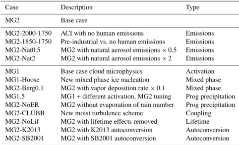
Table 1.Description of sensitivity tests used in the text, including the case short name (including the microphysics scheme used), a brief description, and the type of experiment. All tests are pairs of simulations as described in the text.
Case Description Type
MG2 Base case
MG2-2000-1750 ACI with no human emissions Emissions MG2-1850-1750 Pre-industrial vs. no human emissions Emissions MG2-Nat0.5 MG2 with natural aerosol emissions×0.5 Emissions MG2-Nat2 MG2 with natural aerosol emissions×2 Emissions
MG1 Base case cloud microphysics Activation
MG1-Hoose New mixed phase ice nucleation Mixed phase MG2-Berg0.1 MG2 with vapor deposition rate×0.1 Mixed phase MG1.5 MG1 + different activation, MG2 tuning Prog precipitation MG2-NoER MG2 without evaporation of rain number Prog precipitation
MG2-CLUBB New moist turbulence scheme Coupling
MG2-NoLif MG2 with lifetime effects removed Lifetime MG2-K2013 MG2 with K2013 autoconversion Autoconversion MG2-SB2001 MG2 with SB2001 autoconversion Autoconversion
For the global model, we run simulations with specified climatological sea surface temperatures (SSTs) and green-house gases representing year 2000 conditions. We then vary aerosol emissions in two simulations for the year 2000 and 1850; differences represent only the effects of aerosol emis-sions. 1850 refers only to the aerosol emissions greenhouse gases and SSTs remain at year 2000 conditions. Simulations are 1.9◦latitude by 2.5◦longitude horizontal resolution, they
are 6 years long, and the last 5 years are analyzed and are similar to previous work (Gettelman et al., 2012, 2015). Sen-sitivity tests are described below.
To understand the uncertainty in using 5 years of simu-lation, we performed an uncertainty analysis. This consisted of running the MG2 experiment out for 20 years (for 2000 and 1850 conditions). Analysis of separate 5-year periods indicates uncertainty of 0.08 Wm−2for ACI and long-wave (LW)/shortwave (SW) components (about 10 %) and within 0.04 Wm−2for direct effects relative to 20-year means. We also performed nudged experiments where winds or winds and temperatures were fixed to a previous CAM simulation, but these produced slightly different cloud radiative effects, and thus slightly different quantitative values for ACI (differ-ent by 20–40 %). Qualitative patterns and zonal mean struc-ture of ACI are similar to the free-running experiments.
In global simulations, ACI can be defined as the change in cloud radiative effects (CRE) in the LW and SW, where CRE are equal to the all sky top-of-atmosphere (TOA) radia-tive flux minus an estimate of what the clear-sky flux would be without clouds, but with the same state (temperature, hu-midity and surface structure). CRE are adjusted following Ghan et al. (2013) to use the “clean-sky” effects based on TOA fluxes estimated with a diagnostic call to the radiation code without aerosols. Results are similar, but with a slightly higher magnitude, to a direct estimate of ACI using CRE.
Di-rect absorption and scattering by aerosols is also estimated by differencing the TOA radiative fluxes to TOA fluxes es-timated with a diagnostic call to the radiation code without aerosols.
Table 1 describes the different sensitivity tests. As noted below, tests are motivated by previous studies identifying microphysical sensitivities. All tests are pairs of simulations with emissions of aerosols set to 2000 and 1850, except for the MG2-2000-1750 and MG2-1850-1750, which use differ-ent emissions years to explore differdiffer-ent magnitudes of sions changes. To explore how linear the changes in emis-sions are, we look at emisemis-sions without any human influence (no biomass burning, domestic or industrial emissions) and term this 1750. We also explore modifying background nat-ural emissions in both 1850 and 2000 by a factor of 0.5 or 2. These experiments test the impact of emissions (Carslaw et al., 2013), not cloud microphysics.
Tests also track the evolution of the cloud microphysics in CAM from MG1 (Morrison and Gettelman, 2008) to MG2 (Gettelman and Morrison, 2015). MG1.5 is an interim ver-sion that has (a) changes to the location where activated num-bers are applied to before estimation of microphysical pro-cesses (which thickens the stratiform clouds) and (b) com-pensating increases in the threshold relative humidity for cloud formation to thin clouds back to radiative balance. The difference between MG1 and MG1.5 tests the changes to the activation scheme. The impact of prognostic precipitation is tested by the differences between MG2 and MG1.5.
A) W2 Cloud Mass
0.0 0.2 0.4 0.6 0.8 1.0 1.2 1.4
cloud_mass (g/kg) 0
1000 2000 3000
Z (m)
B) W2 Surface Rain Rate
0 2000 4000 6000 8000
Time (s) 0.000
0.005 0.010 0.015
total_surface_ppt (mm hr-1)
Nc=10
Nc=20 Nc=50
Nc=100
Nc=200 Nc=500
Nc=1000 Nc=2000
C) W2 Rain Mass
0.00 0.05 0.10 0.15
rain_mass (g kg-1) 0
1000 2000 3000
Z (m)
D) W2 Albedo
0 2000 4000 6000 8000
Time (s) 0.0
0.2 0.4 0.6 0.8 1.0
Albedo
E) W2 Autoconversion Rate
0 5.0×10⁻⁸ 1.0×10⁻⁷ 1.5×10⁻⁷ 2.0×10⁻⁷
autoconversion_rate (kg kg-1 s-1) 0
1000 2000 3000
Z (m)
F) W2 Accretion Rate
0 1×10⁻⁷ 2×10⁻⁷ 3×10⁻⁷ 4×10⁻⁷ 5×10⁻⁷ 6×10⁻⁷
accretion_rate (kg kg-1 s-1) 0
1000 2000 3000
Z (m)
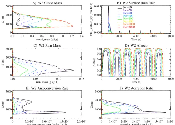
Figure 1.Warm 2 (W2) off-line tests of(a)time-averaged cloud mass (g kg−1),(b)time series of surface rain rate (mm h−1),(c) time-averaged rain mass (g kg−1),(d)time series of albedo, time-averaged(e)autoconversion and(f)accretion rates (kg kg−1s−1). Different colors correspond to different fixed cloud drop number concentrations.
vapor deposition process by a factor of 10. This sensitivity test is motivated by the work of Korolev (2007) and Korolev (2008), who suggested that due to updraft rates in clouds at least half the time the vapor deposition rate may not apply. It is also motivated by tests in Lawson and Gettelman (2014) extending this to a large-scale model that would also assume inhomogeneity in a grid box, and found improvements in Antarctic radiative fluxes.
Perturbations to the MG2 microphysics itself are also ex-plored by first, removing evaporation of rain number (MG2-NoER) present in MG2 but not MG1, and then removing life-time effects by fixing cloud drop numbers in autoconversion, sedimentation and freezing (MG2-NoLif). A fixed number of 100 cm−3 for liquid drops and 0.1 cm−3 for ice crystals is used. An additional simulation with 300 cm−3for liquid drops yields quantitatively and qualitatively similar results. A simulation is performed changing the moist turbulence scheme and coupling to cloud microphysics using a higher-order closure scheme called Cloud Layers Unified By Binor-mals (CLUBB; Bogenschutz et al., 2013) in MG2-CLUBB (Gettelman et al., 2015). As noted in the introduction, sev-eral previous studies have focused on sensitivity of ACI to the autoconversion process. Accordingly, we alter the auto-conversion scheme in the simulations MG2-K2013 (Kogan, 2013) and MG2-SB2001 (Seifert and Beheng, 2001).
These tests and the parameter values are motivated by pre-vious work. Zhao et al. (2013) conducted a perturbed
pa-rameter ensembles with a similar version of CESM and fo-cused on radiative effects. However, Zhao et al. (2013) and other perturbed parameter ensembles have not focused on the radiative perturbations due to aerosols, and here the ex-periments are all pairs of simulations with pre-industrial and present-day aerosols.
3 Results: off-line tests
Figure 1 illustrates basic results from the off-line experi-ments with different specified drop numbers. As drop num-ber increases, average cloud condensate mass increases (Fig. 1a) and the surface rain rate (Fig. 1b) and rain mass (Fig. 1c) drop rapidly to zero for Nc>500 cm−3. The cloud albedo (estimated using Eq. 1) increases substantially (Fig. 1d) for increasing drop number. The mechanism for the microphysical changes as described by Gettelman and Morri-son (2015) is the decrease in the autoconversion rate with in-creasing drop number (Fig. 1e), which also causes decreases in accretion rate as the rain mass decreases (Fig. 1f).
A) W2 LWP v. Albedo
0.01 0.10 1.00 LWP (kg/m-2) 0.0
0.2 0.4 0.6 0.8 1.0
A
lbe
d
o
Nc=10
Nc=20
Nc=50 Nc=100
Nc=200
Nc=500 Nc=1000 Nc=2000
B) W2 Albedo Terms
Tot LWP Nc CC Res -0.2
-0.1 0.0 0.1 0.2
A
lbe
do Cha
nge
(dA
)
dA Term
Figure 2. (a)Liquid water path (LWP) vs. albedo and(b)albedo change by different sensitivity (dA) terms from the oscillating warm rain case (W2). Different colors correspond to different fixed cloud drop number concentrations. The albedo terms in(b)correspond to the total (Tot) change and the portion due to LWP, number concen-tration (Nc), cloud coverage (CC) and a residual (Res).
increasing at the bottom of the cloud. Instead, this is a differ-ent layer of cloud not seen as separate in the time average.
The impact of these changes on albedo is highlighted in Fig. 2. The albedo increases with higher drop numbers (Fig. 1d). This actually changes the slope of the relation-ship between albedo and liquid water path (LWP), seen in Fig. 2a. At low liquid water paths, the albedo changes are more sensitive to LWP. In Fig. 2a, the slope (dA /dLWP) is constant at low LWP, but shifts to reduced sensitivity at high LWP. Using the decomposition of the albedo change in Eq. (2), we can break down the change between pairs of simulations (e.g.,Nc=20 toNc=10) by the different com-ponents: the total change in albedo (Tot), the change due to LWP (dA/dLWP×1LWP), the change due to changes inNc (dA/dNc×1Nc) and the change due to cloud cover changes (dA/dC×1C). Differences are calculated based on the dif-ference in time-averaged albedo between two simulations. The residual is the difference between the total and the sum of the three terms, which is small. In the W2 case with an oscillating updraft, the change in cloud coverage dominates the albedo change (Fig. 2b). Note that cloud mass (Fig. 2a) is changing along with cloud coverage (Fig. 2d). Most of the difference in Fig. 2a (cloud mass) is change to the extent of clouds with the same in-cloud water content; hence for this case, the coverage is identified as being critical.
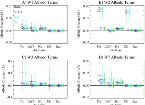
Figure 3 illustrates the same set of albedo sensitivity terms for four different cases. The mean and 1 standard deviation of pairs of adjacent drop numbers (seven pairs from eight values of drop number) is indicated by the error bar range and midpoint, and the median is shown as a diamond. The W2 case from Fig. 2b is illustrated in Fig. 3b (black line), where cloud coverage dominates the change in albedo. Some cases have mostly small differentials for the terms, and only some values ofNchave large differentials, so the median is often near zero but the average (dominated by 1–2 cases) is non-zero. The base case (black) is the basic case using the autoconversion scheme of Khairoutdinov and Kogan (2000), hereafter KK2000. KK2000 represent autoconversion from a fit to cloud-resolving model experiments as a function of the
cloud mass and an inverse function of drop number; the au-toconversion rate (Au) isAu=1350qc2.47Nc−1.79. This is also true for W1 (Fig. 3a), with lower sensitivity. However, the LWP andNcchanges are important in the W3 and W7 cases (Fig. 3c and d). These are weaker multiple updraft cases.
Also shown in Fig. 3 are three additional sets of experi-ments where the microphysics has been modified to limit the lifetime effects. This has been done by specifying a constant fixed drop number of 100 cm−3 to (a) the autoconversion scheme (Au), and (b) the sedimentation (Sed) or both (No-Lif). Different drop numbers ranging from 10 to 2000 cm−3 are used for all other processes in the microphysics. The No-Lif cases (dark blue in Fig. 3) are similar to the Au cases (green: autoconversion effects only) indicating that autocon-version is the dominant process for lifetime effects. In partic-ular, removing the lifetime effects by specifying the number concentration going into autoconversion removes the cloud coverage effects in the W2 case (Fig. 3b), and perhaps more significantly removes the LWP effects on albedo in all cases. This leaves only the drop number effects on albedo. Thus, for some cases with partial cloud cover (e.g., like the W2 case in Fig. 3b), lifetime effects are important for cloud cover changes, but in all cases the effect of autoconversion in drop number seems to impact LWP.
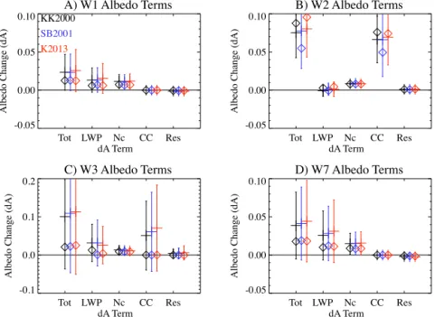
Recognizing that the representation of autoconversion is important, we explore two alternatives. Kogan (2013), hereafter K2013, use a similar representation as KK2000 and deriveAu=7.90×10¹⁰qc4.22Nc−3.01. Seifert and Beheng (2001), hereafter SB2001, derive expressions for autoconver-sion and accretion that include the rain water mixing ratio as a proxy for large cloud droplets to describe the broadening of the drop size distribution and reduce the efficiency of accre-tion in the early stage of the rain formaaccre-tion. We have imple-mented both of these parameterizations into the microphysics scheme.
Figure 4 shows the impact of the SB2001 scheme in the single updraft W1 case with a fixed drop number of 200 cm−3. Relative to KK2000 (black), the use of SB2001 (red) for autoconversion results in higher cloud mass (Fig. 4a), significantly less precipitation (Fig. 4b) and de-layed and smaller rain formation (Fig. 4c) and rain number concentration (Fig. 4d). Autoconversion (Fig. 4e) is delayed, but has a higher magnitude, and accretion is also delayed (Fig. 4f), but has a lower magnitude; the changes are sig-nificant. At lower number concentrations the differences are smaller, and they are larger at higher number concentrations (not shown).
A) W1 Albedo Terms
Tot LWP Nc CC Res dA Term
-0.05 0.00 0.05 0.10
A
lbe
do Cha
nge
(dA
)
Base NoLif
Sed Au
B) W2 Albedo Terms
Tot LWP Nc CC Res dA Term
-0.05 0.00 0.05 0.10
A
lbe
do Cha
nge
(dA
)
C) W3 Albedo Terms
Tot LWP Nc CC Res dA Term
-0.1 0.0 0.1 0.2
A
lbe
do Cha
nge
(dA
)
D) W7 Albedo Terms
Tot LWP Nc CC Res dA Term
-0.05 0.00 0.05 0.10
A
lbe
do Cha
nge
(dA
)
Figure 3.Albedo change by different sensitivity (dA) terms from different warm rain cases.(a)Warm 1,(b)warm 2,(c)warm 3 and(d)warm 7. Albedo terms in each panel correspond to the total (Tot) change and the portion due to liquid water path (LWP), number concentration (Nc), cloud coverage (CC) and a residual (Res); the standard case (Base) is in black. Also shown are the no lifetime effects case (dark blue)
and the two components of the lifetime effect: sedimentation (cyan) and autoconversion (green).
for SB2001 and K2013 (Fig. 5c), which is compensated for in-cloud cover changes. Autoconversion matters in the cases with multiple updrafts where cloud coverage is most sensi-tive (W2 and W3), and it matters more for the oscillating (W2) than decaying (W3) or weak (W7) updraft case. This is likely because with a limited temporal updraft the timing of precipitation matters.
4 Results: global sensitivity tests
Global sensitivity tests with CESM explore how different perturbations to cloud microphysics impact ACI. All tests are pairs of simulations with emissions of aerosols set to 2000 and 1850, except for the 2000–1750 and 1850–1750 cases, which use different emissions years to explore different mag-nitudes of emissions changes. The experiments described in Sect. 2.2 and Table 1 fall into several categories chosen to span key sensitivities in different microphysical processes. These are based on a number of previous studies that have identified these different processes as critical for the interac-tion of aerosols with clouds. These studies are highlighted below. The different processes include (1) aerosol activation (MG1) (Ghan et al., 2013; Carslaw et al., 2013), (2) precipita-tion (MG1.5, NoER: evaporaprecipita-tion of rain) (Wood et al., 2009; Jiang et al., 2010), (3) mixed phase (Berg0.1: vapor deposi-tion and Hoose: ice nucleadeposi-tion) (Hoose et al., 2010; Lawson and Gettelman, 2014), (4) autoconversion (lifetime effects and two other autoconversion schemes: K2013, SB2001)
(Wood et al., 2009; Gettelman et al., 2013), (5) coupling to other schemes (CLUBB) (Guo et al., 2011) and (6) natural emissions (Nat 0.5 and Nat2) (Carslaw et al., 2013). In par-ticular, the range of natural aerosol emissions is identical to the range in Carslaw et al. (2013).
The radiative changes between the pairs of simulations in each sensitivity experiment are indicated in Table 2. ACI use clean-sky CRE as discussed by Ghan et al. (2013). Dif-ferences in microphysical quantities are in Table 3. For Ta-ble 3 and the figures, simulated cloud-top liquid microphysi-cal values are estimated by taking the highest level (first from the top of the model going down) where cloud condensate is found. This is done at each point in the model and averaged over those points which are non-zero. The values and figures in the text come from these simulations. The net CRE for all the simulations (Table 3) is broadly similar, within about
±1 Wm−2, except for the MG2-CLUBB simulation, which has a different balance of CRE, drop number and effective radius (Table 3).
The radiative changes between the pairs of simulations in each sensitivity experiment are indicated in Fig. 6a. ACI are defined as the change in clean-sky cloud radiative effect (1CRE) between pairs of simulations with different aerosol emissions (Ghan et al., 2013). Directly using CRE yields similar quantitative (%) differences between simulations. ACI for 2000–1850 emissions are−1.57 Wm−2with MG1,
0 1000 2000 3000 4000 5000 Time (s)
0 1000 2000 3000
Z (m)
A) W1 Cloud Mass (g kg-1 )
KK2000 BLACK, SB2001 RED
0.2 0.6 1.0 1.4
B) W1 Surface Rain Rate (mm hr-1 )
KK2000 BLACK, SB2001 RED
0 1000 2000 3000 4000
Time (s) 0.0
0.5 1.0 1.5 2.0 2.5 3.0
Surface Rain Rate (mm hr
-1)
KK2000
SB2001
0 1000 2000 3000 4000 5000
Time (s) 0
1000 2000 3000
Z (m)
C) W1 Rain Mass (g kg-1)
KK2000 BLACK, SB2001 RED
0.05
0.05
0 1000 2000 3000 4000 5000
Time (s) 0
1000 2000 3000
Z (m)
D) W1 Rain Number Conc (kg-1)
KK2000 BLACK, SB2001 RED
1.50×10⁴ 4.50×10⁴ 7.50×10⁴
0 1000 2000 3000 4000 5000
Time (s) 0
1000 2000 3000
Z (m)
E) W1 Autoconversion Rate (kg kg-1 s-1
)
KK2000 BLACK, SB2001 RED
4.0×10⁻⁹
0 1000 2000 3000 4000 5000
Time (s) 0
1000 2000 3000
Z (m)
F) W1 Accretion Rate (kg kg-1 s-1)
KK2000 BLACK, SB2001 RED
Figure 4.Warm 1 (W1) single updraft case results with cloud drop number concentration of 200 cm−3for(a)cloud liquid mass (contour
interval 0.2 g kg−1),(b)surface precipitation rate,(c)warm rain mass (contour interval 0.05 g kg−1) and(d)rain number (contour interval 1.5×10⁴kg−1),(e)autoconversion rate (contour interval 4×10⁻⁹kg−1) and(f)accretion rate (contour interval 3×10⁻⁹kg−1) from MG2 with KK2000 (black) and SB2001 (red).
A) W1 Albedo Terms
Tot LWP Nc CC Res
dA Term -0.05
0.00 0.05 0.10
A
lbe
do Cha
nge
(dA
)
KK2000
SB2001 K2013
B) W2 Albedo Terms
Tot LWP Nc CC Res
dA Term -0.05
0.00 0.05 0.10
A
lbe
do Cha
nge
(dA
)
C) W3 Albedo Terms
Tot LWP Nc CC Res
dA Term -0.1
0.0 0.1 0.2
A
lbe
do Cha
nge
(dA
)
D) W7 Albedo Terms
Tot LWP Nc CC Res
dA Term -0.05
0.00 0.05 0.10
A
lbe
do Cha
nge
(dA
)
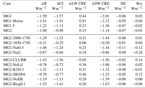
Table 2.Radiative impacts of ACI for the different sensitivity tests. Change in top-of-atmosphere (TOA) flux (1R), ACI as change in clean-sky cloud radiative effect (1CRE), and its long-wave (LW) and shortwave (SW) components following Ghan et al. (2013). Direct effects (DE) of aerosols as described in the text. Finally, a residual (Res=ACI + DE−1R).
Case 1R ACI 1LW CRE 1SW CRE DE Res
Wm−2 Wm−2 Wm−2 Wm−2 Wm−2 Wm−2
MG1 −1.59 −1.57 0.44 −2.01 −0.06 0.05
MG1-Hoose −1.61 −1.51 0.81 −2.32 −0.05 −0.04
MG1.5 −1.22 −1.13 0.23 −1.36 −0.07 −0.02
MG2 −1.08 −0.98 0.15 −1.14 −0.07 −0.03
MG2-2000-1750 −1.29 −1.23 0.21 −1.44 −0.08 0.01
MG2-1850-1750 −0.21 −0.25 0.06 −0.30 −0.01 0.04
MG2-Nat0.5 −1.46 −1.24 0.21 −1.44 −0.11 −0.12
MG2-Nat2 −0.87 −0.68 0.18 −0.86 0.09 −0.28
MG2-CLUBB −1.43 −1.56 −0.05 −1.50 −0.02 0.14
MG2-NoLif −0.78 −0.72 0.36 −1.08 −0.08 0.02
MG2-K2013 −1.21 −1.11 0.21 −1.32 −0.08 −0.01
MG2-SB2001 −0.70 −0.77 0.46 −1.23 −0.05 0.12
MG2-NoER −1.19 −1.11 0.29 −1.39 −0.08 0.00
MG2-Berg0.1 −1.53 −1.41 0.26 −1.67 −0.06 −0.06
occur. Northern Hemisphere midlatitudes are also where the largest changes to LWP (Fig. 6b) and cloud-top drop number concentration (1Nc, Fig. 6c) occur. Interestingly the changes to cloud-top drop effective radius (1Re, Fig. 6d) spread far-ther into high latitudes.
Most of the ACI are due to the shortwave (SW: solar) wavelengths: brighter clouds (Table 2). However, there is a significant component of positive ACI in the long-wave (LW: terrestrial) wavelengths. This is a result of two factors. First is the effect of aerosols on cirrus clouds, where more ice nu-clei are formed, and clouds become more opaque in the long wave than they become brighter in the shortwave (Gettelman et al., 2012). Second is a compensation effect between LW and SW for cirrus clouds due to movement of cirrus cloud fraction in the tropics. The second effect accounts for a good amount of the variance in the magnitude of the LW and SW between sensitivity tests: increases in LW CRE are compen-sated for by decreases in (increased magnitude of negative) SW CRE.
To understand how ACI change with cloud microphysics, we explore how the radiative effects of ACI are related to microphysical properties strongly related to radiative effects. Figure 7 illustrates some of the broad-scale patterns across the simulations, by relating the changes in cloud radiative effect (ACI=1CRE) to other properties of the simulations, namely, changes to LWP (in percent, Fig. 7a), changes to the cloud-top drop number concentration (Fig. 7b), changes to cloud-top effective radius (Fig. 7c) or changes in total (verti-cally integrated) cloud coverage or fraction (Fig. 7d). There is a strong correlation between 1LWP and ACI (Fig. 7a). The only simulations that differ from the correlation are those with CLUBB and the simulation without lifetime
ef-fects (NoLif). The CLUBB simulation has a very differ-ent coupling of large-scale condensation and cloud micro-physics, as described by Gettelman et al. (2015), where the microphysics is sub-stepped with the CLUBB condensation scheme six times in each time step. The NoLif simulation has basically no change in LWP, which is consistent with the off-line KiD tests with a similar formation. The ACI go from
−0.98 (MG2) to−0.72 Wm−2(NoLif) in Table 2. There is no correlation between the change in cloud-top drop number (Fig. 7b) or effective radius (Fig. 7c) and ACI. Changes in effective radius are negative, indicating smaller drops in the present with more aerosols than in the past (pre-industrial). There are small changes in total cloud cover that correlate slightly with ACI (Fig. 7d), but mostly because there are large changes (increases in cloud coverage) in three simu-lations with large ACI (CLUBB, MG1, MG1-Hoose).
The simulation without lifetime effects (NoLif) actually has the largest change (reduction) in averaged drop radius (Fig. 7c), despite no change in LWP (Fig. 7a) and small changes in ACI. Most simulations have an increase in cloud drop number of∼30 cm−3. This is an interesting result be-cause many models still prescribe the radiative effects of aerosols by linking aerosol mass to a change in cloud drop number or size; on the contrary, in CAM the clearest effects seem to be due to LWP, though ACI are non-zero even if
1LWP=0.
The following sub-sections detail each of the dimensions of changes to understand the magnitude of the effects. 4.1 Activation
A) Zonal Mean ACI
-60 -40 -20 0 20 40 60
Latitude -4 -3 -2 -1 0 1
ACI (W m
-2)
B) Zonal Mean ∆LWP
-60 -40 -20 0 20 40 60
Latitude -10 0 10 20 30 ∆ LWP (%)
C) Zonal Mean ∆Nc
-60 -40 -20 0 20 40 60
Latitude 0 20 40 60 80 100 ∆ Nc (cm-3) MG1 MG1-Hoose MG1.5 MG2 2000-1750 1850-1750 Nat0.5 Nat2 CLUBB NoLif K2013 SB2001 NoER Berg0.1
D) Zonal Mean ∆Re
-60 -40 -20 0 20 40 60
Latitude 0.5 0.0 -0.5 -1.0 -1.5 -2.0 ∆ Re (m-6)
Figure 6.Zonal mean(a)ACI (change in CRE, Wm−2),(b)percent change in LWP,(c)change in cloud-top drop number concentration (1Nc, cm−3) and(d)change in cloud-top effective radius (1Re, m−6) for different sensitivity tests noted with colors and different line
styles.
A) ACI v. ∆LWP
0.0 -0.5 -1.0 -1.5 -2.0
ACI (∆CRE) Wm-2
-2 0 2 4 6 8 10 ∆ L W P (%) MG1 MG1-Hoose MG1.5 MG2 2000-1750 1850-1750 Nat0.5 Nat2 CLUBB NoLif K2013 SB2001 NoER Berg0.1
B) ACI v. ∆Nc (Cld Top)
0.0 -0.5 -1.0 -1.5 -2.0
ACI (∆CRE) Wm-2
0 10 20 30 40 ∆ N c (c m -3 ) MG1 MG1-Hoose MG1.5 MG2 2000-1750 1850-1750 Nat0.5 Nat2 CLUBB NoLif K2013
SB2001 NoER Berg0.1
C) ACI v. ∆REL (Cld Top)
0.0 -0.5 -1.0 -1.5 -2.0
ACI (∆CRE) Wm-2 0.0 -0.2 -0.4 -0.6 -0.8 -1.0 ∆ RE L (m ic rons ) MG1 MG1-Hoose MG1.5 MG2 2000-1750 1850-1750 Nat0.5 Nat2 CLUBB NoLif K2013 SB2001 NoER Berg0.1
D) ACI v. ∆CTOT
0.0 -0.5 -1.0 -1.5 -2.0
ACI (∆CRE) Wm-2 -0.4 -0.2 0.0 0.2 0.4 0.6 ∆ CT O T (% ) MG1 MG1-Hoose MG1.5 MG2 2000-1750 1850-1750 Nat0.5 Nat2 CLUBB NoLif K2013 SB2001 NoER Berg0.1
Figure 7.ACI (change in CRE, Wm−2) vs.(a)percent change in LWP,(b)change in cloud-top drop number concentration (1Nc, cm−3),
(c)change in cloud-top effective radius (1REL, m−6or microns) and(d)change in total cloud coverage (CTOT, %) for different sensitivity
Table 3.Microphysical impact of different sensitivity tests. Mean CRE, change in LWP (%), mean LWP, change in cloud-top (CT) effective radius (REL), mean CT REL, change in CT drop number concentration (Nc) and mean CTNc.
Case CRE 1LWP LWP 1REL (CT) REL (CT) 1Nc (CT) Nc (CT)
Wm−2 % g m−2 m−6 m−6 cm−3 cm−3
MG1 −28.0 7.5 44.6 −0.4 9.5 22.5 89.0
MG1-Hoose −28.4 8.6 46.2 −0.5 9.5 22.2 88.6
MG1.5 −29.8 7.4 45.0 −0.6 8.8 29.4 110.6
MG2 −27.9 5.5 39.4 −0.6 9.0 28.9 107.2
MG2-2000-1750 −27.9 7.7 39.4 −0.8 9.0 35.0 107.2
MG2-1850-1750 −27.2 2.3 37.2 −0.2 9.6 6.1 78.3
MG2-Nat0.5 −27.6 6.5 38.2 −0.8 9.2 30.9 98.6
MG2-Nat2 −28.4 3.3 40.3 −0.5 8.6 26.0 119.8
MG2-CLUBB −25.6 4.8 40.1 −0.7 11.3 12.4 59.1
MG2-NoLif −28.7 −0.6 47.7 −0.9 9.4 27.5 107.9
MG2-K2013 −27.8 7.0 37.6 −0.6 8.9 28.6 107.4
MG2-SB2001 −28.3 3.6 44.6 −0.7 9.2 27.9 109.2
MG2-NoER −28.2 5.9 39.9 −0.6 9.0 28.6 106.9
MG2-Berg0.1 −28.7 7.2 44.0 −0.6 8.8 27.1 101.7
MG1 vs. MG1.5. This is a substantial reduction in ACI from
−1.57 to−1.13 Wm−2or 28 % (Table 2). The likely cause is that by activating the number first, other processes in the mi-crophysics act on the revised number, and this likely buffers the changes in the indirect effects (Stevens and Feingold, 2009). Note that there is basically no difference in the LWP change between MG1 and MG1.5 (Table 3). Effects are not simply linear, however, since MG1.5 with lower ACI has a larger1REL and1Nc.
4.2 Prognostic precipitation and rain evaporation
The major scientific changes between MG1.5 (MG1 with the activation change) and MG2 as described by Gettelman and Morrison (2015) are the addition of prognostic precipitation and the addition of evaporation of number when rain evap-orates. The latter change to evaporation of rain number ac-tually does seem to make a difference: a reduction in ACI (Table 2) due to a reduction in1LWP (Table 3). The total re-duction between MG1.5 and MG2 is−1.13 to−0.98 Wm−2, or about 14 %. This occurs through reductions in the1LWP (Table 3), especially between 10 and 60◦N latitude (Fig. 6b).
4.3 Mixed phase clouds
Two different sets of experiments were conducted to look at the impact of altering mixed phase clouds. The changes in MG1-Hoose make the simulations sensitive to anthropogenic aerosols in the mixed phase regime where they were not be-fore. This causes increases in the magnitude of the LW and SW components of ACI (Table 2), but a small change in the net ACI (−4 %). The sensitivity of LWP goes up (1LWP: Table 3). This experiment has the largest LW ACI, which is expected since it adds ACI in the mixed phase cloud regime
between 0 and−20◦C, which will have a significant effect
on the LW radiation.
The second experiment used the MG2 configuration to reduce the efficiency of the vapor deposition onto ice (Bergeron–Findeisen process) by a factor of 10. This sim-ulates inhomogeneity in cloud liquid and ice (or effectively inhomogeneity for in-cloud supersaturation or vertical ve-locity) that does not effectively mix liquid and ice. Korolev (2008) noted uncertainties of at least a factor of 2 in vapor deposition rates based on small-scale cloud dynamics, and Lawson and Gettelman (2014) found better agreement with Antarctic mixed phase clouds when vapor deposition was re-duced by a factor of 100. We picked a value between these limits for a sensitivity test. The reduction of vapor deposition increases the mean LWP and slightly decreases1LWP (Ta-ble 3). The stronger long-wave and shortwave components with more liquid likely lead to an increased magnitude in ACI (Table 2) of +45 %, but the exact mechanism is unclear.
4.4 Autoconversion and lifetime effects
As in Sect. 3, we can also explore the sensitivity of the micro-physics to autoconversion scheme. Gettelman et al. (2013) noted that the description of autoconversion and accretion matters for ACI, consistent with a series of previous studies (Menon et al., 2002; Rotstayn and Liu, 2005; Penner et al., 2006; Wang et al., 2012). One of the reasons for lower ACI in MG2 is due to the reduction of the ratio of autoconversion to accretion (more accretion and less autoconversion) with prognostic rain in MG2 (Gettelman et al., 2015).
A) 2000-1850
∆
TOA MG2
-12.5 -10.0 -7.50 -5.00 -2.50 2.500 5.000 7.500 10.00 12.50
Wm-2
B) 2000-1850
∆
TOA NoLif
Figure 8.ACI as the total change in the top-of-atmosphere clean-sky cloud radiative effect (CRE) between simulations with 2000 and 1850 aerosol emissions for(a)base (MG2) and(b)no lifetime effect (NoLif) cases.
consistent with an increase in1LWP (Table 3). Conversely, the SB2001 scheme, with a smaller 1LWP, reduces ACI from −0.98 to−0.77 Wm−2, or 22 %, and the NoLif sim-ulation reduces ACI to−0.72 Wm−2(nearly−30 %) largely through more compensation between LW and SW effects; i.e., larger LW effects, indicating clouds with cold cloud tops may have higher LW emissivity. This indicates that the lifetime effects themselves may approach one-third of ACI (the total change in radiative flux changes from −1.04 in MG2 to−0.78 in the NoLif simulation, a reduction of 33 %). The lifetime effects are not that sensitive to the drop num-ber threshold chosen. Results of a NoLif simulation with 300 cm−3rather than 100 cm−3 for liquid drops yield sim-ilar results for1R or ACI.
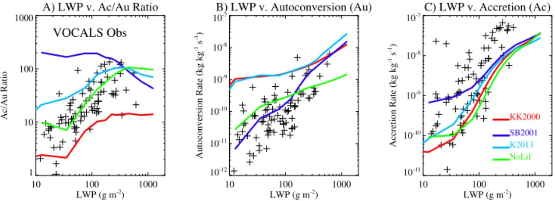
The regional pattern of ACI, based on the total change in top-of-atmosphere fluxes, is illustrated in Fig. 8 for (a) the base MG2 case and (b) the NoLif case. The average lo-cal standard deviation of annual TOA flux is about 3 Wm−2, so Fig. 8 shows regions with differences larger than 1 stan-dard deviation. ACI effects are mostly in the Northern Hemi-sphere, and mostly over the oceans. There are some tropical effects in Southeast Asia and off the equatorial eastern Pa-cific, the latter due to anthropogenic emissions over the Ama-zon. The removal of lifetime effects in Fig. 8b indicates they are strong over the Northern Hemisphere midlatitude storm tracks, especially in the North Pacific. Lifetime effects also are strong in the equatorial eastern Pacific. Lifetime effects do not seem to impact the stratocumulus region off the coast of California, which has strong ACI without lifetime effects. The effect of autoconversion and accretion is illustrated in Fig. 9. Figure 9 shows autoconversion and accretion rates and their ratio as a function of LWP. The figure compares re-sults to estimates based on observations from the VOCALS campaign in the southeastern Pacific (see the corrigendum to Gettelman et al. (2013) for more details). Note that the rates are estimated from using observations to approximate the re-sults of the stochastic collection equation, and may not be exactly comparable to the model simulations. The slope of the curves with LWP is probably the most relevant compari-son. The figure represents 60◦S–60◦N averages for all liquid
clouds treated by the stratiform cloud scheme, so it does not include convective clouds. A similar figure for just the
south-eastern Pacific region yields similar results, but not as good statistics.
Accretion rates (Ac) are well represented in MG2 with the KK2000 autoconversion (Fig. 9c), but autoconversion rates (Au) at low LWP are very large (Fig. 9b), leading to a low Ac/Au ratio (Fig. 9). With the SB2001 scheme, accretion is high at low LWP, and autoconversion is 2 orders of mag-nitude lower. Autoconversion in particular is much closer to estimates from VOCALS (Terai et al., 2012). The result is a higher Ac/Au ratio, which may be too high at low LWP. The K2013 scheme (cyan in Fig. 9) yields similar results to KK2000: autoconversion is almost the same, and accretion is a little bit higher. The no lifetime simulation (green in Fig. 9) has accretion rates similar to KK2000, but lower version rates due to fixing the drop number in the autocon-version scheme. The no lifetime simulation has perhaps the closest representation to the Ac/Au ratio (Fig. 9a).
4.5 Coupling to other schemes
We can also examine the effect of coupling of the micro-physics to other cloud schemes in the model. The CLUBB simulation uses a different unified higher-order closure scheme to replace the CAM large-scale condensation, shal-low convection and boundary layer scheme, as described by Bogenschutz et al. (2013). It uses MG2 with a different sub-stepping strategy of 5 min time steps, called six times per model time step.
Notably, CLUBB provides a unified condensation scheme for the boundary layer, stratiform and shallow convection regimes, so that ACI are included in shallow cumulus regimes in this formulation. This results in a substantial in-crease in ACI from−0.98 to−1.56 Wm−2(just over 50 %). The change in LWP (1LWP) is moderate (Fig. 6b), and less than would be expected based on the ACI (Fig. 7a). CLUBB has a lower change in cloud-top drop number (Figs. 6c and 7b), but a large increase in cloud coverage (Fig. 7d), which likely is contributing to ACI. The increase appears to be occurring in the sub-tropics of the Northern and South-ern hemispheres (Fig. 6a) mostly from 20 to 40◦N over the
A) LWP v. Ac/Au Ratio
10 100 1000
LWP (g m-2)
1 10 100 1000
Ac/Au Ratio
VOCALS Obs
B) LWP v. Autoconversion (Au)
10 100 1000
LWP (g m-2)
10-12
10-11
10-10
10-9
10-8
10-7
Autoconversion Rate (kg kg
-1 s -1)
C) LWP v. Accretion (Ac)
10 100 1000
LWP (g m-2)
10-11
10-10
10-9
10-8
10-7
Accretion Rate (kg kg
-1 s -1)
KK2000
SB2001
K2013
NoLif
Figure 9.60◦S to 60◦N latitude(a)ratio of accretion to autoconversion,(b)autoconversion rate and(c)accretion rate using KK2000 (red), SB2001 (dark blue), K2013 (cyan) autoconversion and the no lifetime (NoLif) simulation (green). Estimates derived from observations from the VOCALS experiment shown as black crosses (see text for details).
exploration of the impacts of this change is warranted but is beyond the scope of this work. Also notable is that CLUBB simulations have a decrease in the positive LW ACI. This occurs in the tropics, and may be related to changes in trans-port of water vapor into the upper troposphere, reducing high cloudiness and any positive ACI associated with high (cirrus) clouds. These changes may also be due to differences in how CLUBB treats aerosols and aerosol scavenging in these sim-ulations: it appears that the change in aerosol optical depth (AOD) is larger in CLUBB than in other simulations, perhaps due to different treatment of aerosol scavenging and transport in CLUBB. Thus, a very different physical parameterization suite with the same microphysical process rates can lead to very different ACI.
4.6 Background emissions
Finally, we explore the impact of background emissions on ACI. For these experiments no changes to the model are made. The experiments here all use the MG2 code. The only changes are to the emissions files. First, we just ex-plore what happens with different baselines: a larger period (2000–1750) or a smaller period (1850–1750) than the ba-sic 2000–1850 (MG2). As noted, for 1750 emissions, we re-move all human sources from the 1850 emissions. So this is really a no anthropogenic emissions case. Figure 7a illus-trates that the 2000–1750, MG2 and 1850–1750 changes are fairly linear, with LWP changing about 1 % per−0.1 Wm−2 change in ACI. The changes are also somewhat linear for changes to cloud-top drop number (Fig. 7b) and effective radius (Fig. 7c). Larger changes occur with higher emis-sions differences. This is not true for cloud coverage changes however (Fig. 7d), where MG2 (2000–1850) and 2000–1750 have about the same decreases in cloud coverage, while there is no change for 1850–1750.
Carslaw et al. (2013) found±20 % effects on ACI from the assumed level of background emissions. Similar to Carslaw et al. (2013) we conducted experiments by halving (Nat0.5)
or doubling (Nat2) the natural emissions of aerosols from dust, volcanoes, ocean dimethylsulfide (DMS) and natural organic carbon (terpenes and other biological aerosols). This was done for both pre-industrial and present emissions. Halv-ing natural emissions makes the model more sensitive to an-thropogenic aerosols (−1.13 to−1.24 Wm−2ACI in Table 2, a 27 % increase), whereas doubling emissions decreases the sensitivity significantly (−0.98 to−0.68 Wm−2ACI in Ta-ble 2, a 30 % decrease). The total change in TOA flux (dR) ranges from−1.46 (+34 %) to−0.87 Wm−2(−17 %) in Ta-ble 2. There is little change in LW ACI. Thus we can con-clude that the background natural aerosols are important for determining the total ACI.
The variation in natural emissions alters present-day AOD. Global mean AOD for Nat2, baseline (Nat1) and Nat0.5 is 0.175, 0.137 and 0.117, respectively, with most of the differ-ence caused by the imposed change to the efficiency of dust production and the dust AOD of 0.042, 0.024 and 0.013, re-spectively, for natural emissions scaling of 2, 1 and 0.5. This highlights and confirms the need to better constrain back-ground aerosols identified by Carslaw et al. (2013).
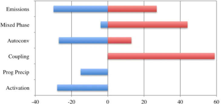
4.7 Summary of sensitivity tests
-40 -20 0 20 40 60 Activation
Prog Precip Coupling Autoconv Mixed Phase Emissions
Figure 10.Percent change in ACI for different dimensions of sen-sitivity tests as described in the text.
between accretion and autoconversion: with more accretion using prognostic rain.
Changes to the mixed phase of clouds, in particular a re-duction of the rate of vapor deposition (Berg0.1) to account for sub-grid inhomogeneity, result in an increase in the sen-sitivity of ACI to LWP. Reducing vapor deposition in the mixed phase increases the occurrence of liquid over ice. Liq-uid has a longer lifetime (and hence larger average shortwave radiative effect), and liquid clouds are more readily affected by sulfate aerosols than ice clouds are (only homogeneous freezing is affected by sulfate). The change to mixed phase ice nucleation (Hoose) has little impact on the net ACI, but a big impact on the LW. LW and SW effects for colder clouds tend to nearly cancel, with a slightly positive residual (simi-lar to the net cloud forcing for cold clouds), so the LW does not have a strong effect typically on the net ACI in the sen-sitivity tests, but it does show that changes to colder clouds that effect the LW may increase the gross magnitude of ACI. Coupling of the microphysics to different turbulence clo-sures and adding the treatment of ACI in shallow convection (CLUBB) alters ACI by over 50 % (Fig. 10). ACI in deep convection are still not treated, and this may also be impor-tant for ACI (Lohmann et al., 2008).
Changing activation to allow all processes to see re-vised number concentrations lowers ACI by 25 % (MG1 vs. MG1.5), likely due to buffering of the change to activation by other processes in the microphysics.
These microphysical effects are larger than aerosol pro-cesses or emissions uncertainties (the “A” in ACI). Natural (or background) emissions can alter the ACI significantly with the same cloud microphysics code, seen in the emis-sions bar in Fig. 10, with variability from −30 to +30 %, consistent with previous work (Carslaw et al., 2013), indi-cating±20 % sensitivity of ACI to similar perturbations of natural emissions. Carslaw et al. (2013) also noted ACI sen-sitivity of±10 % to aerosol processes, much smaller than the sensitivity to microphysical processes noted here.
5 Discussion/conclusions
Results of idealized and global model tests of a cloud mi-crophysics scheme indicate strong sensitivity of ACI, the ra-diative response of clouds to aerosol perturbations, to cloud microphysics. Idealized experiments illustrate the different dimensions of aerosol–cloud interactions, and how differ-ent cloud regimes may be affected in differdiffer-ent ways by ide-alized aerosol perturbations. The ideide-alized tests show that the representation of the autoconversion process is critical for cloud microphysical response to different drop numbers. These tests are consistent with and help motivate global sen-sitivity tests.
The sensitivity of ACI to the cloud microphysics with MG2 is−30 to +55 %, larger than the effects of background emissions (−30 to +30 %). Better representations of cloud microphysical processes (the “C” in ACI) are critical for rep-resenting the total forcing from changes in aerosols. These effects are stronger than uncertainties in aerosol emissions or processes. These sensitivity tests are not exhaustive in any statistical sense but form a baseline based on expert judge-ment, including processes identified by previous work that have been found to be important. We also note that the rel-ative importance between these dimensions of microphysics and aerosols is important. A more significant perturbed pa-rameter ensemble, similar in spirit to Carslaw et al. (2013) but including cloud microphysical uncertainties, is currently being developed.
Uncertain lifetime effects are manifest in CESM through changes to LWP with changes in aerosols. Lifetime effects in CESM represent about one-third of the total ACI. The mixed phase and the shallow convective regimes are also important, indicating that aerosol effects in convective clouds should be considered. Autoconversion parameterizations in partic-ular seem to specify lifetime effects that are highly uncer-tain. Many global models still prescribe cloud drop number or size based on aerosol mass. This may be problematic as interactions with different microphysical processes are im-portant for the magnitude of ACI.
How general are these results across models? The model framework with MG2 is a typical two-moment bulk micro-physics scheme with a framework similar to other schemes. Many of the process rate formulations for autoconversion examined here (e.g., KK2000) are used by other schemes as well. The sensitivity to background aerosol emissions is very similar to that diagnosed by Carslaw et al. (2013). In addition, the sensitivity of the microphysical process rates to autoconversion and accretion that occurs with prognostic precipitation is qualitatively similar to Posselt and Lohmann (2008). However, adding aerosol effects in all convective clouds (deep and shallow) in a different GCM reduced the ACI (Lohmann et al., 2008).
are in the process of developing such a cross-model compar-ison. The overall conclusion is that getting better a represen-tation of ACI is critical for reducing uncertainty in anthro-pogenic climate forcing: cloud microphysical development needs to go hand in hand with better constraints on aerosol emissions to properly constrain ACI and total forcing.
Acknowledgements. Thanks to A. Seifert for comments, discussion and inspiration and to C.-C. Chen for discussions. Computing resources were provided by the Climate Simulation Laboratory at National Center for Atmospheric Research (NCAR) Computational and Information Systems Laboratory. NCAR is sponsored by the U.S. National Science Foundation (NSF). This work was partially conducted on a visit with support of the Max Planck Institute for Meteorology, Hamburg, Germany.
Edited by: C. Hoose
References
Abdul-Razzak, H. and Ghan, S. J.: A parameterization of aerosol activation 2. Multiple aerosol types, J. Geophys. Res., 105, 6837– 6844, 2000.
Abdul-Razzak, H. and Ghan, S. J.: A parameterization of aerosol ac-tivation 3. Sectional Representation, J. Geophys. Res., 107, AAC 1-1–AAC 1-2, doi:10.1029/2001JD000483, 2002.
Albrecht, B. A.: Aerosols, cloud microphysics and fractional cloudiness, Science, 245, 1227–1230, 1989.
Bogenschutz, P. A., Gettelman, A., Morrison, H., Larson, V. E., Craig, C., and Schanen, D. P.: Higher-order turbulence closure and its impact on Climate Simulation in the Community Atmo-sphere Model, J. Climate., 26, 9655–9676, doi:10.1175/JCLI-D-13-00075.1, 2013.
Boucher, O., Randall, D., Artaxo, P., Bretherton, C., Feingold, G., Forster, P., Kerminen, V.-M., Kondo, Y., Liao, H., Lohmann, U., Rasch, P., Satheesh, S. K., Sherwood, S., Stevens, B., and Zhang, X. Y.: Clouds and Aerosols, in: Climate Change 2013: The Phys-ical Science Basis. Contribution of Working Group I to the Fifth Assessment Report of the Intergovernmental Panel on Climate Change, edited by: Stocker, T. F., Qin, D., Plattner, G.-K., Tig-nor, M., Allen, S. K., Boschung, J., Nauels, A., Xia, Y., Bex, V., and Midgley, P. M., Cambridge Universtiy Press, 2013. Carslaw, K., Lee, L., Reddington, C., Pringle, K., Rap, A., Forster,
P., Mann, G., Spracklen, D., Woodhouse, M., Regayre, L., and others: Large contribution of natural aerosols to uncertainty in indirect forcing, Nature, 503, 67–71, doi:10.1038/nature12674, 2013.
Gettelman, A. and Morrison, H.: Advanced Two-Moment Bulk Microphysics for Global Models. Part I: Off-Line Tests and Comparison with Other Schemes, J. Climate, 28, 1268–1287, doi:10.1175/JCLI-D-14-00102.1, 2015.
Gettelman, A., Liu, X., Barahona, D., Lohmann, U., and Chen, C. C.: Climate Impacts of Ice Nucleation, J. Geophys. Res., 117, D20201, doi:10.1029/2012JD017950, 2012.
Gettelman, A., Morrison, H., Terai, C. R., and Wood, R.: Micro-physical process rates and global aerosol-cloud interactions,
At-mos. Chem. Phys., 13, 9855–9867, doi:10.5194/acp-13-9855-2013, 2013.
Gettelman, A., Morrison, H., Santos, S., Bogenschutz, P., and Caldwell, P. M.: Advanced Two-Moment Bulk Micro-physics for Global Models. Part II: Global Model Solutions and Aerosol–Cloud Interactions, J. Climate, 28, 1288–1307, doi:10.1175/JCLI-D-14-00103.1, 2015.
Ghan, S. J.: Technical Note: Estimating aerosol effects on cloud radiative forcing, Atmos. Chem. Phys., 13, 9971–9974, doi:10.5194/acp-13-9971-2013, 2013.
Ghan, S. J., Smith, S. J., Wang, M., Zhang, K., Pringle, K., Carslaw, K., Pierce, J., Bauer, S., and Adams, P.: A simple model of global aerosol indirect effects, J. Geophys. Res.-Atmos., 118, 6688– 6707, doi:10.1002/jgrd.50567, 2013.
Guo, H., Golaz, J.-C., and Donner, L. J.: Aerosol effects on stratocu-mulus water paths in a PDF-based parameterization, Geophys. Res. Lett., 38, L17808, doi:10.1029/2011GL048611, 2011. Hoose, C., Kristjansson, J. E., Chen, J. P., and Hazra, A.: A
classical-theory-based parameterization of heterogeneous ice nucleation by mineral dust, soot and biological particles in a global climate model, J. Atmos. Sci., 67, 2483–2503, doi:10.1175/2010JAS3425.1, 2010.
Jiang, H., Feingold, G., and Sorooshian, A.: Effect of Aerosol on the Susceptibility and Efficiency of Precipitation in Warm Trade Cumulus Clouds, J. Atmos. Sci., 67, 3526–3540, 2010. Khairoutdinov, M. F. and Kogan, Y.: A new cloud physics
param-eterization in a large-eddy simulation model of marine stratocu-mulus, Mon. Weather Rev., 128, 229–243, 2000.
Kiehl, J. T., Schneider, T. L., Rasch, P. J., and Barth, M. C.: Ra-diative forcing due to sulfate aerosols from simulations with the National Center for Atmospheric Research Community Climate Model, version 3, J. Geophys. Res., 105, 1441–1457, 2000. Kogan, Y.: A Cumulus Cloud Microphysics Parameterization
for Cloud-Resolving Models, J. Atmos. Sci., 70, 1423–1436, doi:10.1175/JAS-D-12-0183.1, 2013.
Korolev, A.: Limitations of the Wegener–Bergeron–Findeisen Mechanism in the Evolution of Mixed-Phase Clouds, J. Atmos. Sci., 64, 3372–3375, doi:10.1175/JAS4035.1, 2007.
Korolev, A. V.: Rates of phase transformations in mixed-phase clouds, Q. J. Roy. Meteorol. Soc., 134, 595–608, doi:10.1002/qj.230, 2008.
Lawson, R. P. and Gettelman, A.: Impact of Antarctic mixed-phase clouds on climate, P. Natl. Acad. Sci. USA, 111, 18156–18161, doi:10.1073/pnas.1418197111, 2014.
Liu, X., Penner, J. E., and Wang, M.: Inclusion of ice microphysics in the NCAR Community Atmosphere Model version 3 (CAM3), J. Climate, 20, 4526–4547, 2007.
Liu, X., Easter, R. C., Ghan, S. J., Zaveri, R., Rasch, P., Shi, X., Lamarque, J.-F., Gettelman, A., Morrison, H., Vitt, F., Conley, A., Park, S., Neale, R., Hannay, C., Ekman, A. M. L., Hess, P., Mahowald, N., Collins, W., Iacono, M. J., Bretherton, C. S., Flan-ner, M. G., and Mitchell, D.: Toward a minimal representation of aerosols in climate models: description and evaluation in the Community Atmosphere Model CAM5, Geosci. Model Dev., 5, 709–739, doi:10.5194/gmd-5-709-2012, 2012.
Lohmann, U., Spichtinger, P., Jess, S., Peter, T., and Smit, H.: Cir-rus cloud formation and ice supersaturated regions in a global climate model, Environ. Res. Lett., 3, 045022, http://stacks.iop. org/1748-9326/3/045022, 2008.
Menon, S., Genio, A. D. D., Koch, D., and Tselioudis, G.: GCM Simulations of the Aerosol Indirect Effect: Sensitivity to Cloud Parameterization and Aerosol Bur-den, J. Atmos. Sci., 59, 692–713, doi:10.1175/1520-0469(2002)059<0692:GSOTAI>2.0.CO;2, 2002.
Meyers, M. P., DeMott, P. J., and Cotton, W. R.: New Primary Ice-Nucleation Parameterizations in an Explicit Cloud Model, J. Appl. Meteorol., 31, 708–721, 1992.
Morrison, H. and Gettelman, A.: A new two-moment bulk strati-form cloud microphysics scheme in the NCAR Community At-mosphere Model (CAM3), Part I: Description and Numerical Tests, J. Climate, 21, 3642–3659, 2008.
Neale, R. B., Chen, C. C., Gettelman, A., Lauritzen, P. H., Park, S., Williamson, D. L., Conley, A. J., Garcia, R., Kinnison, D., Lamarque, J. F., Marsh, D., Mills, M., Smith, A. K., Tilmes, S., Vitt, F., Cameron-Smith, P., Collins, W. D., Iacono, M. J., Easter, R. C., Ghan, S. J., Liu, X., Rasch, P. J., and Taylor, M. A.: Description of the NCAR Community Atmosphere Model (CAM5.0), Tech. Rep. NCAR/TN-486+STR, National Center for Atmospheric Research, Boulder, CO, USA, 2010.
Penner, J. E., Quaas, J., Storelvmo, T., Takemura, T., Boucher, O., Guo, H., Kirkevåg, A., Kristjánsson, J. E., and Seland, Ø.: Model intercomparison of indirect aerosol effects, Atmos. Chem. Phys., 6, 3391–3405, doi:10.5194/acp-6-3391-2006, 2006.
Pincus, R. and Baker, M. B.: Effect of precipitation on the albedo susceptibility of clouds in the marine boundary layer, Nature, 372, 250–252, 1994.
Posselt, R. and Lohmann, U.: Introduction of prognostic rain in ECHAM5: design and single column model simulations, At-mos. Chem. Phys., 8, 2949–2963, doi:10.5194/acp-8-2949-2008, 2008.
Rosenfeld, D., Lohmann, U., Raga, G. B., O’Dowd, C. D., Kul-mala, M., Fuzzi, S., Reissell, A., and Andreae, M. O.: Flood or Drought: How do Aerosols Affect Precipitation, Science, 321, 1309–1313, 2008.
Rotstayn, L. D. and Liu, Y.: A smaller global estimate of the sec-ond indirect aerosol effect, Geophys. Res. Lett., 32, L05708, doi:10.1029/2004GL021922, 2005.
Seifert, A. and Beheng, K. D.: A double-moment parameterization for simulating autoconversion, accretion and selfcollection, At-mos. Res., 59–60, 265–281, 2001.
Shipway, B. J. and Hill, A. A.: Diagnosis of systematic differences between multiple parametrizations of warm rain microphysics using a kinematic framework, Q. J. Roy. Meteorol. Soc., 138, 2196–2211, doi:10.1002/qj.1913, 2012.
Stevens, B. and Feingold, G.: Untangling aerosol effects on clouds and precipitation in a buffered system, Nature, 461, 607–613, 2009.
Terai, C. R., Wood, R., Leon, D. C., and Zuidema, P.: Does pre-cipitation susceptibility vary with increasing cloud thickness in marine stratocumulus?, Atmos. Chem. Phys., 12, 4567–4583, doi:10.5194/acp-12-4567-2012, 2012.
Twomey, S.: The influence of pollution on the shortwave albedo of clouds, J. Atmos. Sci., 34, 1149–1152, 1977.
Twomey, S. and Squires, P.: The Influence of Cloud Nucleus Popu-lation on the Microstructure and Stability of Convective Clouds, Tellus, 9, 408–411, 1959.
Wang, M., Ghan, S., Liu, X., L’Ecuyer, T. S., Zhang, K., Morrison, H., M. Ovchinnikov, R. E., Marchand, R., Chand, D., Qian, Y., and Penner, J. E.: Constraining cloud lifetime effects of aerosols using A-Train Satellite observations, Geophys. Res. Lett., 39, L15709, doi:10.1029/2012GL052204, 2012.
Wood, R., Kubar, T. L., and Hartmann, D. L.: Understand-ing the Importantce of Microphysics and Macrophysics for Warm Rain in Marine Low Clouds. Part II: Heuristic Mod-els of Rain Formation, J. Atmos. Sci., 66, 2973–2990, doi:10.1175/2009JAS3072.1, 2009.
Zhang, Y., Stevens, B., and Ghil, M.: On the diurnal cycle and susceptibility to aerosol concentration in a stratocumulus-topped mixed layer, Q. J. Roy. Meteorol. Soc., 131, 1567–1583, doi:10.1256/qj.04.103, 2005.