Opinion dynamics with confirmation bias.

Armen E. Allahverdyan1*, Aram Galstyan2

1Department of Theoretical Physics, Yerevan Physics Institute, Yerevan, Armenia,2USC Information Sciences Institute, Marina del Rey, California, United States of America

Abstract

Background:Confirmation bias is the tendency to acquire or evaluate new information in a way that is consistent with one’s preexisting beliefs. It is omnipresent in psychology, economics, and even scientific practices. Prior theoretical research of this phenomenon has mainly focused on its economic implications possibly missing its potential connections with broader notions of cognitive science.

Methodology/Principal Findings:We formulate a (non-Bayesian) model for revising subjective probabilistic opinion of a confirmationally-biased agent in the light of a persuasive opinion. The revision rule ensures that the agent does not react to persuasion that is either far from his current opinion or coincides with it. We demonstrate that the model accounts for the basic phenomenology of the social judgment theory, and allows to study various phenomena such as cognitive dissonance and boomerang effect. The model also displays the order of presentation effect–when consecutively exposed to two opinions, the preference is given to the last opinion (recency) or the first opinion (primacy) –and relates recency to confirmation bias. Finally, we study the model in the case of repeated persuasion and analyze its convergence properties. Conclusions:The standard Bayesian approach to probabilistic opinion revision is inadequate for describing the observed phenomenology of persuasion process. The simple non-Bayesian model proposed here does agree with this phenomenology and is capable of reproducing a spectrum of effects observed in psychology: primacy-recency phenomenon, boomerang effect and cognitive dissonance. We point out several limitations of the model that should motivate its future development.

Citation:Allahverdyan AE, Galstyan A (2014) Opinion Dynamics with Confirmation Bias. PLoS ONE 9(7): e99557. doi:10.1371/journal.pone.0099557

Editor:Pablo Branas-Garza, Middlesex University London, United Kingdom

ReceivedDecember 8, 2013;AcceptedMay 15, 2014;PublishedJuly 9, 2014

Copyright:ß2014 Allahverdyan, Galstyan. This is an open-access article distributed under the terms of the Creative Commons Attribution License, which permits unrestricted use, distribution, and reproduction in any medium, provided the original author and source are credited.

Funding:This research was supported by DARPA grant No. W911NF-12-1-0034 and AFOSR MURI grant No. FA9550-10-1-0569. The funders had no role in study design, data collection and analysis, decision to publish, or preparation of the manuscript.

Competing Interests:The authors have declared that no competing interests exist. * Email: [email protected]

Introduction

Confirmation bias is the tendency to acquire or process new information in a way that confirms one’s preconceptions and avoids contradiction with prior beliefs [52]. Various manifestations of this bias have been reported in cognitive psychology [5,67], social psychology [24,54], politics [46] and (media) economics [31,51,57,73]. Recent evidence suggests that scientific practices too are susceptible to various forms of confirmation bias [12,38,43,44,52], even though the imperative of avoiding precisely this bias is frequently presented as one of the pillars of the scientific method.

Here we are interested in the opinion revision of an agent_P who is persuaded (or advised) by another agent _Q [10,13,52]. (Below we use the terms opinion and beliefinterchangeably.) We follow the known framework for representing uncertain opinions of both agents via the subjective probability theory [13]. Within this framework, the opinion of an agent about propositions (events) is described by probabilities that quantify his degree of confidence in the truth of these propositions [13]. As we argue in the next section, the standard Bayesian approach to opinion revision is inadequate for describing persuasion. Instead, here we study confirmationally-biased persuasion within the opinion combina-tion approach developed in statistics; see [21,30] for reviews.

We suggest a set of conditions that model cognitive aspects of confirmation bias. Essentially, those conditions formalize the

intuition that the agent _P does not change his opinion if the persuasion is either far away or identical with his existing opinion [15,60]. We then propose a simple opinion revision rule that satisfies those conditions and is consistent with the ordinary probability theory. The rule consists of two elementary operations: averagingthe initial opinion with the persuading opinion via linear combination, and then projectingit onto the initial opinion. The actual existence of these two operations has an experimental support [8,9,18,72,].

We demonstrate that the proposed revision rule is consistent with the social judgment theory [10], and reproduces the so called change-discrepancy relationship [10,35,40,45,69]. Furthermore, the well-studiedweighted averageapproach [9,27] for opinion revision is shown to be a particular case of our model.

The rest of this paper is organized as follows. In the next section we introduce the problem setup and provide a brief survey of relevant work, specifically focusing on inadequacy of the standard Bayesian approach to opinion revision under persuasion. In the third section we define our axioms and introduce the confirma-tionally biased opinion revision rule. The fourth section relates our setup to the social judgment theory. Next two sections describe how our model accounts for two basic phenomena of experimental social psychology: opinion change versus discrepancy and the order of presentation effect. The seventh section shows how our model formalizes features of cognitive dissonance, followed by analysis of opinion change under repeated persuasion. Then we study theboomerang effect–the agent changes his opinion not towards the persuasion, but against it– as a particular case of our approach. We summarize and conclude in the last section.

The Set-Up and Previous Research

Consider two agentsP and Q. They are given an uncertain quantity (random variable) _X with values k~1,:::,N, e.g. k~_ðrain,norain_Þ, if this is a weather forecast. _X constitutes the state of the world for P and Q. The opinions of the agents are quantified via probabilities

p~f gpk Nk~1andq~f gqk Nk~1, XN

k~1 pk~

XN

k~1

qk~1 ð1Þ

for_Pand_Qrespectively.

Let us now assume that P is persuaded (or advised) by Q. (Persuasion and advising are not completely equivalent [71]. However, in the context of our discussion it will be useful to employ both terms simultaneously stressing their commmon aspects.) Throughout this paper we assume that the state of the world does not change, and that the agents are aware of this fact. Hence,_Pis going to change his opinion only under influence of the opinion ofQ, and not due to any additional knowledge about

X(For more details on this point see [3,41] and the second section of File S1.)

The normative standard for opinion revision is related to the Bayesian approach. Below we discuss the main elements of the Bayesian approach, and outline certain limitations that motivates the non-Bayesian revision rule suggested in this work.

Within the Bayesian approach, the agent P treats his own probabilistic opinionp~_fpkgN_k~1as a prior, and the probabilistic opinion q~_fqkgNk~1 ofQ as an evidence [28,30,47]. Next, it is assumed that_P is endowed with conditional probability densities P(qDk), which statistically relate q to the world state k. Upon receiving the evidence fromQ, agentPmodifies his opinion from pktop(kDq)via the Bayes rule:

p(kDq)~_P(qDk)pk=

XN

l~1

P(qDl)pl: ð2Þ

One issue with the Bayesian approach is that the assumption on the existence and availability of P(qDk) may be too strong [13,25,30]. Another issue is that existing empirical evidence suggests that people do not behave according to the Bayesian approach [13,61], e.g. they demonstrate the order of presentation effect, which is generally absent within the Bayesian framework.

In the context of persuasion, the Bayesian approach (2) has two additional (and more serious) drawbacks. To explain the first drawback, let us make a generic assumption that there is a unique

index^kkfor whichP(qDk) is maximized as a function ofk(for a givenq):P(qD^kk)w_P(qDk)for^kk~6 k.

Now consider repeated application of (2), which corresponds to the usual practice of repeated persuasion under the same opinionq of _Q. The opinion of the agent then tends to be completely polarized, i.e. p_kk^?1 and pk?0 for k~6 ^kk. In the context of

persuasion or advising, we would rather expect that under repeated persuasion the opinion of_Pwill converge to that of_Q.

The second issue is that, according to (2), _P will change his opinion even if he has the same opinion as_Q:p = q. This feature may not be realistic: we do not expectPto change his opinion, if he is persuaded towards the same opinion he has already. This drawback of (2) was noted in [28]. (Ref. [28] offers a modification of the Bayesian approach that complies with this point, as shown in [28] on one particular example. However, that modification betrays the spirit of the normative Bayesianism, because it makes conditional probabilities depending on the prior probability.)

It is worthwhile to note that researchers have studied several aspects of confirmation bias by looking at certain deviations from the Bayes rule, e.g. when the conditional probability are available, but the agent does not apply the proper Bayes rule deviating from it in certain aspects [31,51,57,73]. One example of this is when the (functional) form of the conditional probability is changed depending on the evidence received or on the prior probabilities. Another example is when the agent does not employ the full available evidence and selects only the evidence that can potentially confirm his prior expectations [39,48,67]. More generally, one has to differentiate between two aspects of the confirmation bias that can be displayed either with respect to information acquiring, or information assimilation (or both) [52]. Our study will concentrate on information assimilation aspect; first, because this aspect is not studied sufficiently well, and second, because because it seems to be more directly linked to cognitive limitations [52]. We also stress that we focus on the belief revision, and not on actions an agent might perform based on those beliefs.

Opinion Revision Rule

We propose the following conditions that the opinion revision rule should satisfy.

1.The revised opinion~ppkofP is represented as

~

p

pk~F½pk,qk=

XN

l~1F½pl,ql, ð3Þ

where F½x1,x2 is defined over x1[_½0,?_{) and x2}[_½0,?_{). We} enlarged the natural rangex1[_½0,1andx2[_½0,1, since below we plan to consider probabilities that are not necessarily normalized to 1. There are at least two reasons for doing so: First, experimental studies of opinion elicitation and revision use more general normalizations [8,9]. For example, if the probability is elicited in percents, the overall normalization is 100. Second, and more importantly, the axioms defining subjective (or logical) probabilities leave the overall normalization as a free parameter [22].

We require that F½x1,x2 is continuous for x1[_½0,?_{) and} x2[_½0,?₎and infinitely differentiable forx1[(0,?₎andx2[(0,?₎. Such (or similar) conditions are needed for features that are established for certain limiting values of the arguments ofF(cf. (5, 6)) to hold approximately whenever the arguments are close to those limiting values.Fcan also depend on model parameters, as seen below.

is local: assume that N§₃ and only the probability q1 is

communicated by _Q to _P. This suffices for _P to revise his probability fromp1to~pp1, and then adjust other probabilities via

renormalization:

~

p

p1~F½p1,q1=(F½p1,q1z1{p1),

e pk

pk~pk=ðF p1½ ,q1:z1{p1Þk§2: ð4Þ

Eq. (3) can be considered as a succession of such local processes. 2.Ifpk~0for somek, then~ppk~0:

F½0,y~0: ð5Þ

The rationale of this condition is that if_Psets the probability of a certain event strictly to zero, then he sees logical (or factual) reasons for prohibiting the occurrence of this event. Hence_P is not going to change this zero probability under persuasion.

3.Ifpkqk~0for allk, thenp~pk~pk:Pcannot be persuaded by Qif their opinions have no overlap.

4.If_Q’s and_P’s opinions are identical, then the latter will not

change his opinion: fpkgN

k~1~fqkg

N

k~1 (for all k) leads to

f~ppkgNk~1~fpkg

N

k~1. This can be written as

F½x,x~x: _ð6Þ

Conditions3 and 4 are motivated by experimental results in social psychology, which state that people are not persuaded by opinions that are either very far, or very close to their initial opinion [10,17,69].

(Recall that we do not allow the uncertain quantity_Xto change during the persuasion or advising. If such a change is allowed,4 may not be natural as the following example shows. Assume thatP

holds a probabilistic opinion(0:1,0:9)on a binary_X. Let_Plearns that_Xchanged, but he does not know in which specific way it did. Now _P meets _Qwho has the same opinion(0:1,0:9). Provided thatQdoes not echo the opinion ofP, the agentPshould perhaps change his opinion by decreasing the first probability (0.1) towards a smaller value, because it is likely that _X changed in that direction.)

5.Fis a homogeneous function of order one:

F_½cx,cy~cF x_½ ,yforc§0: _ð7_Þ

The rationale for this condition comes from the fact that (depending on the experimental situation) the subjective proba-bility may be expressed not in normalization one (i.e. not with

XN

k~1pk~

XN

k~1qk~1), but with a different overall normal-ization (e.g. XN_k~1pk~

XN

k~1qk~c) [8,9,22]; cf. 1. In this light, (7) simply states that any choice of the overall normalization is consistent with the sought rule provided that it is the same forP

and_Q. Any rescaling of the overall normalization by the factorc

will rescale the non-normalized probability by the same factorc; cf. (7).

6.Now we assume that the opinion assimilation by_Pconsists of two sub-processes. Both are related to heuristics of human judgement.

6.1 _P combines his opinion linearly with the opinion of _Q [8,9,18,29,30]:

^

p

pk~Epkz(1{E)qk, 0ƒEƒ1, ð8Þ

whereEis a weight. Several mathematical interpretations of the weightEwere given in statistics, where (8) emerged as one of the basic rules of probabilistic opinion combination [16,29]; see section I of File S1. One interpretation suggested by this approach is that E and 1{E are the probabilities–from the subjective viewpoint of_P–for, respectively,pandqto be the true description of states of the world [29]: it is not known to_Pwhich one of these probabilities (por q) conveys a more accurate reflection of the world state. Then_f^ppkgNk~1is just the marginal probability for the states of the world. There is also an alternative (normative) way of deriving (8) from maximization of an average utility that under certain natural assumptions can be shown to be the (negated) average information loss [16]; see section I of File S1 for more details.

Several qualitative factors contribute to the subjective assess-ment of E. For instance, one interpretation is to relate E to credibility ofQ(as perceived by P): more credibleQleads to a larger1{E[18]. Several other factors might affectE: egocentric attitude ofPthat tends to discount opinions, simply because they do not belong to him; or the fact thatP has access to internal reasons for choosing his opinion, while he is not aware of the internal reasons ofQetc[18]. Taking into account various factors that contribute to the interpretation ofE, we will treat it as a free model parameter.

6.2Note that (8) does not satisfy conditions2and3above. We turn to the last ingredient of the sought rule, which, in particular, should achieve consistency with conditions2and3.

Toward this goal, we assume that _P projects the linearly combined opinion^pp(see (8)) onto his original opinionp. Owing to (3), we write this transformation as

~

p

pk~w½pk,^ppk=

XN

l~1w½pl,^ppl, ð9Þ

where the functionwis to be determined.

The above projection operation relates to trimming [18,72], a human cognitive heuristics, wherePtends to neglect those aspects of Q’s opinion that deviate from a certain reference. In the simplest case this reference will be the existing opinion of_P.

To make the projection process (more) objective, we shall assume that it commutes with the probabilistic revision: whenever

p’_k~_PNckpk

l~1clpl ,ppbkk’~

c_kppbkk

PN l~1clppbll

, 1ƒkƒN, ð10Þ

wherec_k~Pr(:::Dk)w0are certain conditional probabilities,~ppis revised via the same rule (10):

~

p

p’_k:_Pw½p’k,^pp’k

N

l~1w½p’l,^pp’l

~_Pckw½pk,^ppk

N

l~1clw½pl,^ppl

: ð11Þ

This feature means that the projection is consistent with probability theory: it does not matter whether (3) is applied before or after (10).

w½pk, k~pmk

1{m

k , 0vmƒ1 ð12Þ

wheremquantifies the projection strength: form~1the projection is so strong that P does not change his opinion at all (conservatism), while for m?0, _P fully accepts ^pp(provided that pkw0for allk). (The above commutativity is formally valid also for mƒ0 ormw1, but both these cases are in conflict with (5).) In particular, E?0and m?0is a limiting case of a fully credulous agent that blindly follows persuasion provided that all his probabilities are non-zero. (For a sufficiently smallm, a smallpk is less effective in decreasing the final probability~ppk; see (12). This

is becausepm_k~_emlnpktends to zero for a fixedmandpk?0, while

it tends to one for a fixedpkandm?0. This interpaly between pk?0 and m?0is not unnatural, since the initial opinion of a

credulous agent is expected to be less relevant. The case of credulous agent is of an intrinsic interest and it does warrant further studies. However, since our main focus is confirmation bias, below we setm~1=2and analyze the opinion dynamics for varyingE.)

The final opinion revision rule reads from (12, 8, 9):

~

p pk~

ffiffiffiffiffiffiffiffiffiffiffiffiffiffiffiffiffiffiffiffiffiffiffiffiffiffiffiffiffiffiffiffiffiffiffiffi pk½Epkz(1{E)qk

p PN

l~1

ffiffiffiffiffiffiffiffiffiffiffiffiffiffiffiffiffiffiffiffiffiffiffiffiffiffiffiffiffiffiffiffiffi pl½Eplz(1{E)ql

p , 0ƒEƒ1: _ð13_Þ

It is seen to satisfy conditions1–5.

(Note that the analogue of (11),p’_k!_{ckpk, q}’_k!_{ckqk does not} leave invariant the linear function (8). First averaging, Epkz(1{E)qk and then applyingp’k!ckpk, q’k!ckqk is

equiva-lent to first applying the latter rules and then averaging with a different weight E’. This is natural: once E can be (in principle) interpreted as a probability it should also change under probabilistic revision process.)

The two processes were applied above in the specific order: first averaging (8), and then projection (9). We do not have any strong objective justifications for this order, although certain experiments on advising indicate on the order that led to (13) [72]. Thus, it is not excluded that the two sub-processes can be applied in the reverse order: first projection and then averaging. Then instead of (13) we get (3) with:

F p½ k,qk;E,m~Epkzð1{EÞpmkq

1{m

k , 0vmv1: ð14Þ

Our analysis indicates that both revision rules (13) and (14) (taken withm~1=2) produce qualitatively similar results. Hence, we focus on (13) for the remainder of this paper.

Returning to (1), we note that k = x can be a continuous variable, if (for example) the forecast concerns the chance of having rain or the amount of rain. Then the respective probability densities are:

p x_{ð Þ}andq x_{ð Þ}, ð

dx p x_{ð Þ}~ ð

dx q x_{ð Þ}~1: _ð15_Þ

Since the revision rule (13) is continuous and differentiable (in the sense defined after (3)), it supports a smooth transition between discrete probabilities and continuous and differentiable probability densities. In particular, (13) can be written directly for densities: for pk^p(xk)dxwe obtain from (13)

~

p p(x)~

ffiffiffiffiffiffiffiffiffiffiffiffiffiffiffiffiffiffiffiffiffiffiffiffiffiffiffiffiffiffiffiffiffiffiffiffiffiffiffiffiffiffiffiffiffiffiffiffiffiffi p(x)_½Ep(x)z(1{E)q(x) p

Ð

dx’pffiffiffiffiffiffiffiffiffiffiffiffiffiffiffiffiffiffiffiffiffiffiffiffiffiffiffiffiffiffiffiffiffiffiffiffiffiffiffiffiffiffiffiffiffiffiffiffiffiffiffiffiffiffi_p(x’_)½Ep(x’₎z(1{E)q(x’₎: ð16Þ

Social Judgment Theory and Gaussian Opinions

Opinion latitudes

Here we discuss our model in the context of the social judgment theory [59,10], and consider several basic scenarios of opinion change under the rule (16).

According to the social judgment theory, an agent who is exposed to persuasion perceives and evaluates the presented information by comparing it with his existing attitudes (opinions). The theory further postulates that an attitude is composed of three zones, or latitudes:acceptance, non-commitment and rejection [10,59]. The opinion that is most acceptable toP, or theanchor, is located at the center of the latitude of acceptance. The theory states that persuasion does not change the opinion much, if the persuasive message is either very close to the anchor or falls within the latitude of rejection [10,59]. The social judgment theory is popular, but its quantitative modeling has been rather scarce. In particular, to the best of our knowledge, there has been no attempt to develop a consistent probabilistic framework for the theory. (The literature on the social judgment theory offers some formal mathematical expressions that could be fitted to experimental data [45]. There is also a more quantitative theory [34] whose content is briefly reminded in section III of File S1.)

Let us assume thatk = xis a continuous variable (cf. (15)) and thatp(x) andq(x) are Gaussian with meanml and dispersion vl (l~P,Q):

p(x)~e

{(x {m_P)2

2v_P

ffiffiffiffiffiffiffiffiffiffi 2pvP

p , q(x)~e

{(x{mQ)2

2v_Q

ffiffiffiffiffiffiffiffiffiffiffi 2pvQ

p : ð17Þ

Effectively, Gaussian probabilistic opinions are produced in experiments, when the subjects are asked to generate an opinion with&95% confidence in a certain interval [18]. Now we can identify the anchor with the most probable opinionml, whilev{1 l quantifies the opinion uncertainty.

The latitude of acceptance amounts to opinions not far from the anchor, while the latitude of rejection contains close-to-zero probability events, sinceP does not change his opinion on them; recall point2from the previous section. One can also identify the three latitudes with appropriately chosen zones in the distribution. For instance, it is plausible to define the latitudes of acceptance and rejection by, respectively, the following formulas of the3srule known in statistics

x[½mP{2pffiffiffiffiffivP, mlz2pffiffiffiffiffivP, ð18Þ

x[({?_,mP{3pffiffiffiffiffivP|½mPz3pffiffiffiffiffivP,?), ð19Þ

where the latitude of non-commitment contains whatever is left out from (18, 19). Recall that the latitudes of acceptance, non-commitment and rejection carry (respectively) 95.4, 4.3 and 0.3% of probability.

While the definitions (18, 19) are to some extent arbitrary, they work well with the rule (16), e.g. if the opinions of_Pand_Qoverlap only within their rejection latitudes, then neither of them can effectively change the opinion of another. Also, _P is persuaded most strongly, if the anchor of the persuasion falls into the non-commitment latitude of _P. This is seen below when studying change-discrepancy relations.

Weighted average of anchors

Next, we demonstrate that the main quantitative theory of persuasion and opinion change–the weighted average approach [9,27] –is a particular case of our model. We assume that the opinionsp(x) andq(x) are given as

p(x)~_f(x{_{mP), p(x)}~_g(x{_{mQ), ð20Þ}

f’₍₀₎:_df=dxDx~0~g’(0)~0,

f’’₍₀₎v0, g’’₍₀₎v0, ð21Þ

where bothf(x) andg(x) have a unique maximum atx = 0. Hence p(x) (resp. q(x)) has a single anchor (maximally probable opinion) mP (resp.mQ); see (17) for concrete examples.

IfDmP{mQD is sufficiently small,~pp(x) given by (20, 16) has a single anchor which is shifted towards that ofq(x); see Fig. 1(a). We now look for the maximumm_e

P

P of~pp(x)by using (20) in (16). We neglect factors of order _O½(mP{mQ)2=vP and O½(mP{mQ)2=vQand deduce:

m_e P

P~(1{aQ)mPzaQmQ, ð22Þ

a_Q:

(1{E)Dg’’(0)D g(0)

(1{E)Dg’’(0)D g(0) z

Df’’(0)D f(0) 2E

f(0) g(0)z1{E

: _ð23Þ

Eq. (22) is the main postulate of the weighted average approach; see [9,27] for reviews. Herea_Qand1{a_Qare the weights of_Q and of_P, respectively. For the Gaussian case (17), we have

aQ~ 1zy 1z2E ffiffiffi y

p

1{E

{1

, y:vQ

v_P: ð24Þ

Furthermore, we have

LaQ

Ly

~{a2_Q 1z3E ffiffiffi y

p

1{E

,LaQ LE

~{2y 3=2_a2

Q 1{E

ð Þ , ð25Þ

Thus,a_Q’s dependence on the involved parameters is intuitively correct: it increases with the confidence1=v_Qof_Q, and decreases with the confidence1=v_Pof_P. Note also thata_Qdecreases withE. Now letp(x) andq(x) (and hence~pp(x)) have the same maximum mP~mQ, butvP&vQ; see (17). Expanding (16, 17) overvP{vQ and keeping the first-order term only we get

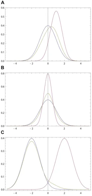
Figure 1. Opinions described via Gaussian densities (17). The initial opinion ofP is described by Gaussian probability densityp(x) (blue curve) centered at zero; see (17). The opinion ofQamounts to Gaussian probability densityq(x) (purple curve) centered at a positive value. For all three figures continuous density f(x) (f~p,q,~pp) were approximated by 100 pointsff(xk)g100

k~1,xkz1{xk~0:1. The resulting

opinion~pp(x)of P is given by (16) withE~0:5(olive curve). (a) The opinion ofPmoves towards that ofQ;m_P~0,s_P~1,m_Q~1,s_Q~0:5. (b) The maximally probable opinion ofPis reinforced;mP~0,s_P~1,

m_Q~0,s_Q~0:25. (c) The change of the opinion ofPis relatively small provided that the Gaussian densities overlap only in the region of non-commitment; cf. (18), (19). Whenever the densities overlap only within the rejection range the difference betweenp(x) and~pp(x)is not visible by eyes. For example, ifp(x) andq(x) are Gaussian with, respectively,

m_P~{3, m_Q~3, v_P~v_Q~1, the Hellinger distance (see (30) for definition)h½p,q~0:99 is close to maximally far, while the opinion change is small:h½p,~pp~3:48|10{2_.

v_e P P~

1{E 2 vQz

1zE

2 vP, ð26Þ

wherev_e P

Pis the dispersion of (non-Gaussian)~pp(x). Eq. (26) implies

(v_e P

P{vP)(vQ{vP)~ 1{E

2 (vQ{vP) 2_§0,

ð27_Þ

i.e. if 1=vQw1=vP (resp. 1=vQv1=vP), the final opinion of P becomes more (resp. less) narrow than his initial opinion. Fig. 1(b) shows that(v_e

P

P{vP)(vQ{vP)§0holds more generally.

Thus, the weighted average approach is a particular case of our model, where the agent _P is persuaded by a slightly different opinion. Note also that our model suggests a parameter structure of the weighted average approach.

Opinions and bump-densities

Gaussian densities (with three latitudes) do correspond to the phenomenology of social psychology. However, in certain scenarios one might need other forms of densities, e.g., when the probability is strictly zero outside of a finite support. Such opinions can be represented by bump-functions

X x_ð ;b_Þ~ _{ð Þ}bexp b x2{₁

forDxDv1 _ð28_Þ

~_{0 forx}ƒ{_{1 and x}§1:

where bw0 is a parameter, _N(b) is the normalization and the support of the bump function was chosen to be _½{1,1 for concretness. The advantage of the bump function that is infinitely differentiable despite of having a finite support.

For sufficiently largeb,x(x;b)is close to a Gaussian, while for smallb,x(x;b)represents an opinion that is (nearly) homogeneous on the interval_½{1,1; see Fig. 2. The opinion revision with bump densities follows to the general intuition of rule (16); see Fig. 2.

Opinion Change vs Discrepancy

One of extensively studied questions in social psychology is how the opinion change is related to the discrepancy between the initial opinion and the position conveyed by the persuasive message [10,35,40,45,69]. Initial studies suggested a linear relationship between discrepancy and the opinion change [35], which agreed with the prediction of the weighted average model. Indeed, (22) yields the following linear relationship between the change in the anchor and the initial opinion discrepancy of_Pand_Q:

m_e P

P{mP~aQ(mQ{mP): ð29Þ

However, consequent experiments revealed that the linear regime is restricted to small discrepancies only and that the actual behavior of the opinion change as a function of the discrepancy is non-monotonic: the opinion change reaches its maximal value at some discrepancy and decreases afterward [10,40,45,69].

To address this issue within our model, we need to define distance h½p,q between two probability densities p(x) and q(x). Several such distances are known and standardly employed [32]. Here we select the Hellinger distance (metric)

h½p,q: 1_ffiffiffi

2 p

ð

dx½pffiffiffiffiffiffiffiffiffip(x){pffiffiffiffiffiffiffiffiffiq(x)2

1=2

, ð30Þ

~ ₁{ ð

dxpffiffiffiffiffiffiffiffiffiffiffiffiffiffiffiffiffip(x)q(x)

1=2

: _ð31Þ

Sincepffiffiffiffiffiffiffiffiffip(x)is a unit vector in the‘2norm, Eq. (30) relates to the Euclidean (‘2-norm) distance. It is applicable to discrete probabilities by changing the integral in (30, 31) to sum. For Gaussian opinions (17) we obtain

h½p,q~ 1{ (vQvP) 1=2

v_Qzv_P 2 2 6 4

3 7 5

1=2

e

{(mQ{mP)2

4(v_Qzv_P) 2

6 4

3 7 5

1=2

: ð32Þ

A virtue of the Hellinger distance is that it is a measure of overlap between the two densities; see (31). We stress, however, that there are other well-known distances measures in statistics [32]. All results obtained below via the Hellinger distance will be checked with one additional metric, the total variation (‘1-norm distance):

d_½p,q~1

2 ð

dxDp(x){q(x)D: _ð33_Þ

(To motivate the choice of (33), let us recall two important variational features of this distance [32]: (1) d_½p,q~

max_V[R1D

Ð

Vdx(p(x){q(x))D. (2) Define two (generally dependent)

random variablesX,Y with joint probability densityg(x,y)such that Ðdx g(x,y)~q(y), Ðdy g(x,y)~p(x). Now it holds that

d½p,q~min Pr(½ X~6 Y), where Pr(X~6 Y)~1{Ðdx g(x,x), and the minimization is taken over allg(x,y)with fixed marginals equal top(x) andq(y), respectively.)

Figure 2. Opinions described via bump densities(28). Blue curve: the initial opinion ofP given by (28) with b = 1. Purple curve: the opinion ofQdescribed by (28) withb~0:001. Olive curve: the resulting opinion ofPobtained via (16) withE~0:5.

doi:10.1371/journal.pone.0099557.g002

The opinion change is characterized by the Hellinger distance h½p,~pp between the initial and final opinion of P, while the discrepancy is quantified by the Hellinger distanceh½p,qbetween the initial opinion of _P and the persuading opinion. For concreteness we assume that the opinion strengths 1=vP and 1=vQare fixed. Thenh½p,qreduces to the distancem~DmP{mQD between the anchors (peaks ofp(x) andq(x)); see (32).

Fig. 3(a) shows that the changeh½p,~ppis maximal atm~mc h; it

decreases for mw_{mc h}, since the densities of _P and _Q have a smaller overlap. The same behavior is shown by the total variation

d_½p,~ppthat maximizes atm~mcd; see Fig. 3(a).

The dependence of mc h (and of mcd) on E is also

non-monotonic; Fig. 3(b). This is a new prediction of the model. Also, mc handmcdare located within the latitude of non-commitment of

P(this statement does not apply tomc h, whenEis close to 1 or 0);

cf. (18, 19). This point agrees with experiments [10,69].

Note that experiments in social psychology are typically carried out by asking the subjects to express one preferred opinion under given experimental conditions [10,35,40,45,69]. It is this single opinion that is supposed to change under persuasion. It seems reasonable to relate this single opinion to the maximally probable one (anchor) in the probabilistic set-up. Thus, in addition to calculating distances, we show in Fig. 3(c) how the final anchorm_e P P of_Pdeviates from his initial anchormP.

Fig. 3(c) shows that forEw0:25, the behavior ofDm~Dm_e P P{mPD as a function of m~Dm_P{m_QD has an inverted-U shape, as expected. It is seen that Dm saturates to zero much faster compared to the distance h½p,~pp. In other words, the full probability ~pp keeps changing even when the anchor does not show any change; cf. Fig. 3(c) with Fig. 3(a).

A curious phenomenon occurs for a sufficiently small E; see Fig. 3(c) withE~0:1. Here Dmdrops suddenly to a small value when m passes certain crticial point; Fig. 3(c). The mechanism behind this sudden change is as follows: when the main peak ofp(x) shifts towardsm_Q, a second, sub-dominant peak of~pp(x)appears at a value smaller thanmP. This second peak grows withmand at some critical value it overcomes the first peak, leading to a bistability region and an abrupt change ofDm. The latter arises due to a subtle interplay between the high credibility of _Q (as expressed by a relatively small value of E) and sufficiently large discrepancy between_Pand _Q(as expressed by a relatively large value ofm). Recall, however, that the distanceh½p,~ppcalculated via the full probability does not show any abrupt change.

The abrupt change ofDmis widely discussed (and experimen-tally confirmed) in the attitude change literature; see [49] for a recent review. There the control variables for the attitude change– information and involvement [49]–differ fromEandm. However, one notes that the weight E can be related to the involvement: more_P is involved into his existing attitude, larger isE, while the discrepancymconnects to the (new) information contained in the persuasion (m = 0 naturally means zero information).

Let us finally consider a scenario where the change-discrepancy relationship is monotonic. It is realized formP~mQ(coinciding anchors), where the distance (32) betweenp(x) andq(x) is controlled by v_Q (for a fixed v_P). In this case, vthe change h_½p,~pp is a Figure 3. Opinion change versus discrepancy. (a) The opinion

change is quantified via the Hellinger distanceh~h½p,~ppbetween the old and new opinion ofP(blue curves); see (30) for the definition. For comparison we also include the total variance distance d~d½p,~pp (purple curves); see (33). These two distances are plotted versus the discrepancy m~Dm_P{m_QD. The initial opinion of the agent P is Gaussian withm_P~0andv_P~1; see (17). The opinion ofQis Gaussian withm_Q~mandv_Q~1. Thusmquantifies the initial distance between the opinions of P and Q. The final opinion~pp(x) is given by (13). Different curves correspond to differentE. Blue curves:h(m)~h½p,~ppfor

E~0:1 (upper curve) and E~0:5 (lower curve). Purple curves:

d(m)~d_½p,~pp forE~0:1 (upper curve) and E~0:5 (lower curve). The maximum ofh(m) (d(m)) is reached atmc h(mcd). (b)mc h (mcd) is the point whereh(m) (d(m)) achieves its maximum as a function ofm. Blues points:mc h(E)versusEfor same parameters as in (a).mc h(E)grows both for E?1 and E?0, e.g. mc h(0:01)~3:29972, mc h(0:0001)~4:53052, mc h(0:9)~2:94933,mc h(0:999)~4:12861. Purple points:mcd(E)versusE

for same parameters as in (a). (c) The difference of the anchors (maximally probable values)Dm~m_e

P

P{mPversusmQ~mfor the initial

opinions ofPandQgiven by (17) underm_P~0,v_P~1,m_Q~mand

v_Q~1. The final opinion~pp(x)ofP(and its maximally probable value

m_e P

P) if found from (13) underE~0:1(black points),E~0:25(blue points)

andE~0:5(red points).

monotonic function of discrepancy h_½p,q: a larger discrepancy produces larger change. This example is interesting, but we are not aware of experiments that have studied the change-discrep-ancy relation in the case of two identical anchors.

Order of Presentation

Recency versus primacy

When an agent is consecutively presented with two persuasive opinions, his final opinion is sensitive to the order of presentation [10,13,25,34,35,50,52]. While the existence of this effect is largely established, its direction is a more convoluted matter. (Note that the order of presentation effect is not predicted by the Bayesian approach; see (2).) Some studies suggest that the first opinion matters more (primacy effect), whereas other studies advocate that the last interaction is more important (recency effect). While it is not completely clear which experimentally (un)controlled factors are responsible for primacy and recency, there is a widespread tendency of relating the primacy effect to confirmation bias [13,52]. This relation involves a qualitative argument that we scrutinize below.

We now define the order of presentation effect in our situation. The agentP interacts first withQ(with probability density q(x)), then with _Q’ with probability density q’_(x). To ensure that we compareonlythe order of_Qand_Q’and not different magnitudes of influences coming from them, we take both interactions to have the same parameter 0vEv1. Moreover, we make _Q and _Q’ symmetric with respect to each other and with respect to_P, e.g. if p(x),q(x) andq’(x)are given by (17) we assume

v ’~v ,m ’{m ~m{m : ð34Þ

We would like to know whether the final opinionp(xDq,q’_)ofP is closer toq(x) (primacy) or toq’_(x)(recency).

In the present model (and for 0ƒEv1), the final opinion p(xDq,q’₎isalwayscloser to the last opinionq’_(x), both in terms of maximally probable value and distance. In other words, the model unequivocally predicts the recency effect. In terms of the Hellinger distance (30)

h½p(xDq,q’_),q’vh½p(xDq,q’_{),q: ð35Þ}

See Fig. 4 for an example (In our model primacy effect exists in the boomerang regimeEw1; see below.)

To illustrate (35) analytically on a specific example, consider the following (binary) probabilistic opinion ofP,QandQ’

p~_ð1=2,1=2_Þ,q~_ð0,1_Þ,q’~_ð1,0_Þ: _ð36_Þ

Pis completely ignorant about the value of the binary variable, while_Qand_Q’are fully convinced in their opposite beliefs. If_P interacts first withQand then withQ’_{(both interactions are given}

by (13) withE~1

2), the opinion ofPbecomes(0:52727, 0:47273). This is closer to the last opinion (that of_Q’).

The predicted recency effect in our model seems rather counterintuitive. Indeed, since the first interaction shifts the opinion of_Ptowards that of_Q, one would think that the second

interaction with_Q’should influences _P’s opinion less, due to a smaller overlap between the opinions of _Q’ and _P before the second interaction. In fact, this is the standard argument that relates primacy effect to the confirmation bias [13,52]: the first interaction shapes the opinion of_Pand makes him confirmation-ally biased against the second opinion. This argument does not apply to the present model due to the following reason: even though the first interaction shifts_P’s anchor towards_Q’s opinion, it also deforms the shape of the opinion; see Fig. 1(a). And the deformation produced by our revision rule happens to favor the second interaction more.

To get a deeper understanding of the recency effect, let us expand (13) for smallg:₁{E:

~

p pk~pkz

g

2(qk{pk)

zg 2

8(pk{1) X

l

(ql{pl)2

pl

z_O½g3

: ð

37_Þ

If now P interacts with an agent Q’ _{having opinion q}’_{, the} resulting opinionp(q,q’_{)reads from (37):}

pk(q,q’)~pk

zg

2(qk{pk)z

g2 8(pk{1)

X

l

(ql{pl)2

pl

zg

2(q’k{pk)z

g2 8(pk{1)

X

l

(q’_l{pl)2

pl

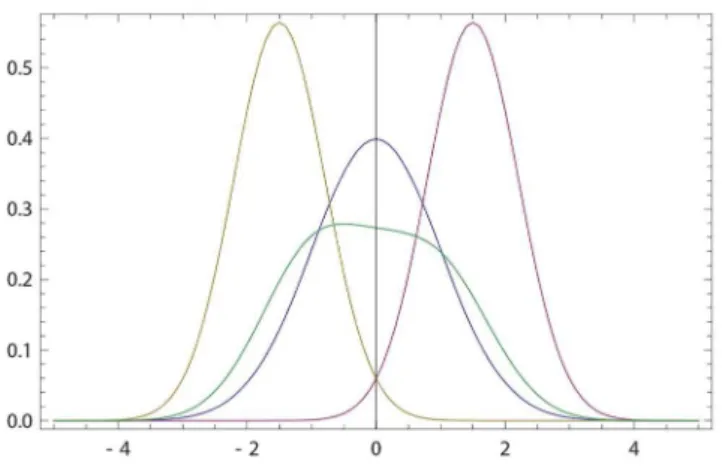
Figure 4. Order of presentation effect. Blue curve: The initial opinion of P is described by Gaussian probability density p(x) with

m_P~0andv_P~1; see (17). Purple (resp. olive) curve: the initial opinion ofQ(resp.Q’_{) are given by (17) with}m_Q~1:5(resp.m_Q’~{1:5) and v_Q~0:5(resp.v_Q’~0:5). Green curve: the resulting opinion ofPafter interacting first withQand then withQ’_{. Both interactions use}E~0:5. The final opinion ofPis inclined to the most recent opinion (that ofQ’₎ both with respect to its maximally probable value and distance. The final opinion ofPhas a larger width than the initial one.

doi:10.1371/journal.pone.0099557.g004

zg 2

4(pk{qk)zO½g 3

: _ð38_Þ

Hence in this limitpk(q,q’){pk(q’,q)depends only onq’k{qk

(and not e.g. onql6~k):

pk(q,q’){pk(q’,q)~g2½q’k{qk=4zO½g3: ð39Þ

It is seen that the more probable persuasive opinion (e.g. the opinion of_Q’ifq’_kwqk) changes the opinion ofPif it comes later.

This implies the recency effect. Indeed, due to symmetry conditions for checking the order of presentation effect we can also look at h½p(q,q’),q{h½p(q’,q),q. Using (39) we get for this

quantity: g

2

16h½p(q’_,q),q X

k

½qk{q’k

ffiffiffiffiffiffiffiffiffiffiffiffi qk=pk

p

w0, again due to

symmetry conditions.

Note that this argument on recency directly extends to more general situations, where the agent is exposed to different opinions multiple times. For instance, consider an exposure sequence q q q’_q’_{and its reverseq}’_q’_{q q. It can be shown that the model} predicts a recency effect in this scenario as well. For this case, we get instead of (39):pk(q,q’){pk(q’,q)~g2½q’k{qkzO½g3.

Note that the primacy-recency effect is only one (though important!) instance of contextual and non-commutative phenom-ena in psychology; see [11,66] and references therein. Hence in section IV of File S1 we study a related (though somewhat less interesting) order of presentation effect, while below we discuss our findings in the context of experimental results.

Experimental studies of order of presentation effect We now discuss our findings in this section in the context of experimental results on primacy and recency. The latter can be roughly divided into several group: persuasion tasks [10,50], symbol recalling [70], inference tasks [34], and impression formation [7,9]. In all those situations one generally observes both primacy and recency, though in different proportions and under different conditions [34]. Generally, the recency effect is observed whenever the retention time (the time between the last stimulus and the data taking) is short. If this time is sufficiently long, however, the recency effect changes to the primacy effect [10,50,62,70]. The general interpretation of these results is that there are two different processes involved, which operate on different time-scales. These processes can be conventionally related to short-term and long-term memory [70], with the primacy effect related to the long-term memory. In our model the longer time process is absent. Hence, it is natural that we see only the recency effect. The prevalence of recency effects is also seen in inference tasks, where the analogue of the short retention time is the incremental (step-by-step) opinion revision strategy [34].

At this point, let us remind the importance of symmetry conditions [such as (34)] for observing a genuine order of presentation effect. Indeed, several experimental studies–in particular those on impression formation–suggest that the order of presentation existsdueto different conditions in the first versus the second interaction [7,10,34,68,]. (In our context, this means different parametersE and E’for each interaction). For instance, Refs. [7,10] argue that the primacy effect is frequently caused by attention decrement (the first action/interaction gets more

attention); see also [68] in this context. This effect is trivially described by our model, if we assumeEto be sufficiently smaller thanE’. In related experiments, it was shown that if the attention devoted to two interactions is balanced, the recency effect results [33], which is consistent with the prediction of our model.

At the same time, in another interesting study based on subjective probability revision, where the authors had taken special measures for minimizing the attention decrement, the results indicated a primacy effect [55].

We close this section by underlining the advantages and drawbacks of the present model concerning the primacy-recency effect: the main advantage is that it demonstrates the recency effect and shows that the well-known argument on relating confirmation bias to primacy does not hold generally. The main drawback is that the model does not involve processes that are supposedly responsible for the experimentally observed interplay between recency and primacy. In the concluding section we discuss possible extensions of the model that can account for this interplay.

Cognitive Dissonance

Consider an agent whose opinion probability density has two peaks on widely separated events. Such a density–with the most probable opinion being different from the average–is indicative of cognitive dissonance, where the agent believes in mutually conflicting things [10,26].

The main qualitative scenario for the emergence of cognitive dissonance is when an agent–who initially holds a probabilistic opinion with a single peak–is exposed to a conflicting information coming from a sufficiently credible source [10,26]. We now describe this scenario quantitatively.

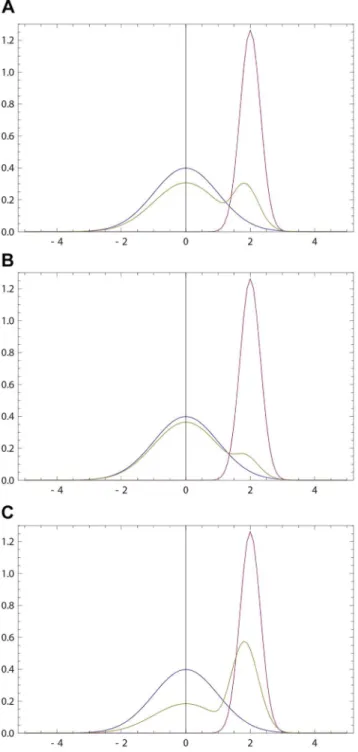
Consider again the opinion revision model (16, 17), and assume thatDm_P{m_QDis neither very large nor very small (in both these cases no serious opinion change is expected), v_Q=v_Pv1 (self-assured persuasive opinion) and0vEv1. In this case, we get two peaks (anchors) for the final density~pp(x). The first peak is very close to the initial anchor ofp(x), while the second closer to the anchor of q(x); see Fig. 5(a). Thus, persuasion from _Q whose opinion is sufficiently narrow and is centered sufficiently close (but not too close) to_P’s initial anchor leads to cognitive dissonance:_P holds simultaneously two different anchors, the old one and the one induced byQ.

There are 3 options for reducing cognitive dissonance: (i)IncreaseEmaking it closer to 1, i.e. making_Qless credible; see Fig. 5(b).

(ii)Decrease the width of the initial opinion ofP.

(iii)DecreaseE makingQmore credible. In this last case, the second peak of ~pp(x) (the one close to the anchor ofQ) will be dominant; see Fig. 5(c).

To understand the mechanism of the cognitive dissonance as described by this model, let us start from (1) and assume for simplicity that the opinion ofQis certain:qk~0fork~6 l and

ql~1. We get from (13):

e pk

pk~

pk

1{plzpl

ffiffiffiffiffiffiffiffiffiffiffiffiffiffiffiffiffiffiffiffiffiffiffiffiffiffiffiffi Ez_ð1{E_Þp{1

l

q fork=l, ð40Þ

~

p pl~

pl

ffiffiffiffiffiffiffiffiffiffiffiffiffiffiffiffiffiffiffiffiffiffiffiffiffiffiffi Ez(1{E)p{1

l

q

1{plzpl

ffiffiffiffiffiffiffiffiffiffiffiffiffiffiffiffiffiffiffiffiffiffiffiffiffiffiffi Ez(1{E)p{1

l

Now~ppl=plw1wpp~k=pk, wherek~6 l; hence even iflwas on the

tail of_fpkgNk~1, it is possible to make it a local (or even the global) maximum of_f~ppkgNk~1provided thatEis not close to 1.

The existence of at least two widely different probable opinions is only one aspect of cognitive dissonance [10,26]. Another aspect (sometimes called Freud-Festinger’s law) is that people tend to avoid cognitive dissonance: if in their action they choose one of the two options (i.e. one of two peaks of the subjective probability), they re-write the history of their opinion revision so that the chosen option becomes the most probable one [10,26]. This aspect of cognitive dissonance found applications in economics and decision making [2,73]. The above points(i)–(iii)provide concrete scenarios for a such re-writing.

Repeated Persuasion

Here we analyze the opinion dynamics under repeated persuasion attempts. Our motivation for studying this problem is that repeated exposure to the same opinion is generally believed to be more persuasive than a single exposure.

Under certain conditions (pkqk=0, for allk and1wEw0) we

show that the target opinion converges to the persuading opinion after sufficient number of repetition. Below we also examine how exactly this convergence takes place.

Assume that _P revises his opinion repeatedly with the same opinion ofQ. Eq. (13) implies (1ƒkƒN)

p½_knz1~

ffiffiffiffiffiffiffiffiffiffiffiffiffiffiffiffiffiffiffiffiffiffiffiffiffiffiffiffiffiffiffiffiffiffiffiffiffiffiffiffiffi p½_kn_½Ep_k½nz(1{E)qk)

q

PN l~1

ffiffiffiffiffiffiffiffiffiffiffiffiffiffiffiffiffiffiffiffiffiffiffiffiffiffiffiffiffiffiffiffiffiffiffiffiffiffiffiffi p½_ln½Ep_l½nz(1{E)ql)

q , ð42Þ

where1wEw0, andn~1,2,:::is the discrete time. For simplicity, we assume

p½ _k1:_pkw0,qkw0 for 1ƒkƒN: ð43Þ

Eq. (42) admits only one fixed pointq~_fqkgNk~1. Section VI of

File S1 shows that for any convex,d 2_f(y)

dy2 §0, functionf(y) one has

W½p½nz1_;qƒW½p½n_{;q, ð44Þ}

W½p;q: XN

k~1qkf(pk=qk):

ð45_Þ

HenceW½p;qis a Lyapunov function of (42). SinceW½p;qis a convex function ofp,W½p;q§f(1)~_W½q;qandf(1) is the unique global minimum ofW½p;q. Section VI of File S1 shows that the equality sign in (45) holds ony for p½nz1~p½n. Thus W½p½n;q

monotonically decays tof(1)~_W½q;qshowing that the fixed point q is globally stable. More generally, the convergence reads:

p½_kn?f_½p½_k1qk=

XN

l~1f½p ½1

l ql, wheref(xw0)~1andf(0)~0.

To illustrate (44, 45), one can take f(y)~{pffiffiffiy. Then (44) amounts to decaying Hellinger distance (30). Many other reasonable measures of distance are obtained under various choices off. For instance,f(y)~Dy{1Damounts to decaying total variation distance (33), whilef(y)~{lnyleads to the decaying relative entropy (Kullback-Leibler entropy).

As expected, 0vEv1 influences the convergence time. We checked that this time is an increasing function ofE, as expected. Figure 5. Cognitive dissonance.(a) Blue (resp. purple) curve: the

initial opinion of agentP(resp.Q) described by probability densityp(x) (resp.q(x)). Olive curve: the final opinion~pp(x)ofPas given by (16) with

E~0:35. Herep(x) and q(x) are defined by (17) with m_P~0, v_P~1,

m_Q~2,v_Q~0:1. The final opinion develops two peaks of comparable height (cognitive dissonance). (b) Avoiding the cognitive dissonance due to a larger E~0:75: the second peak is much smaller (other parameters are those of (a)). (c) Avoiding the cognitive dissonance due to a smallerE~0:05: the first peak is much smaller (other parameters are those of (a)).

In section VI of File S1 we also show that the convergence to the fixed point respects the Le Chatelier principle known in thermodynamics [4]: the probabilities of those events that are overestimated from the viewpoint of_Q(i.e.p½_k1wqk) tend to decay

in the discrete time. Likewise, probabilities of the underestimated events (i.e.p½_k1vqk) increase in time.

Let us consider the Hellinger distancehn~h½p½nz1,p½nbetween

two consecutive opinions ofPevolving as in (42). It is now possible that

max1ƒnv?½hn~hm6~h1, ð46Þ

i.e. the largest change of the opinion ofPcomes not from the first, but from one of intermediate persuasions. A simple example of this situation is realized for N = 3, an initial probability vector p~(0:98,0:01,0:01) and q~(0:01,0:01,0:98) in (43). We then apply (42) underE~0:5. The consecutive Hellinger distances read h1~0:1456vh2~0:1567wh3~0:1295wh4:::. Hence the second persuasion changes the opinion more than others. For this to hold, the initial opinionpofP has to be far from the opinionqofQ. Otherwise, we get a more expected behavior h1wh2wh3wh4::: meaning that the first persuasion leads to the largest change.

(The message of (46) is confirmed by using the discrete version

d½p,q~1

2 X

kDpk{qkD of the distance (33). Define dn~d½p½nz1,p½n. Then with p~(0:98,0:01,0:01) and

q~(0:01,0:01,0:98) we get d1~0:0834, d2~0:1636,

d3~0:1717,d4~0:1444.)

We conclude by stressing that while repeated persuasions drive the opinion to its fixed point monotonically in the number of repetitions, it is generally not true that the first persuasion causes the largest opinion change, i.e. the law of diminishing returns does not hold. To obtain the largest opinion change, one should carefully choose the number of repetitions.

Finally, note that the framework of (42) can be applied to studying mutual persuasion (consensus reaching). This is described in Section VII of File S1; see also [23] in this context.

Boomerang (Backfire) Effect

Definition of the effect

Theboomerangorbackfireeffect refers to the empirical observation that sometimes persuasion yields the opposite effect: the persuaded agent P moves his opinion away from the opinion of the persuading agent,Q, i.e. he enforces his old opinion [53,58,64,69]. Early literature on social psychology proposed that the boomerang effect may be due to persuading opinions placed in the latitude of rejection [69], but this was not confirmed experimentally [40].

Experimental studies indicate that the boomerang effect is frequently related with opinion formation in an affective state, where there are emotional reasons for (not) changing the opinion. For example, a clear evidence of the boomerang effect is observed when the persuasion contains insulting language [1]. Another interesting example is when the subjects had already announced their opinion publicly, and were not only reluctant to change it (as for the usual conservatism), but even enforced it on the light of the contrary evidence [64] (in these experiments, the subjects who did not make their opinion public behaved without the boomerang effect). A similar situation is realized for voters who decided to support a certain candidate. After hearing that the candidate is criticized, the voters display a boomerang response to this criticism and thereby increase their support [53,58].

Opinion revision rule

We now suggest a simple modification of our model that accounts for the basic phenomenology of the boomerang effect.

Recall our discussion (around (8)) of various psychological and social factors that can contribute into the weightE. In particular, increasing the credibility of_Qleads to a larger1{E. Imagine now that_Qhas such a low credibility that

Ew1: ð47Þ

Recall that E~1 means a special point, where no change of opinion of_P is possible whatsoever; cf. (13).

After analytical continuation of (13) for Ew1, the opinion revision rule reads

~

p pk~

ffiffiffiffiffiffiffiffiffiffiffiffiffiffiffiffiffiffiffiffiffiffiffiffiffiffiffiffiffiffiffiffiffiffiffi pkDEpkz(1{E)qkD

p PN

l~1

ffiffiffiffiffiffiffiffiffiffiffiffiffiffiffiffiffiffiffiffiffiffiffiffiffiffiffiffiffiffiffiffiffi plDEplz(1{E)qlD

p , ð48Þ

with obvious generalization to probability densities. The absolute values in (48) are necessary to ensure the positivity of probabilities.

It is possible toderive(rather simply postulate) (48). Toward this end, let us return to the point 6.1and (8). During the opinion combination step,P formsEpkz(1{E)qk which in view ofEw1

can take negative values and hence is a signed measure. Signed measures have all formal features of probability besides positivity [6,14,19,65]; see section V of File S1 for details. There is no generally accepted probabilistic interpretation of signed measures, but in section V of File S1 we make a step towards such an interpretaion. There we propose to look at a signed measure as a partial expectation value defined via joint probability of the world’s states and certain hidden degrees of freedom (e.g. emotional states). After plausible assumptions, the marginal probability of the world’s states is deduced to be

Figure 6. Opinion change in the boomerang regime.Blue (resp. purple) curve: the initial opinion of agentP (resp. Q) described by probability densityp(x) (resp.q(x)). Olive curve: the final opinion~pp(x)of Pgiven by (16) withE~2. Herep(x) andq(x) are given by (17) with

m_P~0andv_P~m_Q~v_Q~1. The anchor (maximally probable opinion) ofPnot only moves away from the anchor ofQ; but it is also enhanced: the (biggest) peak of~pp(x)is larger than that ofp(x). The second (smaller) peak of~pp(x)arises because the initial probability ofPlocated to the right from the anchorm_QofQ, moves away fromm_Q;~pp(x)gets a local minimum close tom_Q.

^

p

pk~DEpkz(1{E)qkD=

XN

l~1

DEpkz(1{E)qkD, ð49Þ

We obtain (48) after applying (9, 10) to (49).

Scenarios of opinion change

According to (47, 48) those opinions ofPwhich are within the overlap between p and q (i.e pkqk&6 0) get their probability

decreased ifpk=qk&(E{1)=Ev1, i.e. if the initialpkwas already smaller thanqk. In this sense,Pmoves his opinion away from that ofQ. Hence for continuous densitiesp(x) andq(x) there will be a pointx0, where~pp(x0)is close to 0. This point is seen in Figs. 6 and

7.

Fig. 6 illustrates the shape of~pp(x)produced by (48) for initially Gaussian opinions (17) of _P and _Q. It is seen that _P’s anchor moves away from_Q’s anchor, while the width of~pp(x)around the anchor is more narrow than that of p(x); cf. with Fig. 4. To illustrate these points analytically, we return to (29, 24, 24) that for

vP&vQ and mP&mQ predict m_PPe{mP~1 {E

2 (mQ{mP): for Ew1,_P’s anchor drifts away from_Q’s anchor.

Likewise, whenever the two anchors are equal, mP~mQ, inequality (27) is reversed in the boomerang regime (47).

Let us now consider the impact of the presentation order under this settings. We saw that for0vEv1the model predicts recency effect. For 1*Ewe expect the recency effect is still effective as

implied by the argument (39). However, the situation changes drastically for Esufficiently larger than 1, as indicated in Fig. 7. Now the primacy effect dominates, i.e. instead of (35) we get the opposite inequality. Fig. 7 also shows that interaction with two contradicting opinions (in the boomerang regime) enforces the initial anchor of_P.

To understand the primacy-recency effect analytically, consider the example (36), and recall that_Pinteracts first with_Qand then with_Q’with the same parameterE. The resulting opinionp(q,q’₎ of_Preads:

p(q,q’₎~ g(E) g(E)z1,

1 g(E)z1

, ð50Þ

g(E)~

ffiffiffiffiffiffiffiffiffiffiffiffiffiffiffiffiffiffiffiffiffiffiffiffiffiffiffiffiffiffiffiffiffiffiffiffiffiffiffiffiffiffi_ffiffi E

p_z(1{E) ffiffiffiffiffiffiffiffiffiffiffiffi D2{ED

p

ffiffi E

p (2{E)

s

ð51_Þ

Fig. 8 shows howp1(q,q’₎~ g(E)

g(E)z1 behaves as a function ofE. The recency effect holds for Ev2zpffiffiffi₂; for Ew2zpffiffiffi₂ we get primacy. Similar results are obtained for initially Gaussian opinions.

Thus, in the present model, the primacy effect (relevance of the first opinion) can be related to the boomerang effect.

We now examine the emergence of cognitive dissonance in the boomerang regimeEw1. Our results indicate that in this regime the agent is more susceptible to cognitive dissonance; cf. Fig. 6 with Figs. 1. The mechanism of the increased susceptibility is explained in Fig. 6:_P’s opinion splits easier, since the probability mass moves away (in different directions) from the anchor of_Q.

Let us now assume that_P repeatedly interacts with the same opinion of_Q[cf. (42)]:

p½nz1(x)~

ffiffiffiffiffiffiffiffiffiffiffiffiffiffiffiffiffiffiffiffiffiffiffiffiffiffiffiffiffiffiffiffiffiffiffiffiffiffiffiffiffiffiffiffiffiffiffiffiffiffiffiffiffiffiffi p½n_(x)DEp½n_(x)z(1{E)q(x)D p

Ð

dx’pffiffiffiffiffiffiffiffiffiffiffiffiffiffiffiffiffiffiffiffiffiffiffiffiffiffiffiffiffiffiffiffiffiffiffiffiffiffiffiffiffiffiffiffiffiffiffiffiffiffiffiffiffiffiffiffiffiffi_p½n_(x’_)DEp½n_(x’₎z(1{E)q(x’₎D, ð52Þ

where n~1,2,::: is the discrete time. Starting from initially Gaussian opinion,_P develops two well-separated peaks, which is another manifestation of cognitive dissonance: the smaller peak moves towards the anchor ofQand finally places itself within the acceptance latitude of _Q, where the larger peak becomes more narrow and drifts away fromq(x); see Fig. 9. After many iterations (^103_{for parameters of Fig. 9) the larger peak places itself within} the rejection latitude of_Q, at which pointp½n(x)stops changing (stationary opinion). The above scenario suggests that in the boomerang regime there is a finite probability that the target agent Figure 7. Order of presentation effect in the boomerang

regime. The same as in Fig.4 but forE~1:5(boomerang regime). Now the final opinion ofPis inclined to the first opinion (that ofQ) with respect to the distance. The initial maximally probable opinion of P is still maximally probable. Moreover, its probability has increased and the width around it has decreased. The final opinion has 3 peaks. doi:10.1371/journal.pone.0099557.g007

Figure 8. Illustration of the order of presentation effect in the

boomerang regime.p1(q,q’)~ g(E)

g(E)z1 given by (50, 51) versusE. doi:10.1371/journal.pone.0099557.g008

will eventually be persuaded after repeated exposure to the same opinion.

Let us mention an experimental work that is relevant to our discussion above. Ref. [58] carried out experiments with subjects displaying boomerang effect, where each subject was exposed to sufficiently many different (but still similar) persuasive opinions. It was found that, sooner or later, the subjects exit the boomerang regime, i.e. they start to follow the persuasion [58]. Our set-up is somewhat different in that the subject (_P) is repeatedly exposed to the same persuading opinion. Modulo this difference, our conclusion is similar to the experimental finding: the agent starts following the persuasion with a certain probability.

Discussion

We presented a new model for opinion revision in the presence of confirmation bias. The model has three inputs: the subjective probabilistic opinions of the target agent P and a persuading (advising) agent_Q, and the weight of_Qas perceived by_P.

The basic idea of the opinion revision rule is that no opinion change is expected if the persuasion is either too far or too close to the already existing opinion [15,36,60]. The opinion revision rule is not Bayesian, because the standard Bayesian approach does not apply to processes of persuasion and advising; see the second section for more details.

The model accounts for several key empirical observations reported in social psychology and quantitatively interpreted within the social judgment theory. In particular, the model allows to formalize the concept of opinion latitudes, explains the structure of the weighted average approach to opinion formation, and relates the initial discrepancy (between the opinions ofP andQ) to the magnitude of the opinion change (shown by_P). In all these cases our model extends and clarifies previous empiric results, e.g. it elucidates the difference between monotonic and non-monotonic change-discrepancy relations, identifies conditions under which the opinion change is sudden, as well as provides a deeper perspective on the weighted average approach.

New effects predicted by the model are summarized as follows. (i) For the order of presentation set-up (and outside of the boomerang regime) the model displays recency effect. We suggested that the standard argument that relates confirmation

bias to the primacy effect does not work in this model. In this context we recall a widespread viewpoint thatboth recency and primacy relate to (normative) irrationality; see e.g. [13]. However, the information which came later is generally more relevant for predicting future. Hence recency can be more rational than primacy.

In many experimental set-ups the recency changes to primacy upon increasing the retention time; see e.g. [70]. Our model demonstrates the primacy effect only in the boomerang regime (i.e. only in the special case). Hence, in future it needs to be extended by involving additional mechanisms, e.g. those related to ‘‘long-term memory’’ processes which could be responsible for the above experimental fact. Recall in this context there are several other theoretical approaches that address the primacy-recency difference [11,34,42,56,66].

(ii) The model can be used to describe the phenomenon of cognitive dissonance and to formalize the main scenario of its emergence.

(iii) Repeated persuasions display several features implying monotonous change of the target opinion towards the persuading opinion. However, the opinion changes do not obey the law of diminishing returns, or in other words, the first persuasion is not always leads to the largest change. These findings may contribute to better understanding the widespread use of repeated persua-sions.

(iv)We proposed that the boomerang effect is related to the limit of this model, where the credibility of persuasion is (very) low. A straightforward implementation of this assumption led us to a revision rule that does describe several key observational features of the boomerang effect and predicts new ones; e.g. that in the boomerang regime the agent can be prone to primacy effect and to cognitive dissonance. There are, however, several open problems with the opinion revision rule in the boomerang regime. They should motivate future developments of this model. One problem concerns relations of the revision rule with signed measures that at a preliminary level were outlined in section V of File S1. Another problem is that the revision rule in the boomerang regime (and only there) is not completely smooth, since it includes the function DxD, whose second derivative is singular. We do hope to clarify these points in future.

In this paper we restricted ourselves by studying few (two or three) interacting agents with opinions described via subjective probabilities. However, these probabilities can also represent an ensemble of agents each one having a fixed (single) opinion, a useful viewpoint on subjective probabilities advocated in Ref. [37]. In future we plan to explore this point and also address the opinion dynamics for collectives of agents. This last aspect was recently extensively studied via methods of statistical physics; see [20,63] for reviews.

Supporting Information

File S1 (PDF)

Acknowledgments

We thank Seth Frey for useful remarks and suggestions.

Author Contributions

Conceived and designed the experiments: AA AG. Performed the experiments: AA. Analyzed the data: AA AG. Wrote the paper: AA.

Figure 9. Repeated persuasion in the boomerang regime.Blue (resp. purple) curve: the initial opinion of agentP(resp.Q) described by probability density p(x) (resp. q(x)) as given by (17) with m_P~0,

v_P~vQ~1,mQ~1. Olive curve: the opinion ofPafter 50 iterations (52) withE~2.