No 650 ISSN 0104-8910
A Panel Data Approach to Economic
Forecasting: The Bias–Corrected Average
Forecast
Os artigos publicados são de inteira responsabilidade de seus autores. As opiniões
neles emitidas não exprimem, necessariamente, o ponto de vista da Fundação
A Panel Data Approach to Economic Forecasting:
The Bias-Corrected Average Forecast
João Victor Issler and Luiz Renato Limay
Graduate School of Economics – EPGE Getulio Vargas Foundation email: [email protected] and [email protected]
First Draft: December, 2006. Revised: September, 2007.
Abstract
In this paper, we propose a novel approach to econometric forecast-ing of stationary and ergodic time series within a panel-data frame-work. Our key element is to employ the (feasible) bias-corrected aver-age forecast. Using panel-data sequential asymptotics we show that it is potentially superior to other techniques in several contexts. In partic-ular, it is asymptotically equivalent to the conditional expectation, i.e., has an optimal limiting mean-squared error. We also develop a zero-mean test for the average bias and discuss the forecast-combination puzzle in small and large samples. Monte-Carlo simulations are con-ducted to evaluate the performance of the feasible bias-corrected aver-age forecast in …nite samples. An empirical exercise, based upon data
We are especially grateful for the comments and suggestions given by two anonymous referees, Marcelo Fernandes, Wagner Gaglianone, Antonio Galvão, Ra¤aella Giacomini, Clive Granger, Roger Koenker, Marcelo Medeiros, Marcelo Moreira, Zhijie Xiao, and Hal White. We also bene…ted from comments given by the participants of the conference “Econometrics in Rio.” We thank Wagner Gaglianone and Claudia Rodrigues for excellent research assistance and gratefully acknowledge the support given by CNPq-Brazil, CAPES, and Pronex. João Victor Issler thanks the hospitality of the Rady School of Management, and the Department of Economics of UCSD, where parts of this paper were written. Both authors thank the hospitality of University of Illinois, where the …nal revision was written. The usual disclaimer applies.
from a well known survey is also presented. Overall, these results show promise for the feasible bias-corrected average forecast.
Keywords: Forecast Combination, Forecast-Combination Puzzle, Com-mon Features, Panel-Data, Bias-Corrected Average Forecast.
J.E.L. Codes: C32, C33, E21, E44, G12.
1
Introduction
Bates and Granger(1969) made the econometric profession aware of the ben-e…ts of forecast combination when a limited number of forecasts is consid-ered. The widespread use of di¤erent combination techniques has lead to an interesting puzzle from the econometrics point of view – the well known fore-cast combination puzzle: if we consider a …xed number of forecasts(N <1), combining them using equal weights(1=N) fare better than using “optimal weights” constructed to outperform any other forecast combination in the mean-squared error (MSE) sense.
Regardless of how one combine forecasts, if the series being forecast is stationary and ergodic, and there is enough diversi…cation among forecasts, we should expect that a weak law-of-large-numbers (WLLN) applies to well-behaved forecast combinations. This argument was considered in Palm and Zellner (1992) who asked the question “to pool or not to pool” forecasts? Recently, Timmermann (2006) used risk diversi…cation – a principle so keen in …nance – to defend pooling of forecasts. Of course, to obtain this WLLN result, at least the number of forecasts has to diverge (N ! 1), which entails the use of asymptotic panel-data techniques. In our view, one of the reasons why pooling forecasts has not yet been given a full asymptotic treatment, withN; T ! 1, is that forecasting is frequently thought to be a time-series experiment, not a panel-data experiment.
expectation of the series being forecast. Indeed, the latter is the common feature of all individual forecasts (Engle and Kozicki (1993)), while individ-ual forecasts deviate from the optimal because of forecast misspeci…cation; see the reasons listed in Palm and Zellner. Third, when N; T ! 1, and we use standard tools from panel-data asymptotic theory, we show that the pooling of forecasts delivers optimal limiting forecasts in the MSE sense. In our key result, we prove that, in the limit, the feasiblebias-corrected average forecast – equal weights in combining forecasts coupled with an estimated bias-correction term – is an optimal forecast identical to the conditional expectation.
The feasible bias-corrected average forecast is also parsimonious besides being optimal. The only parameter we need to estimate is the mean bias, for which we show consistency under the sequential asymptotic approach developed by Phillips and Moon (1999). Indeed, the only way we could increase parsimony in our framework is by doing without any bias correction. To test the usefulness of performing bias correction, we developed a zero-mean test for the average bias which draws upon the work of Conley (1999) on random …elds.
As a by-product of the use of panel-data asymptotic methods, with
N; T ! 1, we advanced the understanding of the forecast combination
puzzle. The key issue is that simple averaging requires no estimation of weights, while optimal weights requires estimatingN weights that grow un-bounded in the asymptotic setup. We show that there is no puzzle under certain asymptotic paths forN andT, but not for all. We fully characterize them here. We are also able to discuss the puzzle in small samples, linking its presence to the curse of dimensionality which plagues so many estimators throughout econometrics1.
Despite the scarcity of panel-data studies on the pooling of forecasts2,
there has been panel-data research on forecast focusing on the pooling of information; see Stock and Watson (1999 and 2002a and b) and Forni et al. (2000, 2003). Pooling forecasts is related to forecast combination and
1We thank Roger Koenker for suggesting this asymptotic exercise to us, and an
anony-mous referee for casting the puzzle in terms of the curse of dimensionality.
2The notable exception is Palm and Zellner (1992), who discuss “to pool or not to
operates a reduction on the space of forecasts. Pooling information operates a reduction on a set of highly correlated regressors. Forecasting can bene…t from the use of both procedures, since, in principle, both yield asymptoti-cally optimal forecasts in the MSE sense.
A potential limitation on the literature on pooling of information is that pooling is performed in a linear setup, and the statistical techniques em-ployed were conceived as highly parametric – principal-component and fac-tor analysis. That is a problem if the conditional expectation is not a linear function of the conditioning set or if the parametric restrictions used (if any) are too stringent to …t the information being pooled. In this case, pooling forecasts will be a superior choice, since the forecasts being pooled need not be the result of estimating a linear model under a highly restric-tive parameterization. On the contrary, these models may be non-linear, non-parametric, and even unknown to the econometrician, as is the case of using a survey of forecasts. Moreover, the components of the two-way de-composition employed here are estimated using non-parametric techniques, dispensing any distributional assumptions. This widens the application of the methods discussed in this paper.
Korajzcyk (1986), Phillips and Moon (1999), Bai and Ng (2002), Bai (2005), and Pesaran (2005). Indeed, our approach borrows form …nance the idea that we can only diversify idiosyncratic risk but not systematic risk. The lat-ter is associated with the common element of all forecasts – the conditional expectation term – which is to what a specially designed forecast average converges to.
The rest of the paper is divided as follows. Section 2 presents our main results and the assumptions needed to derive them. Section 3 presents the results of a Monte-Carlo experiment. Section 4 presents an empirical analy-sis using the methods proposed here, confronting the performance of our bias-corrected average forecast with that of other types of forecast combi-nation. Section 5 concludes.
2
Econometric Setup and Main Results
Suppose that we are interested in forecasting a weakly stationary and er-godic univariate process fytg using a large number of forecasts that will
be combined to yield an optimal forecast in the mean-squared error (MSE) sense. These forecasts could be the result of using several econometric mod-els that need to be estimated prior to forecasting, or the result of using no formal econometric model at all, e.g., just the result of an opinion poll on the variable in question using a large number of individual responses. We can also imagine that some (or all) of these poll responses are generated using econometric models, but then the econometrician that observes these forecasts has no knowledge of them.
Regardless of whether forecasts are the result of a poll or of the esti-mation of an econometric model, we label forecasts of yt, computed using
conditioning sets lagged h periods, by fh
i;t, i = 1;2; : : : ; N. Therefore, fi;th
areh-step-ahead forecasts andN is either the number of models estimated
to forecastyt or the number of respondents of an opinion poll regarding yt.
We consider 3 consecutive distinct time sub-periods, where time is in-dexed byt= 1;2; : : : ; T1; : : : ; T2; : : : ; T. The …rst sub-periodEis labeled the “estimation sample,” where models are usually …tted to forecast yt in the
labeled the post-model-estimation or “training sample”, where realizations ofyt are usually confronted with forecasts produced in the estimation
sam-ple, and weights and bias-correction terms are estimated, if that is the case. It hasR=T2 T1= 2 T observations in it, comprising (t=T1+1; : : : ; T2). The …nal sub-period isP (for prediction), where genuine out-of-sample fore-cast is entertained. It hasP =T T2 = 3 T observations in it, comprising (t = T2 + 1; : : : ; T). Notice that 0 < 1; 2; 3 < 1, 1 + 2 + 3 = 1, and that the number of observations in these three sub-periods keep a …xed proportion with T – respectively, 1, 2 and 3 – being all O(T). This is an important ingredient in our asymptotic results forT ! 1.
We now compare our time setup with that of West. He only considers two consecutive periods: R data points are used to estimate models and the subsequentP data points are used for prediction. His setup does not require estimating bias-correction terms or combination weights, so there is no need for an additional sub-period for estimating the models that generate the fh
i;t’s3. In the case of surveys, since we do not have to estimate models, our
setup is equivalent to West’s. Indeed, in his setup, R; P ! 1 asT ! 1,
and lim
T!1R=P = 2[0;1]. Here
4:
lim T!1
R
P =
2
3
= 2(0;1):
In our setup, we also let N go to in…nity, which raises the question of whether this is plausible in our context. On the one hand, if forecasts are the result of estimating econometric models, they will di¤er acrossiif they are either based upon di¤erent conditioning sets or upon di¤erent functional forms of the conditioning set (or both). Since there is an in…nite number of functional forms that could be entertained for forecasting, this gives an in…nite number of possible forecasts. On the other hand, if forecasts are the result of a survey, although the number of responses is bounded from above, for all practical purposes, if a large enough number of responses is obtained, then the behavior of forecast combinations will be very close to the limiting
behavior whenN ! 1.
3Notice that the estimated models generate the fh
i;t’s, but model estimation,
bias-correction estimation and weight estimation cannot be performed all within the same sub-sample in an out-of-sample forecasting exercise.
4To inlcude the supports of 2[0;1]we must, asymptotically, give up having either
Recall that, if we are interested in forecastingyt, stationary and ergodic,
using information up toh periods prior to t, then, under a MSE risk func-tion, the optimal forecast is the conditional expectation using information available up to t h: Et h(yt). Using this well-known optimality result,
Hendry and Clements (2002) argue that the fact that the simple forecast
average N1
N
X
i=1 fh
i;t usually outperforms individual forecasts fi;th shows our
inability to approximate Et h(yt) reasonably well with individual models.
However, since Et h(yt) is optimal, this is exactly what these individual
models should be doing.
With this motivation, our setup writes the fh
i;t’s as approximations to
the optimal forecast as follows:
fi;th =Et h(yt) +ki+"i;t, (1)
wherekiis the individual model time-invariant bias and"i;t is the individual
model error term in approximating Et h(yt). Here, the optimal forecast is
a common feature of all individual forecasts and ki and "i;t arise because
of forecast misspeci…cation5. We can always decompose the series y
t into
Et h(yt)and an unforecastable component t, such thatEt h( t) = 0in:
yt=Et h(yt) + t. (2)
Combining (1) and (2) yields,
fi;th = yt t+ki+"i;t, or,
fi;th = yt+ki+ t+"i;t, where, t= t: (3)
Equation (3) is indeed the well known two-way decomposition, or error-component decomposition, of the forecast errorfh
i;t yt:
fi;th = yt+ i;t i= 1;2; : : : ; N; t > T1; (4)
i;t = ki+ t+"i;t.
5If an individual forecast is the conditional expectation
Et h(yt), thenki ="i;t = 0.
Notice that this implies that its MSE is smaller than that of 1 N
N
X
i=1 fh
i;t, something that is
It has been largely used in econometrics dating back to Wallace and Hus-sein (1969), Amemiya (1971), Fuller and Battese (1974) and Baltagi (1980). Palm and Zellner (1992) employ a two-way decomposition to discuss fore-cast combination in a Bayesian and a non-Bayesian setup6, and Davies and Lahiri (1995) employed a three-way decomposition to investigate forecast rationality within the “Survey of Professional Forecasts.”
By construction, our framework in (4) speci…es explicit sources of fore-cast errors that are found in bothytandfi;th; see also the discussion in Palm
and Zellner and Davies and Lahiri. The termkiis the time-invariant forecast
bias of modelior of respondenti. It captures the long-run e¤ect of forecast-bias of modeli, or, in the case of surveys, the time invariant bias introduced by respondenti. Its source isfh
i;t. The term t arises because forecasters do
not have future information onybetweent h+ 1andt. Hence, the source of tisyt, and it is an additive aggregate zero-mean shock a¤ecting equally
all forecasts7. The term"i;t captures all the remaining errors a¤ecting
fore-casts, such as those of idiosyncratic nature and others that a¤ect some but not all the forecasts (a group e¤ect). Its source isfi;th.
From equation (4), we conclude that ki; "i;t and t depend on the …xed
horizon h. Here, however, to simplify notation, we do not make explicit this dependence on h. In our context, it makes sense to treat h as …xed and not as an additional dimension to i and t. In doing that, we follow West (1996) and the subsequent literature. As argued by Vahid and Issler (2002), forecasts are usually constructed for a few short horizons, since, as the horizon increases, the MSE in forecasting gets hopelessly large. Here,h will not vary as much asiand t, especially becauseN; T ! 18.
6Palm and Zellner show that the performance of non-Bayesian combinations obey the
following MSE rank: (i) the unfeasible weighted forecast with known weights performs better or equal to the simple average forecast, and (ii) the simple average forecast may perform better than the feasible weighted forecast with estimated weights. Our main result is that the feasible bias-corrected average forecast is optimal under sequential asymptotics. We also propose an explanation to the forecast-combination puzzle based on the curse of dimensionality. Critical to these results is the use of largeN; T asymptotic theory.
7Because it is a component ofy
t, and the forecast error is de…ned asfi;th yt, the forecast
error arising from lack of future information should have a negative sign in (4); see (3). To eliminate this negative sign, we de…ned t as the negative of this future-information
component.
8Davies and Lahiri considered a three-way decomposition withhas an added dimension.
From the perspective of combining forecasts, the componentski; "i;t and
tplay very di¤erent roles. If we regard the problem of forecast combination
as one aimed at diversifying risk, i.e., a …nance approach, then, on the one hand, the risk associated with "i;t can be diversi…ed, while that associated
with t cannot. On the other hand, in principle, diversifying the risk asso-ciated with ki can only be achieved if a bias-correction term is introduced
in the forecast combination, which reinforces its usefulness. We now list our set of assumptions.
Assumption 1 We assume thatki; "i;tand tare independent of each other
for alliand t.
Independence is an algebraically convenient assumption used throughout the literature on two-way decompositions; see Wallace and Hussein (1969) and Fuller and Battese (1974) for example. At the cost of unnecessary complexity, it could be relaxed to use orthogonal components, something we avoid here.
Assumption 2 ki is an identically distributed random variable in the
cross-sectional dimension, but not necessarily independent, i.e.,
ki i.d.(B; 2k); (5)
where B and 2k are respectively the mean and variance of ki. In
the time-series dimension, ki has no variation, therefore, it is a …xed
parameter.
The idea of dependence is consistent with the fact that forecasters learn from each other by meeting, discussing, debating, etc. Through their ongo-ing interactions, they maintain a current collective understandongo-ing of where their target variable is most likely heading to, and of its upside and downside risks. Given the assumption of identical distribution forki,B represents the
market (or collective) bias. Since we focus on combining forecasts, a pure
hbutkidoes not, the latter being critical to identifykiwithin their framework. Since, in
general, this restriction does not have to hold, our two-way decomposition is not nested into their three-way decompostion. Indeed, in our approach,ki varies with hand it is
idiosyncratic bias does not matter but a collective bias does. In principle, we could allow for heterogeneity in the distribution ofki – means and variances
to di¤er acrossi. However, that will be a problem in testing the hypothesis that forecast combinations are biased.
It is desirable to discuss the nature of the term ki, which is related to
the question of why we cannot focus solely on unbiased forecasts, for which ki = 0. The role ofki is to capture the long-run e¤ect, in the time
dimen-sion, of the bias of econometric models ofyt, or of the bias of respondenti.
A relevant question to ask is – why would forecasters introduce bias under a MSE risk function? Laster, Bennett and Geoum (1999), Patton and Tim-mermann (2006), and Batchelor (2007) list di¤erent arguments consistent with forecasters having a non-quadratic loss function9. The argument ap-plies for surveys and for models as well, since a forecaster can use a model that is unbiased and add a bias term to it. In the examples that follow, all forecasters employ a combination of quadratic loss and a secondary loss function. Bias is simply a consequence of this secondary loss function and of the intensity in which the forecaster cares for it. The …rst example is that of a bank selling an investment fund. In this case, the bank’s forecast of the fund return may be upward-biased simply because it may use this forecast as a marketing strategy to attract new clients for that fund. Although the bank is penalized by deviating from Et h(yt), it also cares for selling the shares
of its fund. The second example introduces bias when there is a market for
pessimism or optimism in forecasting. Forecasters want to be labelled as optimists or pessimists in a “branding” strategy to be experts on “worst-” or on “best-case scenarios,“worst-” respectively. Batchelor lists governments as examples of experts on the latter.
Assumption 3 The aggregate shock t is a stationary and ergodic M A
process of order at mosth 1, with zero mean and variance 2 <1.
Sincehis a bounded constant in our setup, tis the result of a cumulation of shocks toyt that occurred betweent h+ 1and t. Being anM A( )is a
9Palm and Zellner list additional reasons for bias in forecasts: carelessness; the use
of a poor or defective information set or incorrect model; and errors of measurement. Lack of information or of full knowledge of the data-generating process (DGP) ofyt will
consequence of the wold representation foryt and of (2). Ifytis already an
M A( )process, of order smaller thanh 1, then, its order will be the same of that of t. Otherwise, the order ish 1. In any case, it must be stressed that
tis unpredictable, i.e., thatEt h( t) = 0. This a consequence of (2) and of
the law of iterated expectations, simply showing that, from the perspective of the forecast horizonh, unless the forecaster has superior information, the aggregate shock t cannot be predicted.
Assumption 4: Let "t = ("1;t; "2;t; ::: "N;t)0 be a N 1 vector stacking
the errors"i;t associated with all possible forecasts. Then, the vector
process f"tg is assumed to be covariance-stationary and ergodic for
the …rst and second moments, uniformly on N. Further, de…ning as
i;t="i;t Et 1("i;t), the innovation of "i;t, we assume that
lim N!1
1
N2
N
X
i=1
N
X
j=1
E i;t j;t = 0: (6)
Non-ergodicity of"twould be a consequence of the forecastsfi;th beyond
ki. Of course, forecasts that imply a non-ergodic "t could be discarded.
Because the forecasts are computed h-steps ahead, forecast errors "i;t can
be serially correlated. Assuming that "i;t is weakly stationary is a way of
controlling its time-series dependence. It does not rule out errors displaying conditional heteroskedasticity, since the latter can coexist with the assump-tion of weak staassump-tionarity; see Engle (1982).
Equation (6) limits the degree of cross-sectional dependence of the er-rors "i;t. It allows cross-correlation of the form present in a speci…c group
of forecasts, although it requires that this cross-correlation will not pre-vent a weak law-of-large-numbers from holding. Following the forecasting literature with large N and T, e.g., Stock and Watson (2002b), and the …nancial econometric literature, e.g., Chamberlain and Rothschild (1983), the condition lim
N!1
1
N2
PN
i=1
PN
j=1 E i;t j;t = 0 controls the degree of
cross-sectional decay in forecast errors. It is noted by Bai (2005, p. 6), that Chamberlain and Rothschild’s cross-sectional error decay requires:
lim N!1
1
N
N
X
i=1
N
X
j=1
Notice that this is the same cross-sectional decay used in Stock and Watson. Of course, (7) implies (6), but the converse is not true. Hence, Assumption 2 has a less restrictive condition than those commonly employed in the literature of factor models.
We state now basic results related to the classic question of “to pool or not to pool forecasts,” when only simple weights (1=N) are used; see, for example, Granger (1989) and Palm and Zellner (1992).
Proposition 1 Under Assumptions 1-4, the mean-squared error in fore-castingyt, using the individual forecast fi;th, isE fi;th yt
2
=ki2+ 2+ 2i, where 2i is the variance of "i;t,i= 1;2; ; :::; N.
Proof. Start with:
fi;th yt=ki+ t+"i;t.
Then, the MSE of individual forecasts is:
M SEi = E fi;th yt
2
=E(ki+ t+"i;t)2 (8)
= E k2i +E 2t +E "2i;t
= ki2+ 2+ 2i;
where 2i is the variance of "i;t. Assumption 1 is used in the second line of
(8). We also use the fact thatki is a constant in the time-series dimension
in the last line of (8).
Proposition 2 Under Assumptions 1-4, as N ! 1, the mean-squared er-ror in forecasting yt, combining all possible individual forecasts fi;th, is
M SEaverage =E plim N!1
1
N N
X
i=1 fh
i;t yt
!2
=B2+ 2.
Proof. Start with the cross-sectional average of (4):
1
N
N
X
i=1
fi;th yt= 1
N
N
X
i=1
ki+ t+ 1
N
N
X
i=1 "i;t.
Computing the probability limit of the right-hand side above gives,
plim
N!1
1
N
N
X
i=1
ki+ t+ plim
N!1
1
N
N
X
i=1
We will compute the probability limits in (9) separately. The …rst one is a straightforward application of the law of large numbers:
plim N!1 1 N N X i=1
ki=B.
The second will turn out to be zero. Our strategy is to show that, in
the limit, the variance of N1
N
X
i=1
"i;t is zero, a su¢cient condition for a weak
law-of-large-numbers to hold forf"i;tgNi=1.
Because"i;t is weakly stationary and mean-zero, for everyi, there exists
a scalar wold representation of the form:
"i;t=
1 X
j=0
bi;j i;t j (10)
where, for alli,bi;0= 1,Pj1=0b2i;j <1, and i;t is white noise.
In computing the variance of N1
N X i=1 1 X j=0
bi;j i;t j we use the fact that
there is no cross correlation between i;t and i;t k,k= 1;2; : : :. Therefore, we need only to consider the sum of the variances of terms of the form
1
N
PN
i=1bi;k i;t k. These variances are given by:
VAR 1
N
N
X
i=1
bi;k i;t k
! = 1 N2 N X i=1 N X j=1
bi;kbj;kE i;t j;t ; (11)
due to weak stationarity of "t. We now examine the limit of the generic
term in (11) with detail:
VAR 1
N
N
X
i=1
bi;k i;t k
! = 1 N2 N X i=1 N X j=1
bi;kbj;kE i;t j;t
1 N2 N X i=1 N X j=1
bi;kbj;kE i;t j;t = 1 N2 N X i=1 N X j=1
jbi;kbj;kj E i;t j;t (12)
max
i;j jbi;kbj;kj 1 N2 N X i=1 N X j=1
E i;t j;t :
Hence:
lim N!1VAR
1
N
N
X
i=1
bi;k i;t k
!
lim
N!1 maxi;j jbi;kbj;kj lim
N!1
1
N2
N
X
i=1
N
X
j=1
E i;t j;t = 0;
since the sequencefbi;jg1j=0is square-summable, yielding lim
N!1 maxi;j jbi;kbj;kj <
1, and Assumption 4 imposes lim N!1
1
N2
PN
i=1
PN
j=1 E i;t j;t = 0.
Thus, all variances are zero in the limit, as well as their sum, which gives:
plim
N!1
1
N
N
X
i=1
"i;t = 0:
Therefore,
E plim
N!1
1
N
N
X
i=1
fi;th yt
!2
= E(B+ t)2
= B2+ 2: (14)
We can now compare the MSE of a generic individual forecast with that of an equally weighted(1=N) forecast combination by using the usual bias-variance standard decomposition of the mean squared error (MSE)
M SE=Bias2+V AR.
Proposition 1 shows that we can decompose individual MSE’s, M SEi,
as:
M SEi = k2i + 2+ 2i
= Bias2i +V ARi,i= 1;2; :::; N
where Bias2
i = k2i and V ARi = 2 + 2i. Proposition 2 shows that
averaging forecasts reduces variance, but not necessarily MSE,
M SEaverage = B2+ 2 (15)
whereV ARaverage = 2 < V ARi = 2+ 2i, but comparing Bias2average =
B2 withBias2
i =ki2 requires knowledge of B and ki, which is also true for
comparing M SEaverage with M SEi. If the mean bias B = 0, i.e., we are
considering unbiased forecasts, on average, thenM SEi =ki2+ 2+ 2i, while
M SEaverage = 2. Therefore, if the number of forecasts in the combination
is large enough, combining forecasts with a zero collective bias will lead to a smaller MSE – as concluded in Granger (1989). However, if B 6= 0, we cannot conclude that the average forecast has MSE lower than that of individual forecasts, sinceB2 may be larger or smaller than ki2+ 2i.
This motivates studying bias-correction in forecasting, since one way to eliminate the term B2 in (14) is to perform bias correction coupled with equal weights (1=N) in the forecast combination. The next set of results investigates the properties of the bias-corrected average forecast (BCAF).
Proposition 3 If Assumptions 1-4 hold, then, the bias-corrected average forecast, given by N1
N
X
i=1 fh
i;t N1 N
X
i=1
ki, obeys plim N!1 1 N N X i=1 fh
i;t N1 N X i=1 ki ! =
yt+ t and has a mean-squared error as follows:
M SEBCAF = E
" plim N!1 1 N N X i=1 fh
i;t N1 N X i=1 ki ! yt #2
= 2. Therefore, it
is an optimal forecasting device in the MSE sense.
Proof. From the proof of Proposition 2, we have:
plim N!1 1 N N X i=1
fi;th yt plim N!1 1 N N X i=1
ki = t+ plim
N!1 1 N N X i=1 "i;t
= t;
leading to: E " plim N!1 1 N N X i=1
fi;th 1 N N X i=1 ki ! yt #2
= 2:
idiosyncratic components and group e¤ects. The only term left in the MSE is 2, related to unforecastable news to the target variable after the forecast combination was computed – something we could not eliminate unless we had superior (future) information. From a …nance perspective, all risks associated with terms that could be diversi…ed were eliminated by using the bias-corrected average forecast. We were left only with the undiversi…able risk expressed in 2. Therefore, the optimal result.
There are in…nite ways of combining forecasts. So far, we have considered only equal weights1=N. In order to discuss the forecast-combination puzzle, we now consider other combination schemes, consistent with a weak law-of-large-numbers for forecast combinations, i.e., bounded weights that add up to unity, in the limit.
Corollary 4 Consider the sequence of deterministic weights f!igNi=1, such
thatj!ij<1 uniformly on N and lim N!1
N
X
i=1
!i = 1. Then, under
Assump-tions 1-4,
plim
N!1
N
X
i=1 !ifi;th
N
X
i=1
!iki yt
!
= t; and,
E "
plim
N!1
N
X
i=1 !ifi;th
N
X
i=1 !iki
!
yt
#2
= 2:
and the same result of Proposition 3 follows when a generic f!igNi=1 is used
instead of 1=N.
This corollary to Proposition 3 shows that there is not a unique opti-mum in the MSE sense. Indeed, any other combination scheme consistent with a WLLNs will be optimal as well. Of course, “optimal” population weights, constructed from the variance-covariance structure of models with stationary data, will obey the structure in Corollary 4. Hence, “optimal” population weights cannot perform better than 1=N under bias correction. Therefore, there is no forecast-combination puzzle in the context of popula-tional weights.
1
N N
X
i=1
fi;th with a bias-corrected version of
N
X
i=1
!ifi;th with estimated weights.
We follow the discussion in Hendry and Clements (2002) using N di¤erent forecasts instead of just2. Weights!i can be estimated(!bi)by running the
following regression, minimizing MSE subject to
N
X
i=1
!i = 1:
y= i+!1f1+!2f2+:::+!NfN+ , (16)
where y denotes the R 1 vector of observations of the target variable, f1,f2; :::; fN denotes, respectively, theR 1 vectors of observations of the
N individual forecasts, and i is a vector of ones. Estimation is done over the time interval T1 + 1; : : : ; T2 (i.e., over the training sample). On the one hand, because regression (16) includes an intercept, the forecast fb=
bi+b!1f1+!b2f2+:::+!bNfN is unbiased, but its variance grows with N,
since we have to estimateN weights to construct it. Notice that plays the role of a bias-correction term.
There are two cases to be considered. The behavior of estimated weights in small samples and asymptotically, whenN; T ! 1. In both cases, fea-sible estimates require N < R. In small samples, when N is close to R from below, the variance offbmay be big enough as to yield an inferior
fore-cast (MSE) relative to N1
N
X
i=1
fi;th, although the latter is biased. Thus, the
weighted forecast cannot avoid the “curse of dimensionality” that plagues several estimates across econometrics. In this context, the curse of dimen-sionality infbis an explanation to the forecast-combination puzzle. Asymp-totically, feasibility requires:
0< lim N;T!1
N
R =N;Tlim!1
N=T
T2 T1 T
= lim N;T!1N=T
2
<1; (17)
which implies not only that N ! 1 at a smaller rate than T, but that
lim
N;T!1N=T < 2. Recall that 2 = 1 1 3, hence, N;Tlim!1N=T 1.
As long as this condition is achieved, weights are estimated consistently in (16) and we are back to Corollary 4 – asymptotically, there is no forecast-combination puzzle.
asymptotically the same variance as in N1
N
X
i=1
fi;th and zero bias as in fb? It
turns out that the answer is yes – the bias-corrected average forecast (BCAF) in Proposition 3. Hence, we are able to improve upon the simple average forecast10.
Despite the optimal behavior of the bias-corrected average forecastN1
N
X
i=1 fh
i;t
1
N N
X
i=1
ki, it is immediately seen that it is unfeasible because theki’s are
un-known. Therefore, below, we propose replacingki by a consistent estimator.
The underlying idea behind the consistent estimator of ki is that, in the
training sample, one observes the realizations of yt and fi;th, i= 1:::N, for
the R training-sample observations. Hence, one can form a panel of fore-casts:
fi;th yt =ki+ t+"i;t; i= 1;2; : : : ; N; t=T1+ 1; ; T2; (18)
where it becomes obvious thatkirepresents the …xed e¤ect of this panel. It is
natural to exploit this property ofki in constructing a consistent estimator.
This is exactly the approach taken here. In what follows, we propose a non-parametric estimator of ki. It does not depend on any distributional
assumption onki i.d.(B; 2k)and it does not depend on any knowledge of
the models used to compute the forecastsfh
i;t. This feature of our approach
widens its application to situations where the “underlying models are not known, as in a survey of forecasts,” as discussed by Kang (1986).
Due to the nature of our problem – large number of forecasts – and the nature of ki in (18) – time-invariant bias term – we need to consider
largeN, large T asymptotic theory to devise a consistent estimator for ki.
Panels with such a character are di¤erent from largeN, small T panels. In order to allow the two indicesN and T to pass to in…nity jointly, we could consider a monotonic increasing function of the typeT =T(N), known as diagonal-asymptotic method; see Quah (1994) and Levin and Lin (1993). One drawback of this approach is that the limit theory that is obtained
1 0Only in an asymptotic panel-data framework can we formally state weak
depends on the speci…c relationship considered inT =T(N). A joint-limit theory allows both indices (N and T) to pass to in…nity simultaneously without imposing any speci…c functional-form restrictions. Despite that, it is substantially more di¢cult to derive and will usually apply only under stronger conditions, such as the existence of higher moments. Searching for a method that allows robust asymptotic results without imposing too many restrictions (on functional relations and the existence of higher moments), we consider the sequential asymptotic approach developed by Phillips and Moon (1999). There, one …rst …xesN and then allows T to pass to in…nity using an intermediate limit. Phillips and Moon write sequential limits of this type as (T; N ! 1)seq.
By using the sequential-limit approach of Phillips and Moon, we now show how to estimateki,B, and t consistently.
Proposition 5 If Assumptions 1-4 hold, the following are consistent esti-mators of ki, B, t, and"i;t, respectively:
b
ki =
1
R
PT2
t=T1+1fi;th 1
R
PT2
t=T1+1yt, plim T!1
b
ki ki = 0,
b
B = 1
N
PN
i=1bki, plim
(T;N!1)seq
b
B B = 0,
bt =
1
N
N
X
i=1
fi;th Bb yt, plim
(T;N!1)seq
(bt t) = 0,
b"i;t = fi;th yt bki bt, plim
(T;N!1)seq
(b"i;t "i;t) = 0:
Proof. Althoughyt; t and"i;t are ergodic for the mean, fi;th is non ergodic
because ofki. Recall that, T1; T2; R! 1, asT ! 1. Then, asT ! 1,
1
R
PT2
t=T1+1fi;th = 1
R
PT2
t=T1+1yt+ 1
R
PT2
t=T1+1"i;t+ 1
R
PT2
t=T1+1 t+ki
p
!E(yt) +ki+E("i;t) +E( t) = E(yt) +ki
Given that we observe fh
esti-mator forki, asT ! 1:
b
ki =
1
R
PT2
t=T1+1fi;th 1
R
PT2
t=T1+1yt, i= 1; :::; N
= 1
R
PT2
t=T1+1(yt+ki+ t+"i;t) 1
R
PT2 t=T1+1yt
= ki+ 1
R
PT2
t=T1+1"i;t+ 1
R
PT2 t=T1+1 t
or,
b
ki ki =
1
R
PT2
t=T1+1"i;t+ 1
R
PT2
t=T1+1 t:
Using this last result, we can now propose a consistent estimator for B:
b
B = 1
N
PN
i=1bki= 1 N PN i=1 1 R PT2
t=T1+1fi;th 1
R
PT2
t=T1+1yt .
First let T ! 1,
b
ki p
!ki, and, 1 N N X i=1 b ki p ! 1 N N X i=1 ki.
Now, as N ! 1, after T ! 1,
1 N N X i=1 ki p !B;
Hence, as (T; N ! 1)seq,
plim (T;N!1)seq
b
B B = 0:
We can now propose a consistent estimator for t:
bt= 1
N
N
X
i=1
fi;th Bb yt= 1
N
N
X
i=1
fi;th 1 N
N
X
i=1
b
ki yt.
We let T ! 1 to obtain:
plim T!1 1 N N X i=1
fi;th 1 N
N
X
i=1
b
ki yt
! = 1 N N X i=1
fi;th 1 N
N
X
i=1
ki yt
= t+ 1
N
N
X
Letting now N ! 1, we obtain plim N!1 1 N N X i=1
"i;t = 0and:
plim (T;N!1)seq
(bt t) = 0:
Finally,
b"i;t = fi;th yt bki bt, andfi;th yt=ki+ t+"i;t.
Hence :
b
"i;t "i;t = ki bki + ( t bt):
Using the previous results that plim
T!1 b
ki ki = 0and plim
(T;N!1)seq
(bt t) =
0, we obtain:
plim (T;N!1)seq
(b"i;t "i;t) = 0:
The result above shows how to construct feasible estimators in a sequen-tial asymptotic framework, leading to the feasible bias-corrected average forecast. We now state our most important result.
Proposition 6 If Assumptions 1-4 hold, the feasible bias-corrected aver-age forecast N1
N
X
i=1 fh
i;t Bb obeys plim
(T;N!1)seq
1 N N X i=1 fh
i;t Bb
!
= yt+ t =
Et h(yt) and has a mean-squared error as follows:
E "
plim
(T;N!1)seq
1 N N X i=1 fh
i;t Bb
!
yt
#2
= 2. Therefore it is an optimal
forecasting device.
Proof. We let T ! 1 …rst to obtain:
plim T!1 1 N N X i=1
fi;th Bb
! = plim T!1 T!1 1 N N X i=1
fi;th 1 N N X i=1 b ki ! = 1 N N X i=1
fi;th 1 N
N
X
i=1
ki =yt+ t+ 1
N
N
X
Letting now N ! 1 we obtain plim
N!1
1
N N
X
i=1
"i;t = 0 and:
plim (T;N!1)seq
1
N
N
X
i=1
fi;th Bb
!
=yt+ t=Et h(yt);
from (2) and (3), which is the optimal forecast. The MSE of the feasible bias-corrected average forecast is:
E "
plim (T;N!1)seq
1
N
N
X
i=1
fi;th Bb
!
yt
#2
= 2:
showing that we are back to the result in Proposition 3.
Here, combining forecasts using equal weights 1=N and a feasible bias-correction term is optimal, and we can approximateEt h(yt)well enough11.
As before, any other forecast combination as in Corollary 4 will also be optimal. Again, in the limit, there is no forecast combination puzzle here.
The advantage of equal weights 1=N is not having to estimate weights. To get optimal forecasts, in the MSE sense, one has to combine all forecasts using simple averaging, appropriately centering it by using a bias-correction term. It is important to stress that, even though N ! 1, the number of estimated parameters is kept at unity: B. This is a very attractive featureb of our approach compared to models that combine forecasts estimating op-timal weights, where the number of estimated parameters increases at the same rate as N. Our answer to the curse of dimensionality is parsimony, implied by estimating only one parameter – Bb. Hence, we need not limit the asymptotic path ofN; T as was the case with optimal weights.
From a di¤erent angle, bias-correction can be viewed as a form of in-tercept correction as discussed in Palm and Zellner (1992) and Hendry and Mizon (2005), for example. From (16), we could retrieve Bb from an OLS
1 1A key issue for a WLLNs to hold is that forecasts have enough diversity in the precise
sense given in Assumption 4. In a recent paper, Clark and McCracken (2007) discuss how to compute optimal weights in combining nested models. If nested models are taken to mean similar models, in the sense that their individual forecast errors components "i;t
regression of the form:
y= i+!1f1+!2f2+:::+!NfN+ ,
where the weights!i are constrained to be!i = 1=N for alli. There is only
one parameter to be estimated, , andb=B, whereb Bb is now cast in terms of the previous literature12.
The feasible bias-corrected average forecast can be made an even more parsimonious estimator ofytwhen there is no need to estimateB. Of course,
this raises the issue of whether B = 0, in which case the optimal forecast
becomes N1
N
X
i=1 fh
i;t – the simple forecast combination originally proposed by
Bates and Granger (1969). We next propose the following test statistic for H0 :B = 0.
Proposition 7 Under the null hypothesis H0:B = 0, the test statistic:
b
t= pBb
b
V
d
!
(T;N!1)seqN
(0;1);
whereVb is a consistent estimator of the asymptotic variance ofB = N1 N
X
i=1 ki.
Proof. Under H0 : B = 0, we have shown in Proposition 5 that Bb is a (T; N ! 1)seq consistent estimator forB. To compute the consistent esti-mator of the asymptotic variance ofB we follow Conley(1999), who matches spatial dependence to a metric of economic distance. Denote by MSEi( )
1 2Recall thatBb= 1 N
N
X
i=1
b
ki, where only onebkiis estimated separately usingR
observa-tions. For weighted combinations – intercept and estimated weightsc!i,i= 1;2; ; N –
joint estimation ofN+ 1parameters is performed using these sameRobservations. This links the number of forecasts and the cross-sectional sample size for a givenR, which does not happen for the feasible BCAF.
Our estimator is also less restrictive form an asymptotic point-of-view. For the weighted forecast combination, recall that the feasibility condition required that,
0 lim N;T!1
N
R =c <1:
and MSEj( ) the MSE in forecasting of forecasts iand j respectively. For
any two generic forecastsiandj, we use MSEi( ) MSEj( )as a measure of
distance between these two forecasts. ForN forecasts, we can choose one of them to be the benchmark, say, the …rst one, computing MSEi( ) MSE1( ) for i= 2;3; ; N. With this measure of spatial dependence at hand, we can construct a two-dimensional estimator of the asymptotic variance ofB and Bb following Conley(1999, Sections 3 and 4). We label V and Vb the estimates of the asymptotic variances ofB and ofB, respectively.b
Once we have estimated the asymptotic covariance ofB, we can test the null hypothesis H0 :B = 0, by using the following t-ratio statistic:
t= pB
V:
By the central limit theorem, t d!
N!1 N(0;1) under H0 : B = 0. Now
consider bt = pBb
b
V, where
b
V is computed using bk= (bk1;bk2; :::;bkN)0 in place
of k = (k1; k2; :::; kN)0. We have proved that bki p
! ki as T ! 1, then the
test statisticstand bt are asymptotically equivalent and therefore
b
t= pBb
b
V
d
!
(T;N!1)seq
N (0;1):
3
Monte-Carlo Study
3.1 Experiment design
We follow the setup presented in the theoretical part of this paper in which each forecast is the conditional expectation of the target variable plus an ad-ditive bias term and an idiosyncratic error. Our DGP is a simple stationary AR(1)process:
yt = 0+ 1yt 1+ t,t= 1; :::T1; :::; T2; :::; T (19)
t i.i.d.N(0;1), 0 = 0, and 1= 0:5,
Et 1(yt) = 0 + 1yt 1. Since t is unpredictable, the forecaster should
be held accountable for fi;t Et 1(yt). These deviations have two terms: the individual speci…c biases (ki) and the idiosyncratic or group error terms
("i;t). Because t i.i.d.N(0;1), the optimal theoretical MSE is unity in this
exercise.
The conditional expectation Et 1(yt) = 0+ 1yt 1 is estimated using a sample of size 200, i.e., E =T1 = 200, so that b0 ' 0 and b1 ' 1: In practice, however, forecasters may have economic incentives to make biased forecasts, and there may be other sources of misspeci…cation arising from misspeci…cation errors. Therefore, we generate forecasts as:
fi;t = b0+b1yt 1+ki+"i;t; (20)
= (b0+ki) +b1yt 1+"i;t for t=T1+ 1; ; T,i= 1; :::N;
where, ki = ki 1 +ui, ui i.i.d.Uniform(a; b), 0 < < 1, and "t = ("1;t; "2;t; ::: "N;t)0,N 1, is drawn from a multivariate Normal distribution
with size R+P = T T1, whose mean vector equals zero and covariance matrix equals . We introduce heterogeneity and spatial dependence in the distribution of"i;t. The diagonal elements of = ( ij)obey: 1< ii<
p
10, and o¤-diagonal elements obey: ij = 0:5, if ji jj = 1, ij = 0:25, if
ji jj = 2, and ij = 0, if ji jj > 2. The exact values of the ii’s
are randomly determined through an once-and-for-all draw from a uniform random variable of sizeN, that is, ii i.i.d.Uniform(1;
p
10)13.
In equation (20), we built spatial dependence in the bias termki14. The
cross-sectional average of ki is 2(1a+b). We set the degree of spatial
depen-dence inki by letting = 0:5. For the support ofui, we consider two cases:
(i) a= 0 and b= 0:5 and; (ii)a= 0:5 and b= 0:5. This implies that the average bias isB = 0:5in (i), whereas it isB = 0in (ii). Finally, notice that the speci…cation of"i;tsatis…es Assumption 4 in Section 2 as we letN ! 1.
Equation (20) is used to generate three panels of forecasts. They di¤er from each other in terms of the number of forecasters (N): N = 10;20;40.
1 3The covariance matrix does not change over simulations. 1 4The additive bias k
i is explicit in (20). It could be implicit if we had considered
a structural break in the target variable as did Hendry and Clements (2002). There, an intercept change in yt takes place right after the estimation of econometric models,
We assume that they all have the same training-sample and out-of-sample observations: R = 50, and P = 50, respectively. For each N, we conduct
50;000 simulations in the experiment, where the total number of time ob-servations equals300in each panel (E =T1= 200,R= 50, and P = 50).
3.2 Forecast approaches
In our simulations, we evaluate three forecasting methods: the feasible bias-corrected average forecast (BCAF), the weighted forecast combination, and the simple average. For these methods, our results include aspects of the whole distribution of their respective biases and MSEs.
For the BCAF, we use the training-sample observations to estimatebki =
1
R T2
P
t=T1+1
(yt fi;t) and Bb = N1 N
P
i=1
b
ki. Then, we compute the out-of-sample
forecastsfbtBCAF = N1 N
P
i=1
fi;t Bb,t=T2+ 1; :::; T, and we employ the last
P observations to compute M SEBCAF = P1 T
P
t=T2+1
yt fbtBCAF
2 .
For the weighted average forecast, we use Robservations of the training sample to estimate weights (!i) by OLS in:
y= i+!1f1+!2f2+:::+!NfN+",
where the restriction
N
X
i=1
!i = 1 is imposed in estimation. The weighted
forecast is fbtweighted =b+b!1f1;t+!b2f2;t+:::+b!NfN;t, and the intercept
plays the role of bias correction. We employ the last P observations to
computeM SEweighted = P1 T
P
t=T2+1
yt fbtweighted
2 .
For the average forecast, there is no parameter to be estimated using training-sample observations. Out-of-sample forecasts are computed
accord-ing to ftaverage = N1 PN i=1
fi;t, t =T2+ 1; :::; T, and its MSE is computed as
M SEaverage = P1 T
P
t=T2+1
(yt ftaverage)
2 .
out-of-sample mean biases close to zero, whereas the mean bias of the average forecast should be close to B= 2(1a+b).
3.3 Simulation Results
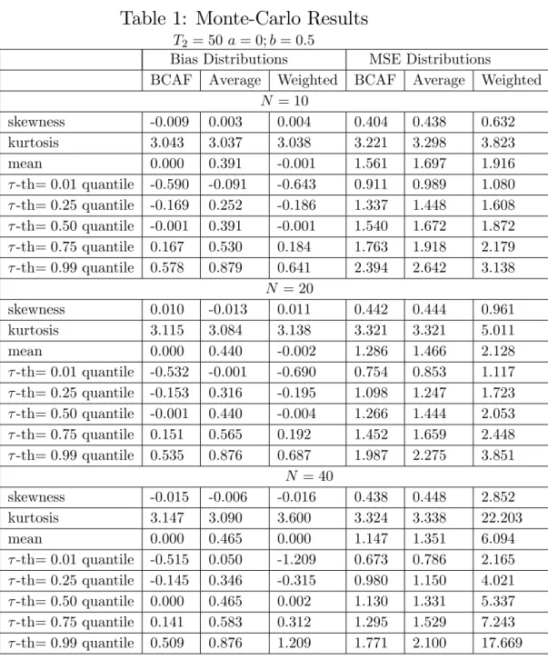
With the results of the 50;000 replications, we describe the empirical dis-tributions of the bias and the MSE of all three forecasting methods. For each distribution we compute the following statistics: (i) kurtosis; (ii) skew-ness, and (iii) -th unconditional quantile, with = 0:01;0:25;0:50;0:75; and 0:99. In doing so, we seek to have a general description of all three forecasting approaches.
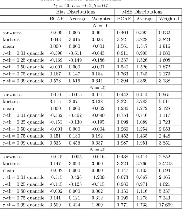
The main results are presented in Tables 1 and 2. In Table 1, B = 0:5, and, in Table 2, B = 0. In Table 1, the average bias across simulations of the BCAF and the weighted forecast combination are practically zero. The mean bias of the simple average forecast is between 0:39 and 0:46, depending onN. In terms of MSE, the BCAF performs very well compared to the other two methods. The simple average has a mean MSE at least
8:7%higher than that of the bias-corrected average forecast, reaching17:8%
higher whenN = 40. The weighted combination has an mean MSE at least
22:7% higher, reaching 431:3% higher when N = 40. This last result is a consequence of the increase in variance as we increaseN, withR…xed, and N=R close to unity. Notice that, when N = 40, N=R = 0:8. As stressed above, this results is expected if N=R is close to unity from below. Since R= 50, increasingN from10to40reveals the curse-of-dimensionality of the weighted forecast combination. For the other two methods, the distribution of MSE shrinks withN. For the BCAF, we reach an average MSE of1:147
whenN = 40, whereas the theoretical optimal MSE is1:000.
4
Empirical Application
4.1 The Central Bank of Brazil’s “Focus Forecast Survey”
The “Focus Forecast Survey,” collected by the Central Bank of Brazil, is a unique panel database of forecasts. It contains forecast information on al-most120institutions, including commercial banks, asset-management …rms, and non-…nancial institutions, which are followed throughout time with a reasonable turnover. Forecasts have been collected since1998, on a monthly frequency, and a …xed horizon, which potentially can serve to approximate a large N; T environment for techniques designed to deal with unbalanced panels – which is not the case studied here. Besides the large size ofN and T, the Focus Survey also has the following desirable features: the anonymity of forecasters is preserved, although the names of the top-…ve forecasters for a given economic variable is released by the Central Bank of Brazil; forecasts are collected at di¤erent frequencies (monthly, semi-annual, annual), as well as at di¤erent forecast horizons (e.g., short-run forecasts are obtained forh from 1 to 12 months); there is a large array of macroeconomic time series included in the survey.
To save space, we focus our analysis on the behavior of forecasts of the monthly in‡ation rate in Brazil ( t), in percentage points, as measured by
the o¢cial Consumer Price Index (CPI), computed by FIBGE. In order
to obtain the largest possible balanced panel (N T), we used N = 18
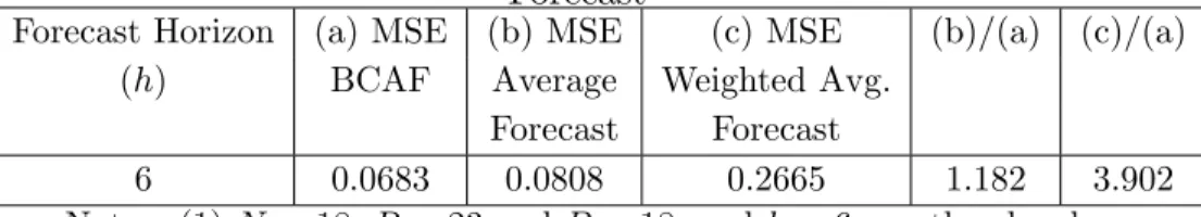
and a time-series sample period covering 2002:11 through 2006:3 (T = 41). Of course, in the case of a survey panel, there is no estimation sample. We chose the …rst R = 26 time observations to compute Bb – the average bias – leaving P = 18 time-series observations for out-of-sample forecast evaluation. The forecast horizon chosen wash= 6, this being an important horizon to determine future monetary policy within the Brazilian In‡ation-Targeting program.
4, out-of-sample forecast comparisons between the simple average and the bias-corrected average forecast show that the former has a MSE18:2% big-ger than that of the latter. We also computed the MSE of the weighted forecast. Since we have N = 18 and R = 26, N=R = 0:69. Hence, the weighted average cannot avoid the curse of dimensionality, yielding a MSE
390:2%bigger than that of the BCAF.
It is important to stress that, although the bias-corrected average fore-cast was conceived for a largeN; T environment, the empirical results here show an encouraging performance even in a smallN; T context. Also, the forecasting gains from bias correction are non-trivial.
5
Conclusions and Extensions
In this paper, we propose a novel approach to econometric forecast of station-ary and ergodic seriesyt within a panel-data framework, where the number
of forecasts and the number of time periods increase without bounds. The basis of our method is a two-way decomposition of the forecasts error. As shown here, this is equivalent to forecasters trying to approximate the op-timal forecast under quadratic loss – the conditional expectation Et h(yt),
which is modelled as the common feature of all individual forecasts. Stan-dard tools from panel-data asymptotic theory are used to devise an optimal forecasting combination that delivers Et h(yt). This optimal combination
uses equal weights and an estimated bias-correction term. The use of equal weights avoids estimating forecast weights, which contributes to reduce fore-cast variance, although potentially at the cost of an increase in bias. The use of an estimated bias-correction term eliminates any possible detrimental e¤ect arising from equal weighting. We label this optimal forecast as the (feasible)bias-corrected average forecast.
bias-correction term.
The Monte-Carlo experiment and the empirical analyses performed here show the usefulness of our new approach. In our Monte-Carlo simulations, when we considerN = 40, the simple average has a mean MSE17:8%higher than that of the feasible bias-corrected average forecast, while the weighted combination has a mean MSE 431:3%larger. In the empirical exercise, for N as low as18, the feasible bias-corrected average forecast leads to a sizable improvement in forecasting accuracy under MSE loss – from18% to about
390%– respectively regarding the simple and the weighted average.
As a by-product of the use of panel-data asymptotic methods, with N; T ! 1, we advanced the understanding of the forecast combination puz-zle. The key issue is that simple averaging requires no estimation of weights, while optimal weights requires estimating N weights that grow unbounded in the asymptotic setup. We show that there is no forecast-combination puzzle under certain asymptotic paths forN and T, but not for all. Indeed, ifN ! 1 at a rate strictly smaller than that of T, and lim
N;T!1N=T < 2,
then, the estimators of the weights are consistent, the weighted forecast with bias correction (intercept) is optimal, and there is no puzzle. Under di¤erent paths, it is impossible to obtain consistent estimators for the weights. For these paths, weights are not identi…ed, their estimates are unfeasible, and the variance of the weighted forecast diverges to in…nity. The Monte-carlo exercise illustrates a portion of such a path in …nite samples. There, the variance of the weighted forecast increases withN when R is …xed. IfN=R is close to unity from below, the variance component of the MSE of the weighted forecast will be large – larger, the closerN=R is to unity – and the simple average will be more accurate. This is the curse of dimensionality as an explanation to the puzzle.
References
[1] Amemiya, T. (1971), “The estimation of the variances in the variance-components model”,International Economic Review, vol. 12, pp. 1-13.
[3] Bai, J., (2005), “Panel Data Models with Interactive Fixed E¤ects,” Working Paper: New York University.
[4] Bai, J., and S. Ng, (2002), “Determining the Number of Factors in Approximate Factor Models,”Econometrica, 70, 191-221.
[5] Bates, J.M. and Granger, C.W.J., 1969, “The Combination of Fore-casts,” Operations Research Quarterly, vol. 20, pp. 309-325.
[6] Batchelor, R., 2007, “Bias in macroeconomic forecasts,” International Journal of Forecasting, vol. 23, pp. 189–203.
[7] Chamberlain, Gary, and Rothschild, Michael, (1983). “Arbitrage, Fac-tor Structure, and Mean-Variance Analysis on Large Asset Markets,”
Econometrica, vol. 51(5), pp. 1281-1304.
[8] Clark, T.E. and McCraken, M.W., 2007, “Combining Forecasts for Nested Models,” Working Paper: Kansas City FED, forthcoming in the Journal of Econometrics.
[9] Clements, M.P. and D.F. Hendry, 2006, Forecasting with Breaks in Data Processes, in C.W.J. Granger, G. Elliott and A. Timmermann (eds.)
Handbook of Economic Forecasting, pp. 605-657, Amsterdam, North-Holland.
[10] Conley, T.G., 1999, “GMM Estimation with Cross Sectional Depen-dence,”Journal of Econometrics, Vol. 92 Issue 1, pp. 1-45.
[11] Connor, G., and R. Korajzcyk (1986), “Performance Measurement with the Arbitrage Pricing Theory: A New Framework for Analysis,”Journal of Financial Economics, 15, 373-394.
[12] Davies, A. and Lahiri, K., 1995, “A new framework for analyzing survey forecasts using three-dimensional panel data,”Journal of Econometrics, vol. 68(1), pp. 205-227
[13] Elliott, G., C.W.J. Granger, and A. Timmermann, 2006, Editors, Hand-book of Economic Forecasting, Amsterdam: North-Holland.
[15] Elliott, G. and A. Timmermann (2004), “Optimal forecast combina-tions under general loss funccombina-tions and forecast error distribucombina-tions”,
Journal of Econometrics 122:47-79.
[16] Engle, R.F. (1982), “Autoregressive Conditional Heteroskedasticity with Estimates of the Variance of United Kingdom In‡ation,” Econo-metrica, 50, pp. 987-1006.
[17] Engle, R. F., Issler, J. V., 1995, “Estimating common sectoral cycles,”
Journal of Monetary Economics, vol. 35, 83–113.
[18] Engle, R.F. and Kozicki, S. (1993). “Testing for Common Features”,
Journal of Business and Economic Statistics, 11(4): 369-80.
[19] Forni, M., Hallim, M., Lippi, M. and Reichlin, L. (2000), “The Gener-alized Dynamic Factor Model: Identi…cation and Estimation”, Review of Economics and Statistics, 2000, vol. 82, issue 4, pp. 540-554.
[20] Forni M., Hallim M., Lippi M. and Reichlin L., 2003 “The Generalized Dynamic Factor Model one-sided estimation and forecasting,” Journal of the American Statistical Association, forthcoming.
[21] Fuller, Wayne A. and George E. Battese, 1974, “Estimation of linear models with crossed-error structure,” Journal of Econometrics, Vol. 2(1), pp. 67-78.
[22] Granger, C.W.J., 1989, “Combining Forecasts-Twenty Years Later,”
Journal of Forecasting, vol. 8, 3, pp. 167-173.
[23] Granger, C.W.J., and R. Ramanathan (1984), “Improved methods of combining forecasting”, Journal of Forecasting 3:197–204.
[24] Hendry, D.F. and M.P. Clements (2002), “Pooling of forecasts”, Econo-metrics Journal, 5:1-26.
[26] Issler, J. V., Vahid, F., 2001, “Common cycles and the importance of transitory shocks to macroeconomic aggregates,” Journal of Monetary Economics, vol. 47, 449–475.
[27] Issler, J. V., Vahid, F., 2006, “The missing link: Using the NBER reces-sion indicator to construct coincident and leading indices of economic
activity,” Annals Issue of the Journal of Econometrics on Common
Features, vol. 132(1), pp. 281-303.
[28] Kang, H. (1986), “Unstable Weights in the Combination of Forecasts,”
Management Science 32, 683-95.
[29] Laster, David, Paul Bennett and In Sun Geoum, 1999, “Rational Bias In Macroeconomic Forecasts,” The Quarterly Journal of Economics, vol. 114, issue 1, pp. 293-318
[30] Levin, A. and Lin, C.F. (1993), “Unit root tests in panel data: as-ymptotic and …nite-sample properties,” Discussion paper, University of California, San Diego.
[31] Palm, Franz C. and Arnold Zellner, 1992, “To combine or not to com-bine? issues of combining forecasts,” Journal of Forecasting, Volume 11, Issue 8 , pp. 687-701.
[32] Patton, Andrew J. and Allan Timmermann, 2006, “Testing Forecast Optimality under Unknown Loss,” forthcoming in the Journal of the American Statistical Association.
[33] Pesaran, M.H., (2005), “Estimation and Inference in Large Hetero-geneous Panels with a Multifactor Error Structure.” Working Paper: Cambridge University, forthcoming in Econometrica.
[34] Phillips, P.C.B. and H.R. Moon, 1999, “Linear Regression Limit Theory for Nonstationary Panel Data,” Econometrica, vol. 67 (5), pp. 1057– 1111.
[35] Quah, D. (1994), “Exploiting cross-section variation for unit root infer-ence in dynamic data,” Economics Letters, 44, pp. 9-19.
[37] Stock, J. and Watson, M., “Macroeconomic Forecasting Using Di¤usion Indexes”, Journal of Business and Economic Statistics, April 2002a, Vol. 20 No. 2, 147-162.
[38] Stock, J. and Watson, M., “Forecasting Using Principal Components from a Large Number of Predictors,” Journal of the American Statis-tical Association, 2002b.
[39] Stock, J. and Watson, M., 2006, “Forecasting with Many Predictors,”In: Elliott, G., C.W.J. Granger, and A. Timmermann, 2006, Editors, Hand-book of Economic Forecasting, Amsterdam: North-Holland, Chapter 10, pp. 515-554.
[40] Timmermann, A., 2006, “Forecast Combinations,” in Elliott, G.,
C.W.J. Granger, and A. Timmermann, 2006, Editors, Handbook of
Economic Forecasting, Amsterdam: North-Holland, Chapter 4, pp. 135-196.
[41] Vahid, F. and Engle, R. F., 1993, “Common trends and common cy-cles,” Journal of Applied Econometrics, vol. 8, 341–360.
[42] Vahid, F., Engle, R. F., 1997, “Codependent cycles,”Journal of Econo-metrics, vol. 80, 199–221.
[43] Vahid, F., Issler, J. V., 2002, “The importance of common cyclical fea-tures in VAR analysis: A Monte Carlo study,”Journal of Econometrics, 109, 341–363.
[44] Wallace, H. D., Hussain, A., 1969, “The use of error components model in combining cross-section and time-series data,”Econometrica, 37, 55– 72.
[45] West, K., 1996, “Asymptotic Inference about Predictive Ability,”
A
Tables and Figures
Table 1: Monte-Carlo Results
T2 = 50a= 0;b= 0:5
Bias Distributions MSE Distributions
BCAF Average Weighted BCAF Average Weighted
N = 10
skewness -0.009 0.003 0.004 0.404 0.438 0.632
kurtosis 3.043 3.037 3.038 3.221 3.298 3.823
mean 0.000 0.391 -0.001 1.561 1.697 1.916
-th= 0:01quantile -0.590 -0.091 -0.643 0.911 0.989 1.080
-th= 0:25quantile -0.169 0.252 -0.186 1.337 1.448 1.608
-th= 0:50quantile -0.001 0.391 -0.001 1.540 1.672 1.872
-th= 0:75quantile 0.167 0.530 0.184 1.763 1.918 2.179
-th= 0:99quantile 0.578 0.879 0.641 2.394 2.642 3.138
N = 20
skewness 0.010 -0.013 0.011 0.442 0.444 0.961
kurtosis 3.115 3.084 3.138 3.321 3.321 5.011
mean 0.000 0.440 -0.002 1.286 1.466 2.128
-th= 0:01quantile -0.532 -0.001 -0.690 0.754 0.853 1.117
-th= 0:25quantile -0.153 0.316 -0.195 1.098 1.247 1.723
-th= 0:50quantile -0.001 0.440 -0.004 1.266 1.444 2.053
-th= 0:75quantile 0.151 0.565 0.192 1.452 1.659 2.448
-th= 0:99quantile 0.535 0.876 0.687 1.987 2.275 3.851
N = 40
skewness -0.015 -0.006 -0.016 0.438 0.448 2.852
kurtosis 3.147 3.090 3.600 3.324 3.338 22.203
mean 0.000 0.465 0.000 1.147 1.351 6.094
-th= 0:01quantile -0.515 0.050 -1.209 0.673 0.786 2.165
-th= 0:25quantile -0.145 0.346 -0.315 0.980 1.150 4.021
-th= 0:50quantile 0.000 0.465 0.002 1.130 1.331 5.337
-th= 0:75quantile 0.141 0.583 0.312 1.295 1.529 7.243
Table 2: Monte-Carlo Results
T2 = 50; a= 0:5;b= 0:5
Bias Distributions MSE Distributions
BCAF Average Weighted BCAF Average Weighted
N = 10
skewness -0.009 0.005 0.004 0.404 0.395 0.632
kurtosis 3.043 3.016 3.038 3.221 3.228 3.823
mean 0.000 0.000 -0.001 1.561 1.547 1.916
-th= 0:01quantile -0.590 -0.511 -0.643 0.911 0.905 1.080
-th= 0:25quantile -0.169 -0.149 -0.186 1.337 1.326 1.608
-th= 0:50quantile -0.001 0.000 -0.001 1.540 1.526 1.872
-th= 0:75quantile 0.167 0.147 0.184 1.763 1.745 2.179
-th= 0:99quantile 0.578 0.516 0.641 2.394 2.369 3.138
N = 20
skewness 0.010 -0.015 0.011 0.442 0.414 0.961
kurtosis 3.115 3.071 3.138 3.321 3.283 5.011
mean 0.000 0.000 -0.002 1.286 1.272 2.128
-th= 0:01quantile -0.532 -0.462 -0.690 0.754 0.746 1.117
-th= 0:25quantile -0.153 -0.130 -0.195 1.098 1.089 1.723
-th= 0:50quantile -0.001 0.000 -0.004 1.266 1.254 2.053
-th= 0:75quantile 0.151 0.130 0.192 1.452 1.435 2.448
-th= 0:99quantile 0.535 0.456 0.687 1.987 1.951 3.851
N = 40
skewness -0.015 -0.005 -0.016 0.438 0.414 2.852
kurtosis 3.147 3.090 3.600 3.324 3.266 22.203
mean -0.002 0.000 0.000 1.147 1.133 6.094
-th= 0:01quantile -0.515 -0.426 -1.209 0.673 0.667 2.165
-th= 0:25quantile -0.145 -0.123 -0.315 0.980 0.971 4.021
-th= 0:50quantile -0.002 0.000 0.002 1.130 1.116 5.337
-th= 0:75quantile 0.141 0.121 0.312 1.295 1.278 7.243
Table 3:
The Brazilian Central Bank Focus Survey Computing Average Bias and Testing the No-Bias HypothesisHorizon (h) Avg. BiasBb H0 :B = 0
p-value
6 0:06187 0:063
Notes: (1)N = 18,R= 26,P = 15, and h= 6 months ahead.
Table 4:
The Brazilian Central Bank Focus SurveyComparing the MSE of Simple Average Forecast with that of the Bias-Corrected Average Forecast and the Weighted Average
Forecast
Forecast Horizon (a) MSE (b) MSE (c) MSE (b)/(a) (c)/(a)
(h) BCAF Average Weighted Avg.
Forecast Forecast
6 0:0683 0:0808 0:2665 1:182 3:902