No 668 ISSN 0104-8910
A Panel Data Approach to Economic
Forecasting: The Bias–Corrected Average
Forecast
Os artigos publicados são de inteira responsabilidade de seus autores. As opiniões
neles emitidas não exprimem, necessariamente, o ponto de vista da Fundação
A Panel Data Approach to Economic Forecasting:
The Bias-Corrected Average Forecast
João Victor Issler and Luiz Renato Limay Graduate School of Economics – EPGE
Getulio Vargas Foundation email: [email protected] and [email protected]
First Draft: December, 2006. This Version: February, 2008.
Abstract
In this paper, we propose a novel approach to econometric forecast-ing of stationary and ergodic time series within a panel-data frame-work. Our key element is to employ the (feasible) bias-corrected aver-age forecast. Using panel-data sequential asymptotics we show that it is potentially superior to other techniques in several contexts. In partic-ular, it is asymptotically equivalent to the conditional expectation, i.e., has an optimal limiting mean-squared error. We also develop a zero-mean test for the average bias and discuss the forecast-combination puzzle in small and large samples. Monte-Carlo simulations are con-ducted to evaluate the performance of the feasible bias-corrected aver-age forecast in …nite samples. An empirical exercise based upon data
We are especially grateful for the comments and suggestions given by two anonymous referees, Marcelo Fernandes, Wagner Gaglianone, Antonio Galvão, Ra¤aella Giacomini, Clive Granger, Roger Koenker, Marcelo Medeiros, Marcelo Moreira, Zhijie Xiao, and Hal White. We also bene…ted from comments given by the participants of the conference “Econometrics in Rio.” We thank Wagner Gaglianone and Claudia Rodrigues for excel-lent research assistance. João Victor Issler thanks the hospitality of the Rady School of Management, and the Department of Economics of UCSD, where parts of this paper were written. Both authors thank the hospitality of University of Illinois, where the …nal re-vision was written. João Victor Issler thanks the support of CNPq-Brazil, CAPES, and FAPERJ. Luiz Renato Lima thanks the support of CAPES. The usual disclaimer applies.
from a well known survey is also presented. Overall, theoretical and empirical results show promise for the feasible bias-corrected average forecast.
Keywords: Forecast Combination, Forecast-Combination Puzzle, Com-mon Features, Panel-Data, Bias-Corrected Average Forecast.
J.E.L. Codes: C32, C33, E21, E44, G12.
1
Introduction
Bates and Granger(1969) made the econometric profession aware of the ben-e…ts of forecast combination when a limited number of forecasts is consid-ered. The widespread use of di¤erent combination techniques has lead to an interesting puzzle from the econometrics point of view – the well known fore-cast combination puzzle: if we consider a …xed number of forecasts(N <1), combining them using equal weights(1=N) fare better than using “optimal weights” constructed to outperform any other forecast combination in the mean-squared error (MSE) sense.
Regardless of how one combines forecasts, if the series being forecast is stationary and ergodic, and there is enough diversi…cation among fore-casts, we should expect that a weak law-of-large-numbers (WLLN) applies to well-behaved forecast combinations. This argument was considered in Palm and Zellner (1992), who asked the question “to pool or not to pool” forecasts? Recently, Timmermann (2006) used risk diversi…cation – a prin-ciple so widespread in …nance – to defend pooling of forecasts. Of course, to obtain this WLLN result, at least the number of forecasts has to diverge
(N ! 1), which entails the use of asymptotic panel-data techniques. In our view, one reason that pooling forecasts has not yet been given a full asymp-totic treatment, with N; T ! 1, is that forecasting is frequently thought to be a time-series experiment, not a panel-data experiment.
of the conditional expectation of the series – the optimal forecast in the MSE sense. Indeed, the latter is thecommon feature of all individual fore-casts (Engle and Kozicki (1993)), while individual forefore-casts deviate from the optimal because of forecast misspeci…cation. Third, lettingN; T ! 1, we use standard tools from panel-data asymptotic theory to show that the pooling of forecasts delivers optimal limiting forecasts in the MSE sense. In our key result, we prove that, in the limit, the feasiblebias-corrected average forecast – equal weights in combining forecasts coupled with an estimated bias-correction term – is an optimal forecast identical to the conditional expectation.
The feasible bias-corrected average forecast is also parsimonious besides being optimal. The only parameter we need to estimate is the mean bias, for which we show consistency under the sequential asymptotic approach developed by Phillips and Moon (1999). Indeed, the only way we could increase parsimony in our framework is by doing without any bias correction. To test the usefulness of performing bias correction, we developed a zero-mean test for the average bias which draws upon the work of Conley (1999) on random …elds.
As a by-product of the use of panel-data asymptotic methods, with
N; T ! 1, we advance the understanding of the forecast combination puz-zle. The key issue is that simple averaging requires no estimation of weights, while optimal weights requires estimating N weights that grow unbounded in the asymptotic setup. We show that there is no puzzle under certain asymptotic paths forN andT, although that result does not hold generally. We are also able to discuss the puzzle in small samples, linking its presence to the curse of dimensionality which plagues so many estimators throughout econometrics1.
Despite the scarcity of panel-data studies on the pooling of forecasts2,
there has been panel-data research on forecasting focusing on the pooling of information; see Stock and Watson (1999 and 2002a and b) and Forni et al. (2000, 2003). Pooling forecasts is related to forecast combination
1We thank Roger Koenker for suggesting this asymptotic exercise to us, and an
anony-mous referee for casting the puzzle in terms of the curse of dimensionality.
2The notable exception is Palm and Zellner (1992), who discuss “to pool or not to
and operates a reduction on the space of forecasts. Pooling information operates a reduction on a set of highly correlated regressors. Forecasting can bene…t from the use of both procedures, since, in principle, both yield asymptotically optimal forecasts in the MSE sense.
A potential limitation in the literature on pooling of information is that pooling is performed in a linear setup, and the statistical techniques em-ployed were conceived as highly parametric – principal-component and fac-tor analysis. That is a problem if the conditional expectation is not a linear function of the conditioning set or if the parametric restrictions used (if any) are too stringent to …t the information being pooled. In this case, pooling forecasts will be a superior choice, since the forecasts being pooled need not be the result of estimating a linear model under a highly restric-tive parameterization. On the contrary, these models may be non-linear, non-parametric, and even unknown to the econometrician, as is the case of using a survey of forecasts. Moreover, the components of the two-way de-composition employed here are estimated using non-parametric techniques, dispensing with any distributional assumptions. This widens the application of the methods discussed in this paper.
Korajzcyk (1986), Phillips and Moon (1999), Bai and Ng (2002), Bai (2005), and Pesaran (2005). Indeed, our approach borrows from …nance the idea that we can only diversify idiosyncratic risk but not systematic risk. The lat-ter is associated with the common element of all forecasts – the conditional expectation term – which is to what a specially designed forecast average converges to.
The rest of the paper is divided as follows. Section 2 presents our main results and the assumptions needed to derive them. Section 3 presents the results of a Monte-Carlo experiment. Section 4 presents an empirical analy-sis using the methods proposed here, confronting the performance of our bias-corrected average forecast with that of other types of forecast combi-nation. Section 5 concludes.
2
Econometric Setup and Main Results
Suppose that we are interested in forecasting a weakly stationary and er-godic univariate process fytg using a large number of forecasts that will be combined to yield an optimal forecast in the mean-squared error (MSE) sense. These forecasts could be the result of using several econometric mod-els that need to be estimated prior to forecasting, or the result of using no formal econometric model at all, e.g., just the result of an opinion poll on the variable in question using a large number of individual responses. We can also imagine that some (or all) of these poll responses are generated using econometric models, but then the econometrician that observes these forecasts has no knowledge of them.
Regardless of whether forecasts are the result of a poll or of the esti-mation of an econometric model, we label forecasts of yt, computed using
conditioning sets lagged h periods, by fh
i;t, i = 1;2; : : : ; N. Therefore, fi;th
areh-step-ahead forecasts andN is either the number of models estimated to forecastyt or the number of respondents of an opinion poll regarding yt. We consider 3 consecutive distinct time sub-periods, where time is in-dexed byt= 1;2; : : : ; T1; : : : ; T2; : : : ; T. The …rst sub-periodEis labeled the “estimation sample,” where models are usually …tted to forecast yt in the subsequent period, if that is the case. The number of observations in it is
labeled the post-model-estimation or “training sample”, where realizations ofyt are usually confronted with forecasts produced in the estimation sam-ple, and weights and bias-correction terms are estimated, if need be. It has
R=T2 T1= 2 T observations in it, comprising (t=T1+ 1; : : : ; T2). The …nal sub-period isP (for prediction), where genuine out-of-sample forecast is entertained. It has P = T T2 = 3 T observations in it, comprising (t = T2 + 1; : : : ; T). Notice that 0 < 1; 2; 3 < 1, 1 + 2 + 3 = 1, and that the number of observations in these three sub-periods keep a …xed proportion with T – respectively, 1, 2 and 3 – being all O(T). This is an important ingredient in our asymptotic results forT ! 1.
We now compare our time setup with that of West. He only considers two consecutive periods: R data points are used to estimate models and the subsequentP data points are used for prediction. His setup does not require estimating bias-correction terms or combination weights, so there is no need for an additional sub-period for estimating the models that generate the
fh
i;t’s3. In the case of surveys, since we do not have to estimate models, our
setup is equivalent to West’s. Indeed, in his setup, R; P ! 1 asT ! 1, and lim
T!1R=P = 2[0;1]. Here 4:
lim
T!1
R
P =
2
3
= 2(0;1):
In our setup, we also let N go to in…nity, which raises the question of whether this is plausible. On the one hand, if forecasts are the result of estimating econometric models, they will di¤er across i if they are based either upon di¤erent conditioning sets or upon di¤erent functional forms of the conditioning set (or both). Since there is an in…nite number of func-tional forms that could be entertained for forecasting, this gives an in…nite number of possible forecasts. On the other hand, if forecasts are the result of a survey, although the number of responses is bounded from above, for all practical purposes, if a large enough number of responses is obtained, then the behavior of forecast combinations will be very close to the limiting behavior whenN ! 1.
3Notice that the estimated models generate the fh
i;t’s, but model estimation,
bias-correction estimation and weight estimation cannot be performed all within the same sub-sample in an out-of-sample forecasting exercise.
4To inlcude the endpoints of 2[0;1]we must give up either a training sample or a
Recall that, if we are interested in forecastingyt, stationary and ergodic, using information up toh periods prior to t, then, under a MSE risk func-tion, the optimal forecast is the conditional expectation using information available up to t h: Et h(yt). Using this well-known optimality result,
Hendry and Clements (2002) argue that the fact that the simple forecast
average N1
N
X
i=1
fh
i;t usually outperforms individual forecasts fi;th shows our
inability to approximate Et h(yt) reasonably well with individual models.
However, since Et h(yt) is optimal, this is exactly what these individual
models should be doing.
With this motivation, we write thefh
i;t’s as approximations to the optimal
forecast as follows:
fi;th =Et h(yt) +ki+"i;t, (1)
wherekiis the individual model time-invariant bias and"i;t is the individual model error term in approximatingEt h(yt), where E("i;t) = 0for alliand t. Here, the optimal forecast is a common feature of all individual forecasts and ki and "i;t arise because of forecast misspeci…cation5. We can always decompose the seriesyt intoEt h(yt) and an unforecastable component t,
such thatEt h( t) = 0 in:
yt=Et h(yt) + t. (2)
Combining (1) and (2) yields,
fi;th = yt t+ki+"i;t, or,
fi;th = yt+ki+ t+"i;t, where, t= t: (3)
Equation (3) is indeed the well known two-way decomposition, or error-component decomposition, of the forecast errorfh
i;t yt:
fi;th = yt+ i;t i= 1;2; : : : ; N; t > T1; (4)
i;t = ki+ t+"i;t.
5If an individual forecast is the conditional expectation
Et h(yt), thenki ="i;t = 0.
Notice that this implies that its MSE is smaller than that of 1
N N
X
i=1 fh
i;t, something that is
It has been largely used in econometrics dating back to Wallace and Hus-sein (1969), Amemiya (1971), Fuller and Battese (1974) and Baltagi (1980). Palm and Zellner (1992) employ a two-way decomposition to discuss fore-cast combination in a Bayesian and a non-Bayesian setup6, and Davies and Lahiri (1995) employed a three-way decomposition to investigate forecast rationality within the “Survey of Professional Forecasts.”
By construction, our framework in (4) speci…es explicit sources of fore-cast errors that are found in bothytandfi;th; see also the discussion in Palm
and Zellner and Davies and Lahiri. The termkiis the time-invariant forecast bias of modelior of respondenti. It captures the long-run e¤ect of forecast-bias of modeli, or, in the case of surveys, the time invariant bias introduced by respondent i. Its source is fh
i;t. The term t arises because forecasters
do not have future information on y between t h+ 1 and t. Hence, the source of t isyt, and it is an additive aggregate zero-mean shock a¤ecting
all forecasts equally7. The term"i;t captures all the remaining errors a¤ect-ing forecasts, such as those of idiosyncratic nature and others that a¤ect some but not all the forecasts (a group e¤ect). Its source isfi;th.
From equation (4), we conclude that ki; "i;t and t depend on the …xed horizon h. Here, however, to simplify notation, we do not make explicit this dependence on h. In our context, it makes sense to treat h as …xed and not as an additional dimension to i and t. In doing that, we follow West (1996) and the subsequent literature. As argued by Vahid and Issler (2002), forecasts are usually constructed for a few short horizons, since, as the horizon increases, the MSE in forecasting gets hopelessly large. Here,h
will not vary as much asiand t, especially becauseN; T ! 18.
6Palm and Zellner show that the performance of non-Bayesian combinations obey the
following MSE rank: (i) the unfeasible weighted forecast with known weights performs better or equal to the simple average forecast, and (ii) the simple average forecast may perform better than the feasible weighted forecast with estimated weights. Our main result is that the feasible bias-corrected average forecast is optimal under sequential asymptotics. We also propose an explanation to the forecast-combination puzzle based on the curse of dimensionality. Critical to these results is the use of largeN; T asymptotic theory.
7Because it is a component ofy
t, and the forecast error is de…ned asfi;th yt, the forecast
error arising from lack of future information should have a negative sign in (4); see (3). To eliminate this negative sign, we have de…ned tas the negative of this future-information
component.
8Davies and Lahiri considered a three-way decomposition withhas an added dimension.
From the perspective of combining forecasts, the componentski; "i;t and
tplay very di¤erent roles. If we regard the problem of forecast combination
as one aimed at diversifying risk, i.e., a …nance approach, then, on the one hand, the risk associated with "i;t can be diversi…ed, while that associated with t cannot. On the other hand, in principle, diversifying the risk asso-ciated with ki can only be achieved if a bias-correction term is introduced in the forecast combination, which reinforces its usefulness.
We now list our set of assumptions.
Assumption 1 We assume thatki; "i;tand tare independent of each other
for alliand t.
Independence is an algebraically convenient assumption used throughout the literature on two-way decompositions; see Wallace and Hussein (1969) and Fuller and Battese (1974) for example. At the cost of unnecessary complexity, it could be relaxed to orthogonality, something we avoid here.
Assumption 2 ki is an identically distributed random variable in the
cross-sectional dimension, but not necessarily independent, i.e.,
ki i.d.(B; 2k); (5)
where B and 2k are respectively the mean and variance of ki. In the time-series dimension, ki has no variation, therefore, it is a …xed parameter.
The idea of dependence is consistent with the fact that forecasters learn from each other by meeting, discussing, debating, etc. Through their ongo-ing interactions, they maintain a current collective understandongo-ing of where their target variable is most likely heading to, and of its upside and downside risks. Given the assumption of identical distribution forki,B represents the market (or collective) bias. Since we focus on combining forecasts, a pure idiosyncratic bias does not matter but a collective bias does. In principle, we
hbutkidoes not, the latter being critical to identifykiwithin their framework. Since, in
general, this restriction does not have to hold, our two-way decomposition is not nested into their three-way decompostion. Indeed, in our approach,ki varies with hand it is
could allow for heterogeneity in the distribution ofki – means and variances to di¤er acrossi. However, that will be a problem in testing the hypothesis that forecast combinations are biased.
It is desirable to discuss the nature of the term ki, which is related to the question of why we cannot focus solely on unbiased forecasts, for which
ki = 0. The role ofkiis to capture the long-run e¤ect, in the time dimension, of the bias of econometric models of yt, or of the bias of respondent i. We …rst discuss survey-based forecasts. In this case, a relevant question to ask is: why would forecasters introduce bias under an MSE risk function? Laster, Bennett and Geoum (1999), Patton and Timmermann (2006), and Batchelor (2007) list di¤erent arguments consistent with forecasters having a non-quadratic loss function. Following their discussion, we assume that all forecasters employ a combination of quadratic loss and a secondary loss function. Bias is simply a consequence of this secondary loss function and of the intensity in which the forecaster cares for it. The …rst example is that of a bank selling an investment fund. In this case, the bank’s forecast of the fund return may be upward-biased simply because it may use this forecast as a marketing strategy to attract new clients for that fund. Although the bank is penalized by deviating from Et h(yt), it also cares for selling the shares
of its fund. The second example introduces bias when there is a market forpessimism oroptimism in forecasting. Forecasters want to be labeled as optimists or pessimists in a “branding” strategy to be experts on “worst-” or on “best-case scenarios,“worst-” respectively. Batchelor lists governments as examples of experts on the latter.
In the case of model-based forecasts, bias results from model misspec-i…cation. Here, it is important to distinguish between in-sample and out-of-sample model …tting. The fact that, in sample, a model approximates well the data-generating process (DGP) of yt does not guarantee that it
or defective information set or incorrect model; and errors of measurement.
Assumption 3 The aggregate shock t is a stationary and ergodic M A
process of order at mosth 1, with zero mean and variance 2 <1.
Sincehis a bounded constant in our setup, tis the result of a cumulation
of shocks toyt that occurred betweent h+ 1and t. Being anM A( )is a consequence of the Wold representation forytand of (2). Ifyt is already an M A( )process of order smaller thanh 1, then its order will be the same as that of t. Otherwise, the order ish 1. In any case, it must be stressed that
tis unpredictable, i.e., thatEt h( t) = 0. This a consequence of (2) and of
the law of iterated expectations, simply showing that, from the perspective of the forecast horizonh, unless the forecaster has superior information, the aggregate shock t cannot be predicted.
Assumption 4: Let"t= ("1;t; "2;t; ::: "N;t)0 be a N 1 vector stacking the errors"i;t associated with all possible forecasts, where E("i;t) = 0 for alliandt. Then, the vector processf"tgis assumed to be
covariance-stationary and ergodic for the …rst and second moments, uniformly on
N. Further, de…ning i;t ="i;t Et 1("i;t), the innovation of "i;t, we
assume that
lim
N!1
1
N2
N
X
i=1
N
X
j=1
E i;t j;t = 0: (6)
Because the forecasts are computed h-steps ahead, forecast errors "i;t
can be serially correlated. Assuming that "i;t is weakly stationary is a way of controlling its time-series dependence. It does not rule out errors dis-playing conditional heteroskedasticity, since the latter can coexist with the assumption of weak stationarity; see Engle (1982).
Equation (6) limits the degree of cross-sectional dependence of the er-rors "i;t. It allows cross-correlation of the form present in a speci…c group of forecasts, although it requires that this cross-correlation will not pre-vent a weak law-of-large-numbers from holding. Following the forecasting literature with large N and T, e.g., Stock and Watson (2002b), and the …-nancial econometric literature, e.g., Chamberlain and Rothschild (1983), the condition lim
N!1
1
N2
PN
i=1
PN
j=1 E i;t j;t = 0 controls the degree of
that Chamberlain and Rothschild’s cross-sectional error dependence decay requires:
lim
N!1
1
N N
X
i=1
N
X
j=1
E i;t j;t <1: (7)
Notice that this is the same cross-sectional dependence decay used in Stock and Watson. Of course, (7) implies (6), but the converse is not true. Hence, Assumption 2 has a less restrictive condition than those commonly employed in the factor-model literature.
We state now basic results related to the classic question of “to pool or not to pool forecasts,” when only simple weights (1=N) are used; see, for example, Granger (1989) and Palm and Zellner (1992).
Proposition 1 Under Assumptions 1-4, the mean-squared error in
fore-castingyt, using the individual forecast fh
i;t, isE fi;th yt
2
=ki2+ 2+ 2i, where 2i is the variance of "i;t,i= 1;2; ; :::; N.
Proposition 2 Under Assumptions 1-4, as N ! 1, the mean-squared
er-ror in forecasting yt, combining all possible individual forecasts fi;th, is
M SEaverage =E plim
N!1
1
N N
X
i=1
fh
i;t yt
!2
=B2+ 2.
We can now compare the MSE of a generic individual forecast with that of an equally weighted(1=N) forecast combination by using the usual bias-variance standard decomposition of the mean squared error (MSE)
M SE=Bias2+V AR.
Proposition 1 shows that we can decompose individual MSE’s, M SEi, as:
M SEi = k2i + 2+ 2i
= Bias2i +V ARi,i= 1;2; :::; N
where Bias2i = k2i and V ARi = 2 + 2i. Proposition 2 shows that averaging forecasts reduces variance, but not necessarily MSE,
M SEaverage = B2+ 2 (8)
whereV ARaverage = 2 < V ARi = 2+ 2i, but comparing Bias2average =
B2 withBias2
i =ki2 requires knowledge of B and ki. IfB = 0, i.e., we are
considering unbiased forecasts, on average, thenM SEi =ki2+ 2+ 2i, while
M SEaverage = 2. Therefore, if the number of forecasts in the combination
is large enough, combining forecasts with a zero collective bias will lead to a smaller MSE – as concluded in Granger (1989). However, if B 6= 0, we cannot conclude that the average forecast has MSE lower than that of individual forecasts, sinceB2 may be larger or smaller than k2
i + 2i.
One way to eliminate the term B2 in (8) is to perform bias correction coupled with equal weights(1=N)in the forecast combination. The next set of results investigates the properties of the bias-corrected average forecast (BCAF).
Proposition 3 If Assumptions 1-4 hold, then, the bias-corrected average
forecast, given by N1
N
X
i=1
fh i;t N1
N
X
i=1
ki, obeys plim
N!1 1 N N X i=1 fh
i;t N1
N X i=1 ki ! =
yt+ t and has a mean-squared error as follows:
M SEBCAF = E
" plim N!1 1 N N X i=1 fh
i;t N1
N X i=1 ki ! yt #2
= 2. Therefore, it
is an optimal forecasting device in the MSE sense.
Proposition 3 shows that the bias-corrected average forecast is an optimal forecast in the MSE sense. Bias correction eliminates the termB2 from the MSE expression, while the use of equal weights naturally eliminates the variance of idiosyncratic components and group e¤ects. The only term left in the MSE is 2, related to unforecastable news to the target variable after the forecast combination was computed – something we could not eliminate unless we had superior (future) information. From a …nance perspective, all risks associated with terms that could be diversi…ed were eliminated by using the bias-corrected average forecast. We were left only with the undiversi…able risk expressed in 2. Therefore, the optimality result.
There are in…nite ways of combining forecasts. We now present an al-ternative weighting scheme to equal weights1=N.
Corollary 4 Consider the sequence of deterministic weights f!igNi=1, such
thatj!ij 6= 0; !i =O N 1 uniformly, and N
P
i=1
Then, under Assumptions 1-4,
plim
N!1
N
X
i=1
!ifi;th N
X
i=1
!iki yt
!
= t; and,
E
"
plim
N!1
N
X
i=1
!ifi;th N
X
i=1
!iki
!
yt
#2
= 2:
and the same result of Proposition 3 follows when a generic f!igNi=1 is used
instead of 1=N.
This corollary to Proposition 3 shows that there is not a unique optimum in the MSE sense. Indeed, any other combination scheme consistent with a WLLN will be optimal as well. Of course, optimal population weights, con-structed from the variance-covariance structure of models with stationary data, will obey the structure in Corollary 4. Hence, theoretically, optimal population weights cannot perform better than 1=N under bias correction. Therefore, there is no forecast-combination puzzle in the context of popula-tion weights.
Although the discussion using population weights is useful, the puzzle is associated with weights!i estimated using data. Then, the key question
to be answered analytically is why forecasts based on estimated weights are
not optimal. We now compare N1
N
X
i=1
fh
i;t with a bias-corrected version of
N
X
i=1
!ifh
i;t that uses estimated weights. We follow the discussion in Hendry
and Clements (2002) usingN di¤erent forecasts instead of just 2. Weights
!i can be estimated (!ib ) by running the following regression, minimizing
MSE subject to
N
X
i=1
!i = 1:
y= i+!1f1+!2f2+:::+!NfN+ , (9)
wherey denotes the R 1 vector of observations of the target variable, f1,
There are two cases to be considered: the behavior of estimated weights in small samples and asymptotically, when N; T ! 1. In large samples, consistent estimation of weights requires:
0< lim
N;T!1
N
R =N;Tlim!1
N=T T2 T1
T
= lim
N;T!1N=T
2
<1; (10)
which implies not only that N ! 1 at a smaller rate than T, but that
lim
N;T!1N=T < 2. Recall that 2 = 1 1 3, hence, N;Tlim!1N=T 1.
As long as this condition is achieved, weights are estimated consistently in (9) and we are back to Corollary 4: asymptotically, there is no forecast-combination puzzle. Notice that, because regression (9) includes an inter-cept, the forecast fb= bi+b!1f1 +!b2f2 +:::+!bNfN is unbiased with playing the role of a bias-correction term.
Because there is no puzzle asymptotically, the low accuracy of fb
rel-ative to that of N1
N
X
i=1
fh
i;t must re‡ect a poor small-sample
approxima-tion of populaapproxima-tion weights !is by the !ib s. In small samples, estimation of !i requires N < R. On the one hand, to get close to an optimal weighted forecast, we need a large N. On the other hand, the forecast
b
f =bi+!b1f1+!b2f2+:::+!Nb fN is not immune to the “curse of dimen-sionality,” since, asN increases, we need to estimate an increasing number of weights. Increasing N contributes to raising the variance of estimated weights, which works against the consistency of the!ib s.
As shown in our simulation exercise below, when N approachesR from below, the variance offbgrows withN and is typically big enough as to yield
an inferior forecast (MSE) relative to N1
N
X
i=1
fh
i;t, although the latter is biased.
Thus, the weighted forecast cannot avoid the “curse of dimensionality” that plagues several estimates across econometrics. In this context, the curse of dimensionality in fbis an explanation to the forecast-combination puzzle. Of course, if we make N=R close to zero in …nite samples, with N large, we allow!ib !p !i, sinceR will then be large. Moreover, the requirement of largeN guarantees the optimality result in Corollary 4.
MSE sense, but does not su¤er from the curse of dimensionality? Our answer to this question is the BCAF in Proposition 3. It borrows only the positive properties of …xed-weight(1=N) and estimated-weight forecasts. From the former, it inherits the fact that its variance decreases with N. From the latter, it inherits bias correction.
Despite its optimal behavior, it is immediately seen that the BCAF
1
N N
X
i=1
fi;th N1 N
X
i=1
ki is unfeasible since the ki’s are unknown. Therefore,
below, we propose replacingki with a consistent estimator. The underlying idea behind the consistent estimator ofkiis that one observes the realizations ofyt andfi;th,i= 1:::N, for theR training-sample observations. Hence, one
can form a panel of forecasts:
fi;th yt =ki+ t+"i;t; i= 1;2; : : : ; N; t=T1+ 1; ; T2; (11)
where it becomes obvious thatki represents the …xed e¤ect of this panel.
We propose a non-parametric estimator ofki. It does not depend on any distributional assumption onki i.d.(B; 2k)and it does not depend on any knowledge of the models used to compute the forecasts fh
i;t. This feature
of our approach widens its application to situations where the “underlying models are not known, as in a survey of forecasts,” as discussed by Kang (1986).
Due to the nature of our problem, which consists of a large number of forecasts and a time-invariant bias term(ki), we need to consider largeN, large T asymptotic theory to devise a consistent estimator for ki. Search-ing for a method that allows robust asymptotic results without imposSearch-ing too many restrictions (on functional relations and the existence of higher moments), we consider the sequential asymptotic approach developed by Phillips and Moon (1999). There, one …rst …xes N and then allows T to pass to in…nity using an intermediate limit. Phillips and Moon write sequen-tial limits of this type as (T; N ! 1)seq. We now show how to estimate consistentlyki,B, t, and "i;t, in this context.
esti-mators of ki, B, t, and"i;t, respectively:
b
ki = 1
R
PT2
t=T1+1fi;th
1
R
PT2
t=T1+1yt, plim
T!1
b
ki ki = 0,
b
B = 1
N
PN
i=1bki, plim
(T;N!1)seq
b
B B = 0,
bt =
1
N N
X
i=1
fi;th Bb yt, plim
(T;N!1)seq
(bt t) = 0,
b"i;t = fi;th yt bki bt, plim
(T;N!1)seq
(b"i;t "i;t) = 0:
We now state our most important result.
Proposition 6 If Assumptions 1-4 hold, the feasible bias-corrected
aver-age forecast N1
N
X
i=1
fi;th Bb obeys plim
(T;N!1)seq 1
N N
X
i=1
fi;th Bb
!
= yt+ t =
Et h(yt) and has a mean-squared error as follows:
E
"
plim
(T;N!1)seq 1 N N X i=1 fh
i;t Bb
!
yt
#2
= 2. Therefore it is an optimal
forecasting device.
Proposition 6 shows that the feasible BCAF is asymptotically equivalent to the optimal weighted forecast. Its advantage is that it employs equal weights. AsN ! 1, the number of estimated parameters is kept at unity:
b
B. This is a very attractive feature of the BCAF compared to devices that combine forecasts using estimated weights. Our answer to the curse of dimensionality is parsimony, implied by estimating only one parameter –
b
B. Here, we need not limit the asymptotic path of N; T as is the case of forecasts based on estimated weights.
We must stress that bias-correction can be viewed as a form of intercept correction as discussed in Palm and Zellner (1992) and Hendry and Mizon (2005), for example. From (9), we could retrieveBb from an OLS regression of the form:
y= i+!1f1+!2f2+:::+!NfN+ ,
terms of the previous literature9.
Finally, we propose a new test for the usefulness of bias correction (H0 :
B= 0) using the theory of random …elds as in Conley (1999). It is potentially relevant when we viewBas amarketor aconsensusbias, which is customary in the …nance and macroeconomics literature, respectively. When B = 0,
the feasible BCAF becomes N1
N
X
i=1
fh i;t.
Proposition 7 Under the null hypothesis H0:B = 0, the test statistic:
b
t= pBb b
V
d
!
(T;N!1)seqN (0;1);
whereVb is a consistent estimator of the asymptotic variance ofB = N1
N
X
i=1
ki.
2.1 The BCAF and Nested Models
It is important to discuss whether and when the techniques above are ap-plicable to the situation where some (or all) of the models we combine are nested. The potential problem is that the innovations from nested mod-els can exhibit high cross-sectional dependence, violating Assumption 4. In what follows, we introduce nested models into our framework in the follow-ing way. Consider a continuous set of models and split the total number of modelsN into M classes (or blocks), each of them containing m nested models, so thatN =mM. In the index of forecasts, i= 1; ::; N, we group nested models contiguously. Hence, models within each class are nested but models across classes are non-nested. We make the number of classes and the number of models within each class to be functions of N, respectively as follows: M = N1 d and m = Nd, where 0 d 1. Notice that this
setup considers all the relevant cases: (i) d= 0 corresponds to the case in which all models are non-nested; (ii)d= 1corresponds to the case in which all models are nested and; (iii) the intermediate case0< d <1gives rise to
N1 d blocks of nested models, all with sizeNd.
9Recall thatBb requires estimating only onebk
i separately using R observations. For
For each block of nested models, Assumption 4 may not hold because the innovations from that block can exhibit high cross-sectional dependence10.
Regarding the interaction across blocks of nested models, it is natural to impose that the correlation structure of innovations across classes is such that Assumption 4 holds, since we should expect that the cross-sectional dependence of forecast errors across classes is weak. We formalize this by using the following extension to equation (6) in Assumption 4.
Assumption 5: Consider the covariance matrix of innovations, given by
E i;t j;t , and partition it into blocks. There areM main-diagonal
blocks, each withm2 =N2delements. These blocks contain the
covari-ance structure of innovations for each class of nested models. There are alsoM2 M o¤-diagonal blocks which represents the across-block covariance structure of innovations. Index the classes (blocks) of mod-els byr= 1; ::; M, and models within each class (block) bys= 1; ::; m. For allt, and anyr and s, we may re-index r;s;t to (r 1)m+s;t = i;t, i= 1; :::; N11. Within each blockr, we assume that:
0 lim m!1 1 m2 m X k=1 m X s=1
E r;k;t r;s;t = lim
N!1
1
N2d Nd X k=1 Nd X s=1
E r;k;t r;s;t <1;
(12) being zero when the smallest nested model is correctly speci…ed. How-ever, across any two blocks r and l,r6=l, we assume that:
lim m!1 1 m2 m X k=1 m X s=1
E r;k;t l;s;t = lim
N!1
1
N2d
Nd X k=1 Nd X s=1
E r;k;t l;s;t = 0:
(13)
We now discuss how to implement the BCAF in the presence of nested models. The matrix E i;t j;t has N2 = m2M2 elements, but only m2M = N2dN1 d =N1+d represent covariances among nested models, in
which condition (12) holds. For the remaining elements, (13) holds. Unless
d= 1, the total number of elements representing covariances among nested
1 0As discussed in great detail below, Assumption 4 will hold for nested models if the
smallest nested model is correctly speci…ed.
1 1For example,
models (N1+d) will grow at a rate smaller than N2 – the total number of elements. Therefore, Assumption 4 will still hold in the presence of nested models when0< d <1, and our result on optimality of the BCAF will still follow. Notice that0< d < 1 corresponds to the case in which nested and non-nested models are combined and the number of nested models grows withN.
We now consider two special cases: if d= 0, there are only non-nested models, since each class of models has only one element. Hence, Assumption 4 holds. Ifd= 1, we only have one class of models, and all models are nested. In general, Assumption 4 will not hold, and a law-of-large numbers will not apply to N1 PNi=1"i;t. We now discuss in detail the special case in which d= 1and the smallest model is correctly speci…ed. It is easy to verify that, for the smallest model, the following equation will hold withki ="i;t = 0in population:
fi;th =Et h(yt) +ki+"i;t. (14)
This happens because, under correct speci…cation of the smallest model in the nesting scheme, its population forecast will be Et h(yt), making ki ="i;t= 0. This, in turn, makes i;t ="i;t Et 1("i;t) = 0for the smallest model. When the smallest nesting model is correctly speci…ed, all models that nest it will have identical population errors, i.e., will haveki ="i;t = 0
as well. This happens because any model that nests the smallest one will have irrelevant estimated parameters that will converge to zero, in proba-bility. Therefore, condition (12) will hold as an equality, and a law-of-large numbers will apply to N1 PNi=1"i;t as a degenerate case, where there is no variation in population, among the elements being combined.
From an empirical point of view, dcan be regarded as a choice variable when implementing the BCAF. Choosing d = 1 (only one class of nested models) is an “excellent” choice when the class of model chosen is correctly speci…ed (the smallest model is correctly speci…ed). However, there is the (potentially high) risk of incorrect speci…cation for the whole class, which will imply that the law-of-large numbers will not hold for N1 PNi=1"i;t in im-plementing the BCAF. On the other hand, in choosingd= 0(all models are non-nested), we completely eliminate nested models and the chance that the law-of-large numbers will not hold. In the intermediate case,0< d <1, we have nested models but can still apply a law-of-large numbers for N1 PNi=1"i;t
poses no problem at all, since the mixture of models will still deliver the op-timal forecast. From a practical point of view, the choice of0 d <1seems to be superior. Here, we are back to the main theorem in …nance about risk diversi…cation: do not put all your eggs in the same basket, choosing a large enough number of diversi…ed (classes of) models.
3
Monte-Carlo Study
3.1 Experiment design
We follow the setup presented in the theoretical part of this paper in which each forecast is the conditional expectation of the target variable plus an ad-ditive bias term and an idiosyncratic error. Our DGP is a simple stationary
AR(1)process:
yt = 0+ 1yt 1+ t,t= 1; :::T1; :::; T2; :::; T (15)
t i.i.d.N(0;1), 0 = 0, and 1= 0:5,
where t is an unpredictable aggregate zero-mean shock. We focus on one-step-ahead forecasts for simplicity. The conditional expectation of yt is Et 1(yt) = 0 + 1yt 1. Since t is unpredictable, the forecaster should
be held accountable for fi;t Et 1(yt). These deviations have two terms: the individual speci…c biases (ki) and the idiosyncratic or group error terms ("i;t). Because t i.i.d.N(0;1), the optimal theoretical MSE is unity in this
exercise.
The conditional expectation Et 1(yt) = 0+ 1yt 1 is estimated using a sample of size 200, i.e., E =T1 = 200, so that b0 ' 0 and b1 ' 1: In practice, however, forecasters may have economic incentives to make biased forecasts, and there may be other sources of misspeci…cation arising from misspeci…cation errors. Therefore, we generate forecasts as:
fi;t = b0+b1yt 1+ki+"i;t; (16)
= (b0+ki) +b1yt 1+"i;t for t=T1+ 1; ; T,i= 1; :::N;
where, ki = ki 1 +ui, ui i.i.d.Uniform(a; b), 0 < < 1, and "t =
distribution of"i;t. The diagonal elements of = ( ij)obey: 1< ii<
p
10, and o¤-diagonal elements obey: ij = 0:5, if ji jj = 1, ij = 0:25, if
ji jj = 2, and ij = 0, if ji jj > 2. The exact values of the ii’s
are randomly determined through an once-and-for-all draw from a uniform random variable of sizeN, that is, ii i.i.d.Uniform(1;
p
10)12.
In equation (16), we built spatial dependence in the bias termki13. The cross-sectional average of ki is 2(1a+b). We set the degree of spatial depen-dence inki by letting = 0:5. For the support ofui, we consider two cases:
(i) a= 0 and b= 0:5 and; (ii)a= 0:5 and b= 0:5. This implies that the average bias isB = 0:5in (i), whereas it isB = 0in (ii). Finally, notice that the speci…cation of"i;tsatis…es Assumption 4 in Section 2 as we letN ! 1.
Equation (16) is used to generate di¤erent panels of forecasts in terms of the number of forecasters (N) and the size of the training-sample (R). We kept the number of out-of-sample observations equal toP = 50in all cases. First, for N = 10;20;40, we let R = 50. For all these 3 cases, NR may not be small enough to guarantee a good approximation of optimal population weights by the !ib s. In order to approximate the asymptotic environment needed for optimality of the forecasts based on estimated weights, i.e., equa-tion (10), we also considered the case in which R = 500, and 1;000, while keepingN = 10. For eachN, we conducted50;000simulations in the exper-iment. In all cases, the total number of time observations used to …t models equalsE =T1= 200.
3.2 Forecast approaches
In our simulations, we evaluate three forecasting methods: the feasible bias-corrected average forecast (BCAF), the forecast based on estimated weights, and the forecast based on …xed weights. For these methods, our results include aspects of the whole distribution of their respective biases and MSEs. For the BCAF, we use the training-sample observations to estimatebki =
1 2The covariance matrix does not change over simulations. 1 3The additive bias k
i is explicit in (16). It could be implicit if we had considered
a structural break in the target variable as did Hendry and Clements (2002). There, an intercept change in yt takes place right after the estimation of econometric models,
1
R T2
P
t=T1+1
(yt fi;t) and Bb = N1
N
P
i=1
b
ki. Then, we compute the out-of-sample
forecastsfbBCAF
t = N1
N
P
i=1
fi;t Bb,t=T2+ 1; :::; T, and we employ the last
P observations to compute M SEBCAF = P1 T
P
t=T2+1
yt fbBCAF
t
2 .
For the forecast based on estimated weights (weighted average forecast), we use R observations of the training sample to estimate weights (!i) by OLS in:
y= i+!1f1+!2f2+:::+!NfN+",
where the restriction
N
X
i=1
!i = 1 is imposed in estimation. The weighted
forecast is fbtweighted =b+b!1f1;t+!b2f2;t+:::+b!NfN;t, and the intercept
plays the role of bias correction. We employ the last P observations to
computeM SEweighted = P1
T
P
t=T2+1
yt fbtweighted 2.
For the forecast based on …xed weights (average forecast), there is no pa-rameter to be estimated using training-sample observations. Out-of-sample
forecasts are computed according to ftaverage = N1
N
P
i=1
fi;t, t=T2+ 1; :::; T,
and its MSE is computed asM SEaverage= P1
T
P
t=T2+1
(yt ftaverage)2.
Finally, for each approach, we also computed the out-of-sample mean biases. In small samples, the weighted forecast and the BCAF should have out-of-sample mean biases close to zero, whereas the mean bias of the average forecast should be close to B= a+b
2(1 ).
3.3 Simulation Results
With the results of the50;000replications, we describe the empirical distrib-utions of the bias and the MSE of all three forecasting methods. For each dis-tribution we compute the following statistics: (i) kurtosis; (ii) skewness, (iii) mean and (iv) -th unconditional quantile, with = 0:01;0:25;0:50;0:75;
and 0:99. In doing so, we seek to have a general description of all three forecasting approaches.
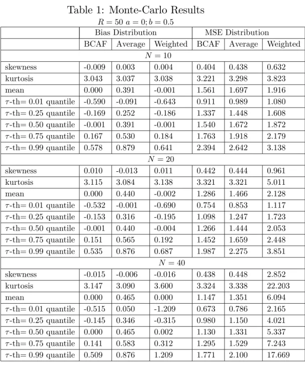
The main results are presented in Tables 1 through 4. In Table 1, where
forecast are practically zero. The mean bias of the simple average fore-cast is between 0:39 and 0:46, depending on N. In terms of MSE, the BCAF performs very well compared to the other two methods. The sim-ple average forecast has a mean MSE at least8:7%higher than that of the bias-corrected average forecast, reaching17:8%higher whenN = 4014. The
forecast based on estimated weights has a mean MSE at least22:7%higher, reaching431:3% higher when N = 40. This last result is a consequence of the increase in variance as we increaseN, with R …xed, and N=R close to unity. Notice that the average bias is virtually zero forN = 10;20;40. Since the MSE triples whenN is increased from10to40, all the increase in MSE is due to variance, revealing the curse-of-dimensionality working against the forecast based on estimated weights.
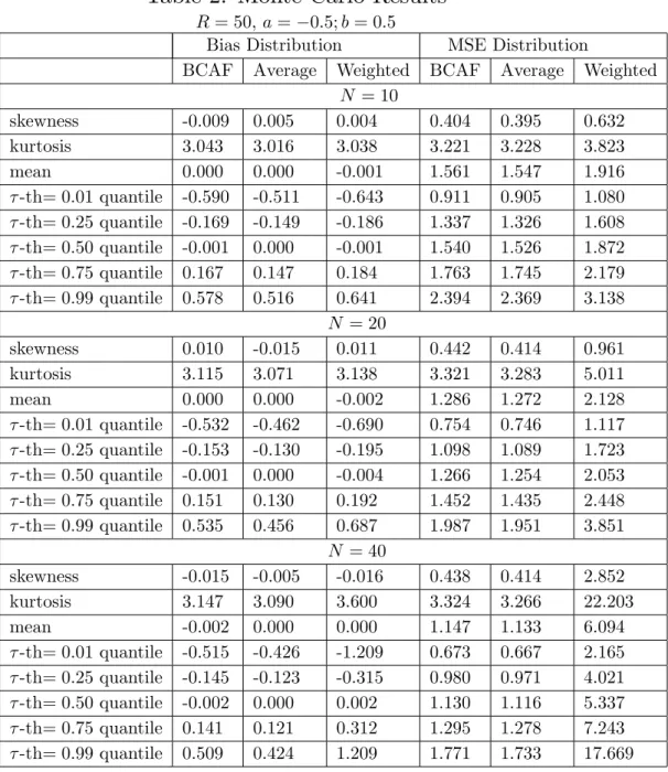
Table 2 presents the results when B = 0. In this case, the optimal forecast is the simple average, since there is no need to estimate a bias-correction term. In terms of MSE, comparing the simple-average forecast with the BCAF, we observe that they are almost identical – the mean MSE of the BCAF is about1%higher than that of the average forecast, showing that not much is lost in terms of MSE when we perform an unnecessary bias correction. The behavior of the weighted average forecast is identical to that in Table 1.
Table 3 presents the result in which B = 0:5, NR 0, andN = 10, with
R= 500;1;000. As expected, the!bis are a very good approximation to
opti-mal population weights. Despite that, we are still combining a relatively low number of forecasts: N = 10. Here, there is practically no di¤erence in per-formance between the BCAF and the estimated-weight forecast. However, contrary to the results in Tables 1 and 2, equal-weight forecasts perform worse than estimated-weight forecasts. Indeed, the MSE of the simple av-erage is at least 8:9% higher than that of the estimated-weight forecast, while the latter has an almost identical accuracy to the BCAF: no bias, and a variance (and MSE) that is more than 50% than that of the theoretical optimum 2 = 1.
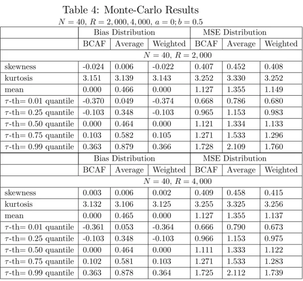
Table 4 presents the result in which B = 0:5, NR 0, andN = 40, with
R= 2;000;4;000. Although the ratio N
R was kept identical to that in Table
1 4When we compare the MSE of the …xed-weight forecast with that of the optimal
forecast (which is unity in our simulation), we observe that the former converges towards
3, we have now increased bothN and R proportionally. As in Table 3, the
b
!is are a very good approximation to optimal population weights, sinceR
is large. However, contrary to the results there, now we are also combining an increasing number of forecasts: 40 vs. 10. As a result, not only BCAF and the estimated-weight forecast outperform the …xed-weight forecast, but they also are closer to the theoretical optimum 2 = 1 (about 15% worse here as opposed to more than 50%in Table3).
One key insight from the results in Tables 1-4 is that no combination device outperforms the BCAF by a wide margin, and, even when the BCAF is not constructed to be optimal – Table 2 – its performance is practically identical to that of the optimal forecast.
4
Empirical Application
4.1 The Central Bank of Brazil’s “Focus Forecast Survey”
The “Focus Forecast Survey,” collected by the Central Bank of Brazil, is a unique panel database of forecasts. It contains forecast information on al-most120institutions, including commercial banks, asset-management …rms, and non-…nancial institutions, which are followed throughout time with a reasonable turnover. Forecasts have been collected since1998, on a monthly frequency, and a …xed horizon, which potentially can serve to approximate a large N; T environment for techniques designed to deal with unbalanced panels – which is not the case studied here. Besides the large size ofN andT, the Focus Survey also has the following desirable features: the anonymity of forecasters is preserved, although the names of the top-…ve forecasters for a given economic variable are released by the Central Bank of Brazil; forecasts are collected at di¤erent frequencies (monthly, semi-annually, annually), as well as at di¤erent forecast horizons (e.g., short-run forecasts are obtained for h from 1 to 12 months); there is a large array of macroeconomic time series included in the survey.
To save space, we focus our analysis on the behavior of forecasts of the monthly in‡ation rate in Brazil ( t), in percentage points, as measured by
the o¢cial Consumer Price Index (CPI), computed by FIBGE. In order to obtain the largest possible balanced panel (N T), we used N = 18
Of course, in the case of a survey panel, there is no estimation sample. We chose the …rst R = 26 time observations to compute Bb – the average bias – leaving P = 18 time-series observations for out-of-sample forecast evaluation. The forecast horizon chosen wash= 6, this being an important horizon to determine future monetary policy within the Brazilian In‡ation-Targeting program.
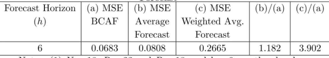
The results of our empirical exercise are presented in Tables 5 and 6. First, we note that all the 18 individual forecasts perform worse than com-binations, which is consistent with the discussion in Hendry and Clements (2002). The results in Table 5 show that the average bias is positive for the 6-month horizon,0:06187, and marginally signi…cant, with a p-value of0:063. This is a sizable bias – approximately0:75percentage points in a yearly ba-sis, for an average in‡ation rate of5:27%a year. In Table 6, out-of-sample forecast comparisons between the simple average and the bias-corrected av-erage forecast show that the former has a MSE 18:2% bigger than that of the latter. We also computed the MSE of the weighted forecast. Since we haveN = 18andR= 26,N=R= 0:69. Hence, the weighted average cannot avoid the curse of dimensionality, yielding an MSE390:2%bigger than that of the BCAF.
It is important to stress that, although the feasible BCAF was conceived for a largeN; T environment, the empirical results here show an encouraging performance even in a small N; T context. Also, the forecasting gains from bias correction are non-trivial.
5
Conclusions and Extensions
In this paper, we propose a novel approach to the econometric forecast of stationary and ergodic series yt within a panel-data framework, where the number of forecasts and the number of time periods increase without bound. The basis of our method is a two-way decomposition of forecast errors. As shown here, this is equivalent to forecasters trying to approximate the op-timal forecast under quadratic loss – the conditional expectation Et h(yt),
which is modelled as the common feature of all individual forecasts. Stan-dard tools from panel-data asymptotic theory are used to devise an optimal forecasting combination that delivers Et h(yt). This optimal combination
weights avoids estimating forecast weights, which contributes to the reduc-tion of forecast variance, although potentially at the cost of an increase in bias. The use of an estimated bias-correction term eliminates any possi-ble detrimental e¤ect arising from equal weighting. We label this optimal forecast as the (feasible)bias-corrected average forecast.
We show that the feasible BCAF delivers the optimality result even under the presence of nested models and we fully characterize it by using a novel framework. As a by-product of the use of panel-data asymptotic methods, with N; T ! 1, we advance the understanding of the forecast combination puzzle by showing that the low accuracy of the forecasts based on estimated weights, relative to those based on …xed weights, re‡ects a poor small-sample approximation of optimal population weights!is by estimated weights. In small samples, estimation of !i requires N < R. On the one hand, to get close to an optimal weighted forecast, we need a largeN. On the other hand, the forecast based on estimated weights is not immune to the “curse of dimensionality,” since, as N increases, we need to estimate an increasing number of weights. In our simulations, we show that the curse of dimensionality works against forecasts based on estimated weights, increasing their MSE asN approaches R.
Finally, we show that there is no forecast-combination puzzle under cer-tain asymptotic paths forN and T, but not in all cases. Indeed, ifN ! 1
at a rate strictly smaller than T, then !i is consistently estimated, the
weighted forecast with bias correction (intercept) is optimal, and there is no puzzle. Our simulations approximate this asymptotic environment by considering various cases in which N=T 0. As expected, the forecast based on estimated weights outperforms the simple …xed-weight combina-tion and has the same performance as the BCAF. Since the case in which
N=T 0is rarely observed in practice, we should not expect forecasts based on estimated-weight combinations to be accurate. On the other hand, the feasible BCAF is asymptotically equivalent to the optimal-weight forecast but has a superior performance in small samples.
References
[2] Baltagi, Badi H., 1980, “On Seemingly Unrelated Regressions with Er-ror Components,” Econometrica, Vol. 48(6), pp. 1547-1551.
[3] Bai, J., (2005), “Panel Data Models with Interactive Fixed E¤ects,” Working Paper: New York University.
[4] Bai, J., and S. Ng, (2002), “Determining the Number of Factors in Approximate Factor Models,”Econometrica, 70, 191-221.
[5] Bates, J.M. and Granger, C.W.J., 1969, “The Combination of Fore-casts,” Operations Research Quarterly, vol. 20, pp. 309-325.
[6] Batchelor, R., 2007, “Bias in macroeconomic forecasts,” International Journal of Forecasting, vol. 23, pp. 189–203.
[7] Chamberlain, Gary, and Rothschild, Michael, (1983). “Arbitrage, Fac-tor Structure, and Mean-Variance Analysis on Large Asset Markets,”
Econometrica, vol. 51(5), pp. 1281-1304.
[8] Clark, T.E. and McCracken, M.W., 2007, “Combining Forecasts for Nested Models,” Working Paper: Kansas City FED, forthcoming in the Journal of Econometrics.
[9] Clements, M.P. and Hendry, D.F. (1996), “Intercept Corrections and Structural Change”, Journal of Applied Econometrics , vol. 11, pp. 475-494.
[10] Clements, M.P. and D.F. Hendry, 2006, Forecasting with Breaks in Data Processes, in C.W.J. Granger, G. Elliott and A. Timmermann (eds.)
Handbook of Economic Forecasting, pp. 605-657, Amsterdam, North-Holland.
[11] Conley, T.G., 1999, “GMM Estimation with Cross Sectional Depen-dence,”Journal of Econometrics, Vol. 92 Issue 1, pp. 1-45.
[12] Connor, G., and R. Korajzcyk (1986), “Performance Measurement with the Arbitrage Pricing Theory: A New Framework for Analysis,”Journal of Financial Economics, 15, 373-394.
[14] Elliott, G., C.W.J. Granger, and A. Timmermann, 2006, Editors, Hand-book of Economic Forecasting, Amsterdam: North-Holland.
[15] Elliott, G. and A. Timmermann (2005), “Optimal forecast combina-tion weights under regime switching”, International Economic Review, 46(4), 1081-1102.
[16] Elliott, G. and A. Timmermann (2004), “Optimal forecast combina-tions under general loss funccombina-tions and forecast error distribucombina-tions”,
Journal of Econometrics 122:47-79.
[17] Engle, R.F. (1982), “Autoregressive Conditional Heteroskedasticity with Estimates of the Variance of United Kingdom In‡ation,” Econo-metrica, 50, pp. 987-1006.
[18] Engle, R. F., Issler, J. V., 1995, “Estimating common sectoral cycles,”
Journal of Monetary Economics, vol. 35, 83–113.
[19] Engle, R.F. and Kozicki, S. (1993). “Testing for Common Features”,
Journal of Business and Economic Statistics, 11(4): 369-80.
[20] Forni, M., Hallim, M., Lippi, M. and Reichlin, L. (2000), “The Gener-alized Dynamic Factor Model: Identi…cation and Estimation”, Review of Economics and Statistics, 2000, vol. 82, issue 4, pp. 540-554.
[21] Forni M., Hallim M., Lippi M. and Reichlin L., 2003 “The Generalized Dynamic Factor Model one-sided estimation and forecasting,” Journal of the American Statistical Association, forthcoming.
[22] Fuller, Wayne A. and George E. Battese, 1974, “Estimation of linear models with crossed-error structure,” Journal of Econometrics, Vol. 2(1), pp. 67-78.
[23] Granger, C.W.J., 1989, “Combining Forecasts-Twenty Years Later,”
Journal of Forecasting, vol. 8, 3, pp. 167-173.
[24] Granger, C.W.J., and R. Ramanathan (1984), “Improved methods of combining forecasting”, Journal of Forecasting 3:197–204.
[26] Hendry, D.F. and Mizon, G.E. (2005): “Forecasting in the Presence of Structural Breaks and Policy Regime Shifts”, in “Identi…cation and Inference for Econometric Models: Essays in Honor of Thomas Rothen-berg,” D.W.K. Andrews and J.H. Stock (eds.), Cambridge University Press.
[27] Issler, J. V., Vahid, F., 2001, “Common cycles and the importance of transitory shocks to macroeconomic aggregates,” Journal of Monetary Economics, vol. 47, 449–475.
[28] Issler, J. V., Vahid, F., 2006, “The missing link: Using the NBER reces-sion indicator to construct coincident and leading indices of economic activity,” Annals Issue of the Journal of Econometrics on Common Features, vol. 132(1), pp. 281-303.
[29] Kang, H. (1986), “Unstable Weights in the Combination of Forecasts,”
Management Science 32, 683-95.
[30] Laster, David, Paul Bennett and In Sun Geoum, 1999, “Rational Bias In Macroeconomic Forecasts,” The Quarterly Journal of Economics, vol. 114, issue 1, pp. 293-318
[31] Palm, Franz C. and Arnold Zellner, 1992, “To combine or not to com-bine? issues of combining forecasts,” Journal of Forecasting, Volume 11, Issue 8 , pp. 687-701.
[32] Patton, Andrew J. and Allan Timmermann, 2006, “Testing Forecast Optimality under Unknown Loss,” forthcoming in the Journal of the American Statistical Association.
[33] Pesaran, M.H., (2005), “Estimation and Inference in Large Hetero-geneous Panels with a Multifactor Error Structure.” Working Paper: Cambridge University, forthcoming in Econometrica.
[34] Phillips, P.C.B. and H.R. Moon, 1999, “Linear Regression Limit Theory for Nonstationary Panel Data,” Econometrica, vol. 67 (5), pp. 1057– 1111.
[36] Stock, J. and Watson, M., “Macroeconomic Forecasting Using Di¤usion Indexes”, Journal of Business and Economic Statistics, April 2002a, Vol. 20 No. 2, 147-162.
[37] Stock, J. and Watson, M., “Forecasting Using Principal Components from a Large Number of Predictors,” Journal of the American Statis-tical Association, 2002b.
[38] Stock, J. and Watson, M., 2006, “Forecasting with Many Predictors,”In: Elliott, G., C.W.J. Granger, and A. Timmermann, 2006, Editors, Hand-book of Economic Forecasting, Amsterdam: North-Holland, Chapter 10, pp. 515-554.
[39] Timmermann, A., 2006, “Forecast Combinations,” in Elliott, G., C.W.J. Granger, and A. Timmermann, 2006, Editors, Handbook of Economic Forecasting, Amsterdam: North-Holland, Chapter 4, pp. 135-196.
[40] Vahid, F. and Engle, R. F., 1993, “Common trends and common cy-cles,” Journal of Applied Econometrics, vol. 8, 341–360.
[41] Vahid, F., Engle, R. F., 1997, “Codependent cycles,”Journal of Econo-metrics, vol. 80, 199–221.
[42] Vahid, F., Issler, J. V., 2002, “The importance of common cyclical fea-tures in VAR analysis: A Monte Carlo study,”Journal of Econometrics, 109, 341–363.
[43] Wallace, H. D., Hussain, A., 1969, “The use of error components model in combining cross-section and time-series data,”Econometrica, 37, 55– 72.
[44] West, K., 1996, “Asymptotic Inference about Predictive Ability,”
Econometrica, 64, (5), pp. 1067-84.
A
Appendix
A.1 Proofs of Propositions in Section 2
Proof of Proposition 1:. Start with:
Then, the MSE of individual forecasts is:
M SEi = E fi;th yt
2
=E(ki+ t+"i;t)2 (17)
= E k2i +E 2t +E "2i;t
= ki2+ 2+ 2i;
where 2
i is the variance of "i;t. Assumption 1 is used in the second line of
(17). We also use the fact thatki is a constant in the time-series dimension in the last line of (17).
Proof of Proposition 2:. Start with the cross-sectional average of (4):
1
N N
X
i=1
fi;th yt=
1
N N
X
i=1
ki+ t+
1
N N
X
i=1
"i;t.
Computing the probability limit of the right-hand side above gives,
plim N!1 1 N N X i=1
ki+ t+ plim
N!1 1 N N X i=1 "i;t: (18)
We will compute the probability limits in (18) separately. The …rst one is a straightforward application of the law of large numbers:
plim N!1 1 N N X i=1
ki=B.
The second will turn out to be zero. Our strategy is to show that, in
the limit, the variance of N1
N
X
i=1
"i;t is zero, a su¢cient condition for a weak
law-of-large-numbers to hold forf"i;tgNi=1.
Because"i;t is weakly stationary and mean-zero, for everyi, there exists
a scalar Wold representation of the form:
"i;t= 1 X
j=0
bi;j i;t j (19)
where, for alli,bi;0= 1,Pj1=0b2i;j <1, and i;t is white noise.
In computing the variance of N1
N X i=1 1 X j=0
bi;j i;t j we use the fact that
we need only to consider the sum of the variances of terms of the form 1
N
PN
i=1bi;k i;t k. These variances are given by:
VAR 1
N N
X
i=1
bi;k i;t k
! = 1 N2 N X i=1 N X j=1
bi;kbj;kE i;t j;t ; (20)
due to weak stationarity of "t. We now examine the limit of the generic term in (20) with detail:
VAR 1
N N
X
i=1
bi;k i;t k
! = 1 N2 N X i=1 N X j=1
bi;kbj;kE i;t j;t
1 N2 N X i=1 N X j=1
bi;kbj;kE i;t j;t =
1 N2 N X i=1 N X j=1
jbi;kbj;kj E i;t j;t (21)
max
i;j jbi;kbj;kj
1 N2 N X i=1 N X j=1
E i;t j;t :
(22)
Hence:
lim
N!1VAR
1
N N
X
i=1
bi;k i;t k
!
lim
N!1 maxi;j jbi;kbj;kj
lim N!1 1 N2 N X i=1 N X j=1
E i;t j;t = 0;
since the sequencefbi;jg1j=0is square-summable, yielding lim
N!1 maxi;j jbi;kbj;kj <
1, and Assumption 4 imposes lim
N!1 1 N2 PN i=1 PN
j=1 E i;t j;t = 0.
Thus, all variances are zero in the limit, as well as their sum, which gives:
plim N!1 1 N N X i=1
"i;t = 0:
Therefore, E plim N!1 1 N N X i=1
fi;th yt
!2
= E(B+ t)2
Proof of Proposition 3:. From the proof of Proposition 2, we have: plim N!1 1 N N X i=1
fi;th yt plim
N!1 1 N N X i=1
ki = t+ plim
N!1 1 N N X i=1 "i;t
= t;
leading to: E " plim N!1 1 N N X i=1
fi;th 1 N N X i=1 ki ! yt #2
= 2:
Proof of Proposition 5:. Although yt; t and "i;t are ergodic for the mean, fh
i;t is non ergodic because of ki. Recall that, T1; T2; R ! 1, as
T ! 1. Then, as T ! 1,
1
R
PT2
t=T1+1f
h
i;t =
1
R
PT2
t=T1+1yt+
1
R
PT2
t=T1+1"i;t+
1
R
PT2
t=T1+1 t+ki
p
!E(yt) +ki+E("i;t) +E( t)
= E(yt) +ki
Given that we observe fh
i;t and yt, we propose the following consistent
esti-mator forki, asT ! 1:
b
ki =
1
R
PT2
t=T1+1f
h i;t
1
R
PT2
t=T1+1yt, i= 1; :::; N
= 1
R
PT2
t=T1+1(yt+ki+ t+"i;t)
1
R
PT2
t=T1+1yt
= ki+ 1
R
PT2
t=T1+1"i;t+
1
R
PT2
t=T1+1 t or,
b
ki ki = 1
R
PT2
t=T1+1"i;t+
1
R
PT2
t=T1+1 t:
Using this last result, we can now propose a consistent estimator for B:
b
B = 1
N
PN
i=1bki=
1 N PN i=1 1 R
PT2
t=T1+1fi;th
1
R
PT2
t=T1+1yt .
First let T ! 1,
b
ki !p ki, and,
1 N N X i=1 b ki p ! 1 N N X i=1
Now, as N ! 1, after T ! 1, 1 N N X i=1
ki!p B;
Hence, as (T; N ! 1)seq,
plim (T;N!1)seq
b
B B = 0:
We can now propose a consistent estimator for t:
bt=
1
N N
X
i=1
fi;th Bb yt= 1
N N
X
i=1
fi;th 1 N
N
X
i=1
b
ki yt.
We let T ! 1 to obtain:
plim T!1 1 N N X i=1
fi;th 1 N N X i=1 b ki yt ! = 1 N N X i=1
fi;th 1 N
N
X
i=1
ki yt
= t+ 1
N N
X
i=1
"i;t:
Letting now N ! 1, we obtain plim
N!1 1 N N X i=1
"i;t = 0and:
plim (T;N!1)seq
(bt t) = 0:
Finally,
b"i;t = fi;th yt bki bt, andfi;th yt=ki+ t+"i;t. Hence :
b
"i;t "i;t = ki bki + ( t bt):
Using the previous results that plim
T!1
b
ki ki = 0and plim
(T;N!1)seq
(bt t) =
0, we obtain:
plim (T;N!1)seq