www.ann-geophys.net/28/75/2010/
© Author(s) 2010. This work is distributed under the Creative Commons Attribution 3.0 License.
Annales
Geophysicae
The Empirical Forcing Function as a tool for the diagnosis of
large-scale atmospheric anomalies
C. Andrade1,2, J. A. Santos3, J. G. Pinto4, J. Corte-Real2, and S. Leite3 1Polytechnic Institute of Tomar, Portugal
2ICAAM: Group Water, Soil and Climate, University of ´Evora, Portugal 3CITAB, University of Tr´as-os-Montes e Alto Douro, Portugal
4Institute for Geophysics and Meteorology, University of Cologne, Germany
Received: 8 May 2009 – Revised: 4 January 2010 – Accepted: 6 January 2010 – Published: 15 January 2010
Abstract. The time-mean quasi-geostrophic potential vor-ticity equation of the atmospheric flow on isobaric surfaces can explicitly include an atmospheric (internal) forcing term of the stationary-eddy flow. In fact, neglecting some non-linear terms in this equation, this forcing can be mathemat-ically expressed as a single function, called Empirical Forc-ing Function (EFF), which is equal to the material derivative of the time-mean potential vorticity. Furthermore, the EFF can be decomposed as a sum of seven components, each one representing a forcing mechanism of different nature. These mechanisms include diabatic components associated with the radiative forcing, latent heat release and frictional dissipation, and components related to transient eddy trans-ports of heat and momentum. All these factors quantify the role of the transient eddies in forcing the atmospheric circu-lation. In order to assess the relevance of the EFF in diagnos-ing large-scale anomalies in the atmospheric circulation, the relationship between the EFF and the occurrence of strong North Atlantic ridges over the Eastern North Atlantic is an-alyzed, which are often precursors of severe droughts over Western Iberia. For such events, the EFF pattern depicts a clear dipolar structure over the North Atlantic; cyclonic (an-ticyclonic) forcing of potential vorticity is found upstream (downstream) of the anomalously strong ridges. Results also show that the most significant components are related to the diabatic processes. Lastly, these results highlight the rele-vance of the EFF in diagnosing large-scale anomalies, also providing some insight into their interaction with different physical mechanisms.
Keywords. Meteorology and atmospheric dynamics (Cli-matology; General circulation; Synoptic-scale meteorol-ogy)
Correspondence to:C. Andrade ([email protected])
1 Introduction
The temporal mean flow of the atmosphere can be regarded as a forced regime that is conditioned by several factors, e.g., heat release, topography and surface thermal contrasts (Wal-lace and Hobbs, 2006). However, eddies embedded in the time-mean flow induce local transient heat and momentum fluxes that are key forcing mechanisms of the general atmo-spheric circulation. In fact, such eddies are essential for ex-plaining the energy cycle of the atmosphere, as they contin-uously transform zonal-mean available potential energy into eddy and zonal-mean kinetic energy of the flow that is ul-timately dissipated through cascading frictional dissipation processes (e.g., Peixoto and Oort, 1992). The key role played by the eddy transports concerning the maintenance of large-scale atmospheric anomalies through their interaction with the zonal-mean flow has been already demonstrated in many previous studies (e.g., Edmon et al., 1980; Holopainen et al., 1982; Hoskins and Valdes, 1990; Lau and Nath, 1991; Black, 1998; Santos et al., 2009b).
Vorticity is a widely used property when describing the dy-namical characteristics of the flow, and its equation is com-monly used for diagnosis and prediction of fluid motions (Hoskins et al., 1985; Holton, 2004). Potential vorticity is a quantity that combines vorticity and static stability and ver-ifies an invertibility principle that can be stated as follows (Bluestein, 1993): if the distribution of potential vorticity is known, then vorticity, static stability and wind field can also be determined, providing the required boundary conditions and a condition. The concept of potential vorticity is often used in the study of the atmospheric circulation, particularly when considering an adiabatic frictionless flow (Salby and Roger, 1996); in this case it is materially conserved (local rate of change is entirely balanced by advection). Therefore, potential vorticity is commonly written in its original formu-lation on isentropic surfaces (Ertel, 1942). However, many
subsequent studies have also used the potential vorticity de-fined on isobaric surfaces (e.g., Hartmann, 1977; Lau and Wallace, 1979). In fact, potential vorticity is also materially conserved when using the quasi-geostrophic formulation of the potential vorticity under the quasi-geostrophic assump-tions and following the geostrophic wind on an isobaric sur-face (Holton, 2004).
The mathematical formulation of the quasi-geostrophic potential vorticity equation in isobaric coordinates is revis-ited in the present study. Some mathematical approxima-tions and rearrangements are undertaken so as to obtain a lin-earized version of the equation, where various forcing terms are explicitly and independently represented. The forcing term of the stationary-eddy (asymmetric) potential vortic-ity is expressed as a single function, called the Empirical Forcing Function (hereafter EFF). This function can be in turn decomposed as a sum of seven components that repre-sent different physical contributions (associated with diabatic processes and transient eddy enthalpy and momentum trans-ports) to the total forcing term of the balance equation. This development closely follows the original formulation under-taken by Saltzman (1962).
In order to illustrate the applicability of the EFF in diag-nosing large-scale atmospheric anomalies, a case study fo-cusing on the establishment of ridges over the Eastern North Atlantic is presented. Previous studies have shown that the frequency and persistence of such events are often associ-ated with droughts over western Iberia (Santos et al., 2007a). Here, precipitation is characterized by a strong seasonal be-haviour reaching a maximum during the winter season (De-cember to February; hereafter DJF). As a result, extremely wet or extremely dry winters tend to have strong impacts on water availability and management practices (Garc´ıa-Herrera et al., 2007). Due to this vulnerability, with great environ-mental, economical and social significance, it is of great importance to better understand the large-scale mechanisms that are linked to the occurrence of such droughts.
The influence of these enhanced ridges over the Eastern North Atlantic in the mid-latitude weather systems is also tested here. In fact, these systems have their origin in pro-cesses predicted under the theory of baroclinic instability and their development is closely associated with the above referred forcing mechanisms. Such extra-tropical migratory systems follow a path in the belt of the prevailing westerly winds and derive their existence and growth from the conver-sion of available potential energy to kinetic energy by dimin-ishing the temperature gradients, lifting mid-latitude warm air and sinking cold polar air (Charney, 1947; Eady, 1949). They also play a central role in the angular momentum bud-get of the atmosphere and are primarily responsible for main-taining the westerlies against surface friction (Peixoto and Oort, 1992). One common measure of synoptic activity is the “storm track”, which Blackmon (1976) defined as the stan-dard deviation of the bandpass-filtered (2–6 days) variability at 500 hPa. This variable has been widely used to quantify
synoptic activity, both for observational and model data sets (e.g., Hoskins and Valdes, 1990; Stephenson and Held, 1993; Chang and Fu, 2002; Yin, 2005; Ulbrich et al., 2008; Chang, 2009).
In this study, the objectives are then two-fold. First, it is intended to present the mathematical development of the EFF, and secondly, to demonstrate its relevance in diagnos-ing large-scale anomaly patterns by considerdiagnos-ing a pertinent case study. The structure of this text is as follows: Sect. 2 presents the mathematical formulation of the EFF; Sect. 3 describes data and methodologies; Sect. 4 presents the re-sults obtained for the selected case study and, lastly, Sect. 5 discusses the main results of this study.
2 Mathematical development of the Empirical Forcing Function
2.1 Fundamental equations and Empirical Forcing Function deduction
The mathematical development of the EFF involves funda-mental equations and definitions and was first presented by Saltzman (1962). The following notation is used in the de-velopment; () represents the time-mean, ()′ time-mean de-parture,hirepresents the zonal-mean (average taken over a parallel) and()∗the zonal-mean departure. Considering the time-mean primitive equations of motion in spherical coordi-nates, after Reynolds decomposition ω=ω+ω′, the zonal
momentum equation can be written as
∂u
∂t +v• ∇u+ω ∂u ∂p=
f+utanϕ a
v− 1 acosϕ
∂8
∂λ +X (1)
and the meridional momentum equation as
∂v
∂t +v• ∇v+ω ∂v ∂p= −
f+utanϕ a
u−1 a
∂8
∂ϕ +Y (2)
where variablesXandY can be defined as
X=Fλ−
"
1
acosϕ ∂u′2
∂λ +
1
acosϕ ∂ ∂ϕu
′v′cosϕ
+∂u ′ω′ ∂p −
u′v′tanϕ a
#
(3)
Y =Fϕ−
"
1
acosϕ ∂v′u′
∂λ +
1
acosϕ ∂ ∂ϕv
′2cosϕ
+∂v ′ω′ ∂p +
u′2tanϕ
a
#
(4) The time-mean energy equation, also after Reynolds decom-position, can be written as follows
∂T
∂t +v• ∇T+ω ∂T
∂p = R pcp
ωT+Q (5)
where variableQcan be defined as
Q=q˙F+ ˙qR+ ˙qL cp
−
"
1
acosϕ ∂u′T′
∂λ +
1
acosϕ ∂ ∂ϕv
′T′cosϕ
+∂ω ′T′ ∂p −
R pcp
ω′T′
#
(6) In the previous equation,q˙R,q˙F andq˙Lare the rates of heat addition per unit mass due to radiation, conduction and fric-tion and latent heat release, respectively.
Now consider the continuity equation
∂ω
∂p+ ∇ •v=0, (7)
the hydrostatic equation
∂8 ∂p = −
RT
p , (8)
and the stability parameter
Ŵ=T θ ∂θ ∂p= ∂T ∂p− RT pcp , (9)
which is considered constant at each isobaric level (Saltz-man, 1962; Savij¨arvi, 1978). Finally, consider the quasi-geostrophic potential vorticity definition (Savij¨arvi, 1978; Holton, 2004),5,
5=η+f ∂ ∂p T Ŵ (10) whereη=ζ+f is the absolute vorticity,ζ the relative vor-ticity,f =2cosϕ the planetary vorticity andf∂p∂ TŴthe stretching vorticity (Holton, 2004).
From the quasi-geostrophic potential vorticity definition, after applying the local time-derivative, the next relation is obtained ∂5 ∂t = ∂η ∂t + ∂ ∂t f ∂ ∂p T Ŵ (11) as well as the following vector decomposition
v• ∇5=v• ∇η+v• ∇
f ∂ ∂p T Ŵ . (12)
Adding to the vorticity equation
∂η
∂t+v• ∇η+ω ∂η
∂p+η∇ •v+k∇ω× ∂v
∂p−k• ∇×F=0, (13)
the terms ∂t∂
f∂p∂ TŴ+v• ∇f∂p∂ TŴ, the following equation is obtained
∂η ∂t
|{z}
(11)
+v• ∇η
| {z }
(12)
+ω∂η∂p+η∇ •v+k∇ω×∂v
∂p−k• ∇ ×F
+∂ ∂t f ∂ ∂p T Ŵ
| {z }
(11)
+v• ∇
f ∂ ∂p T Ŵ
| {z }
(12)
=∂t∂ f∂p∂ TŴ+v• ∇f ∂ ∂p
T Ŵ
(14)
After some mathematical developments (for further details see Appendix A) and taking the time-mean, the time-mean potential vorticity equation is then attained
∂5
∂t +v• ∇5=2+ζ ∂ω ∂p−ω
∂ζ
∂p−k∇ω× ∂v ∂p +∂ ∂p T Ŵ !
v• ∇f−f Ŵ
∂v ∂p• ∇T
+f T Ŵ2
∂v
∂p• ∇Ŵ−f ∂ ∂p
T
Ŵ2 v• ∇Ŵ
! −f ∂ ∂p T Ŵ2 ∂Ŵ ∂t ! (15)
where2is defined as
2=f ∂ ∂p
Q Ŵ
!
+k• ∇ ×F
=f ∂ ∂p
Q Ŵ
!
+ 1
acosϕ ∂Y ∂λ−
∂Xcosϕ ∂ϕ
!
. (16)
In Eq. (16),Qis the sum of the diabatic heating terms related to transient temperature fluxes, whereasXandY are the sum of the frictional dissipative components with the terms re-lated to transient momentum fluxes.
Noting that the second member of Eq. (15) is the sum of
2with non-linear terms, as follows
∂5
∂t +v• ∇5=2+non-linear terms. (17)
Now considering only the stationary-eddy (asymmetric) components in Eq. (15) and neglecting all non-linear asym-metric terms, the equation of the stationary-eddy potential vorticity is obtained
∂5∗
∂t ≈ − v• ∇5
∗ +f ∂ ∂p Q Ŵ !∗ + 1
acosϕ ∂Y ∂λ−
∂ ∂ϕXcosϕ
!∗
∂5∗
∂t ≈ − v• ∇5
∗
+2∗≈0 (18)
According to Saltzman (1962), this approximation is reason-able when means are taken over a sufficiently long time pe-riod, such as an entire season. In this case, the term2∗can be interpreted as a forcing term of the stationary-eddy poten-tial vorticity and is also called EFF. Since the local derivative of the stationary-eddy potential vorticity also tends to be ne-glected when considering an entire season (steady-state), the EFF tends to be balanced by advection, i.e., the advection pattern tends to be in phase opposition with the EFF pattern. Having in mind this EFF definition, it should be stressed that
its analysis is essentially a diagnostic tool, not enabling stud-ies of the development of the anomalstud-ies (onset/decay).
It is still worth emphasizing that the external forcing mech-anisms of the atmospheric circulation (boundary conditions), such as topographic effects, diabatic fluxes at the lower at-mospheric boundary are not incorporated in this definition. In fact, only internal (mechanical and thermal) processes are taken into consideration in the EFF formulation. Since these internal processes interact through positive and nega-tive feedback mechanisms with the mean flow, they cannot be considered as independent forcing entities of the atmospheric flow. For instance, positive eddy feedback mechanisms have been shown to play a key role in the reinforcement of tele-connection patterns, such as the North Atlantic Oscillation (Rivi`ere, 2009).
2.2 EFF components
In order to separate the contributions of different processes to the total forcing, the EFF can be expressed as a sum of seven additive components,
2∗=
7
X
n=1
ffn(λ,ϕ,p). (19)
Therefore, regions of positive (negative) values offfn repre-sent a cyclonic (anticyclonic) forcing of the stationary-eddy potential vorticity. It should be noted the possibility that large scale potential vorticity anomalies set up without be-ing caused by any underlybe-ing forcbe-ing mechanism; in such case, under steady conditions, those anomalies will not be advected by the atmospheric flow, with the consequence that they would remain undetected by the present analysis. This possibility deserves further investigation, which falls outside the scope of this paper. In the present work it is assumed that the onset of circulations resulting in dry or wet winters in continental Portugal is due to forcing effects which reflect on different patterns of the empirical forcing function.
Substituting Eqs. (3), (4) and (6) in (16) and taking the zonal-mean departure, the component separation of the EFF is attained. The mathematical formulation of each compo-nent is as follows:
ff1=f
∂ ∂p
1
Ŵ ˙ qR+ ˙qF
cp
!!∗
(20)
is associated with friction and diabatic heating,
ff2=f
∂ ∂p 1 Ŵ ˙ qL cp !!∗ (21)
is associated with latent heat release,
ff3= −f
∂ ∂p
1
Ŵ ∂u′T′
∂λ + ∂ ∂ϕv
′T′cosϕ
!!∗
(22)
is related to the differential divergence of the transient-eddy horizontal transports of enthalpy,
ff4= −f
∂ ∂p
1
Ŵ
∂ω′T′ ∂λ −
R pcp
ω′T′
!!
(23)
is associated with the differential divergence of the vertical transient-eddy transports of enthalpy,
ff5= k• ∇ ×F
∗
(24) is linked to friction,
ff6= − 1
a2cosϕ
1 cosϕ
∂ ∂λ
∂u′v′ ∂λ +
∂ ∂ϕv
′2cosϕ+u′2sinϕ
!
− ∂ ∂ϕ
∂u′2 ∂λ +
∂ ∂ϕu
′v′cosϕ−u′v′sinϕ
!#∗
(25)
is associated with the transient horizontal transports of mo-mentum,
ff7= − 1
acosϕ ∂ ∂p
∂v′ω′ ∂λ −
∂ ∂ϕu
′ω′cosϕ
!∗
(26)
is related to the transient vertical transports of momentum. For the second component, the rate of heat addition per unit mass due to condensation,q˙L, was calculated indirectly from the water vapour continuity equation,
˙ qL= −L
∂q
∂t +v• ∇q+ω ∂q ∂p ! = −L ∂q
∂t +v• ∇q+ ∂ωq
∂p
≈ −L
∇ •vq+∂ωq ∂p
˙
qL≈ −L 1
acosϕ ∂uq
∂λ +
1
acosϕ ∂
∂ϕvqcosϕ+
1
acosϕ ∂u′q′
∂λ
+ 1
acosϕ ∂ ∂ϕv
′q′cosϕ+∂ωq ∂p +
∂ω′q′ ∂p
!
(27)
For the first component, the sum of the rates of heat addi-tion per unit mass due to radiaaddi-tion and due to conducaddi-tion and frictionq˙R+ ˙qF, respectively, were indirectly computed from the energy conservation Eqs. (5) and (27), following a similar development. As such,
˙
qL+ ˙qR+ ˙qF ≈cp 1
acosϕ ∂uT
∂λ +
1
acosϕ ∂
∂ϕvTcosϕ
+ 1
acosϕ ∂u′T′
∂λ +
1
acosϕ ∂ ∂ϕv
′T′cosϕ
+∂ωT ∂p +
∂ω′T′ ∂p −
R pcp
ωT− R pcp
ω′T′
!
(28)
Consequently,
˙
qR+ ˙qF= ˙qL+ ˙qR+ ˙qF− ˙qL. (29) It is worth mentioning that due to the impossibility of obtain-ing the fifth component, related to frictional effects, the EFF considered here is the sum of the remaining six components.
3 Data and methodology
The NCEP/NCAR reanalysis dataset (Kistler et al., 2001) de-fined on a 2.5◦×2.5◦grid is used. Only data up to 250 hPa is considered in the present study. Daily means for the period 1957–2008 are computed from 6-hourly data. Climate-mean values refer to averages calculated using the standard refer-ence period from 1961 to 1990 (WMO, 1996). Since the ap-plication of the EFF is based on the fundamental assumption that the atmospheric properties (e.g., transient transports) are averaged over a relatively long time period, the time-means in all equations presented in the previous section refer to an entire winter period (DJF). The corresponding departures are then computed on a daily basis after seasonal correction (de-partures relative to the mean calendar day). Although the computations were performed for the entire Northern Hemi-sphere, as winter-mean ridges over the Eastern North At-lantic are the selected illustrative case study, the analysis pre-sented here is focused only on the Euro-Atlantic sector. All partial derivatives were computed using centred finite dif-ferences and one-sided difdif-ferences at the upper and lower boundaries (1000 and 250 hPa).
In order to quantify the synoptic wave activity, a simple approach after Blackmon (1976) and Blackmon et al. (1977) is used, where it is defined as the standard deviation of the bandpass filtered variability of the 500 hPa height field, com-monly referred to as “storm track”. It was originally de-fined as the standard deviation of the band-pass (2–6 days) filtered variability of 500 hPa geopotential heights, thus rep-resenting the sequence of westward propagating upper air troughs and ridges as the tropospheric counterparts of sur-face cyclones and high pressure systems (Wallace and Gut-zler, 1981; Blackmon et al., 1984a, b; Wallace et al., 1988). The storm track results from Pinto et al. (2007) are consid-ered here, which compute storm track activity from 2.5–8 day bandpass filtered 500 hPa geopotential height standard deviation (Christoph et al., 1995). The use of the Murakami recursive filter permits a faster determination of the results and produces equivalent results to those obtained with the Blackmon filter (cf. Christoph et al., 1995). This variable also includes some variability associated with high-pressure systems (which typically have longer time scales). Bandpass filtering is only applied for storm track computation, as raw daily data is used in all other fields presented here.
One of the purposes of the current study is to illustrate the applicability of the EFF patterns in diagnosing large-scale anomalies and in the identification of the physical forcing
mechanisms that explain their occurrence. Aiming at isolat-ing large-scale anomaly patterns over the North Atlantic, in particular strong anticyclonic ridges westwards of Iberia that are associated with severe precipitation deficits over Portu-gal, a set of six extremely dry winters are considered from a previous study (Santos et al., 2009b), namely 1980/81, 1982/83, 1991/92, 1999/00, 2001/02 and 2004/05. Several composite atmospheric fields for these dry winters are here compared with the corresponding climate-mean conditions (1961–1990).
4 Case study
4.1 Storm track
In a first step, the 500 hPa geopotential height and storm track fields related to the occurrence of strong ridges over the Eastern North Atlantic were analyzed. The 500 hPa geopotential height field shows a well-defined ridge west-ward of the Iberian Peninsula and extending northwest-ward to the British Isles in the dry winter composite (Fig. 1a), while a much more zonal (westerly) flow is observed in the win-ter climatology (Fig. 1b). In fact, the presence of a strong warm-core ridge westward of Iberia, with a nearly equivalent barotropic structure, is clearly unfavourable to rain genera-tion over Western Iberia (Santos et al., 2007a). In these con-ditions, the stationary-eddy Eliassen-Palm fluxes also shown to maintain an anomalously strong difluence of the subtrop-ical and eddy driven westerly jets over the North Atlantic Santos et al., 2009b). In fact, the enhanced ridge blocks the westerly propagation of the baroclinic disturbances (weather systems) over the North Atlantic, leading to a northward displacement of the storm track over the Eastern North At-lantic (Fig. 1a). This explains the lack of precipitation in Portugal, since such systems tend to carry moist and un-stable air masses that are usually favourable to the occur-rence of precipitation. The anomalous flow is particularly clear when analysing the storm track anomalies against cli-matology (Fig. 1c). A dipolar structure, similar to the North Atlantic Oscillation, but northeastwardly displaced, is quite evident (cf. also Ulbrich et al., 1999). While an important negative anomaly in the storm track occurs over the North Atlantic and south-western Iberia, strong positive anomalies occur over northern and central Europe. These results not only document again the link between anomalously strong North Atlantic ridges and important precipitation deficits in Portugal, but they also improve the characterization of these anomalies using a well-known methodology.
4.2 Diabatic fluxes and transient transports
Since the EFF encloses both mechanical (momentum trans-ports) and thermal processes (enthalpy transports and dia-batic heating), their respective patterns are analyzed before examining the EFF itself. More specifically, the patterns
28 Fig. 1.Winter composites of the storm track (shading) at 500 hPa (in gpm) and the corresponding 500 hPa geopotential mean field (contours in 100 gpm) for the:(a)dry winters;(b)winter climatology;(c)the difference between the dry winters and winter climatology.
29
Fig. 2.Total rate of heat addition at 300 hPa (shading in 10 J s−1)and corresponding 300 hPa geopotential mean field (contours in 100 gpm) for the:(a)dry winters;(b)difference between the dry winters and the winter climatology.
of the diabatic heating term, calculated using Eq. (28), and of the transient horizontal enthalpy and momentum fluxes within the Euro-Atlantic sector are analysed and compared to the storm track features identified in the previous section. This procedure enables the isolation of some dynamical
fea-tures associated with the selected anomalous circulation pat-terns, providing a better understanding of their physical na-ture.
The pattern of the total rate of heat addition, which is the basis for the first and second EFF components, depicts an
30
(
j
ˆ
)
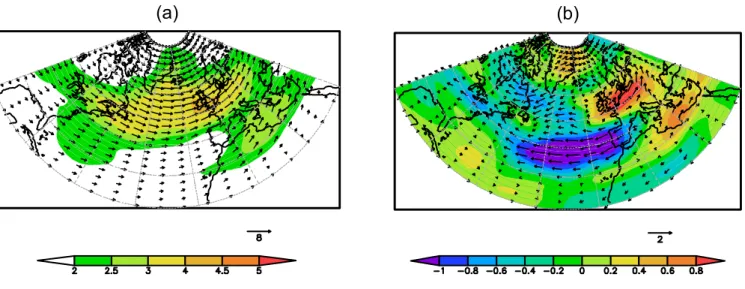
Fig. 3.Transient horizontal transports of momentumu′2ˆi+u′v′jˆat 300 hPa (vectors in 10−2m2s−2)for the:(a)dry winters;(b) differ-ence between the dry winters and the winter climatology. Shading represents the intensity of the fluxes in 10−2m2s−2.
31
(
j
ˆ
)
Fig. 4.The same as Fig. 3, but now for the transient horizontal transports of enthalpyu′T′ˆi+v′T′jˆat 300 hPa (in K m s−1).
enhanced positive forcing in the region upstream of the ridge and along the main storm track axis (Figs. 1 and 2). This pat-tern is very similar to the patpat-tern associated with the latent heat release (not shown). In fact, the large correspondence between the maxima of the diabatic heating and the maxima of the storm track are physically coherent with high precip-itation rates and nebulosity that are commonly found along the storm track, where significant amounts of latent heat are released in water vapour phase transitions (Black, 1998).
The transient horizontal enthalpy (Fig. 3) and momentum fluxes (Fig. 4), which are the basis for computing the third and sixth EFF components, reveal contrasting characteristics in the large-scale atmospheric flow. In effect, there is a
sig-nificant decrease in the intensity of the transports over the eastern North Atlantic for the dry winters when compared to climatology (negative anomalies in Figs. 3b, 4b), since regions of the maximum transports are concentrated in the preferred locations of the storm track (Lau and Nath, 1991). Again they are also plainly consistent with the presence of a strong North Atlantic ridge, blocking the westerly propaga-tion of the weather systems towards the Iberian Peninsula during dry winters. These results are in clear accordance with the results attained by Holopainen et al. (1982). Since the diabatic heating terms and the transient horizontal fluxes are directly related to the first, second, third and sixth EFF components (Eqs. 20, 21, 22 and 25), the above described
32
Fig. 5.Potential vorticity at 300 hPa (in 10−3s−1)and corresponding 300 hPa geopotential mean field (contours in 100 gpm) for the:(a)dry winters;(b)difference between the dry winters and winter climatology (in 10−5s−1).
33
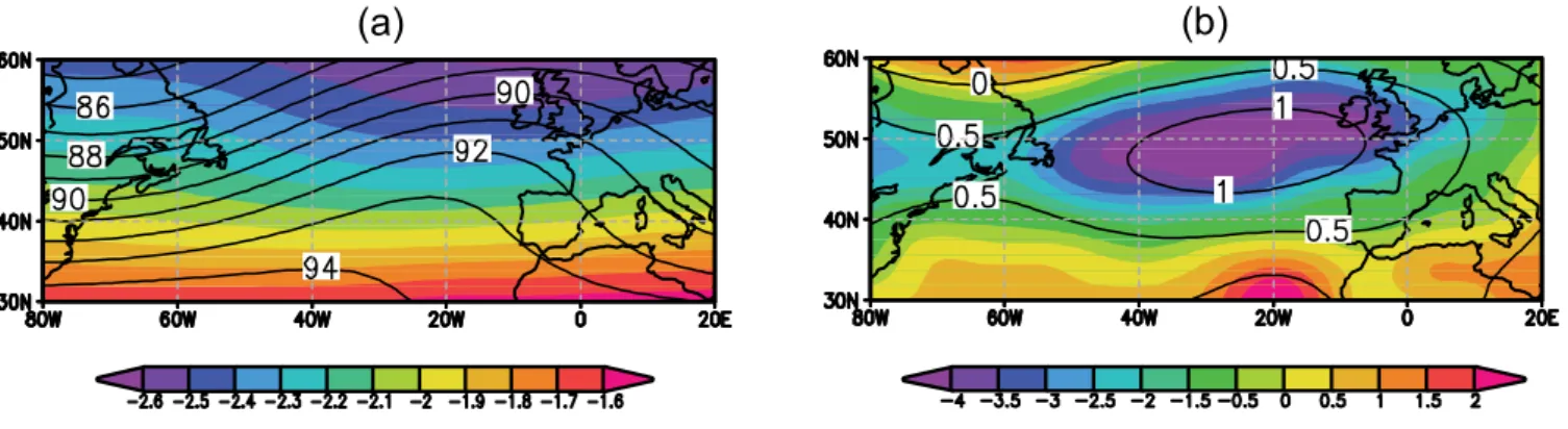
Fig. 6.Zonal cross-sections of the difference in the meridionally averaged (30◦N–60◦N) EFF pattern between the dry winters and winter climatology over the North Atlantic (80◦W–20◦E) and for the vertical layers(a)500–300 hPa (in 10−10s−2) and(b)1000–500 hPa (in 10−9s−2).
patterns significantly influence the EFF patterns. The verti-cal transient transports are not presented here as they showed to be of secondary relevance in the EFF computation (see next section).
4.3 Empirical Forcing Function
The composite potential vorticity field (Eq. 10) at 300 hPa for the dry winters and the corresponding deviations from the winter climatology are depicted in Fig. 5. By definition, this field tends to be proportional to minus the geopotential heights, explaining the negative values and the presence of a minimum in the area of the anticyclonic ridge and of a maxi-mum over the geopotential trough over the Western North
At-lantic (both fields tend to be in phase opposition). The strong meridional gradient of this field is still noteworthy (Fig. 5a). The anomalies depict a strong negative core over the North Atlantic within the range 45◦–55◦N (Fig. 5b), which is a clear manifestation of the anomalously enhanced ridge ob-served during the selected dry winters.
The zonal cross-sections of the EFF over the selected Euro-Atlantic sector (80◦W–20◦E) depict significant forc-ing values both at low (1000–500 hPa) and high tropo-spheric levels (500–300 hPa), though the near-surface forc-ing tends to have values one order of magnitude higher than at 300 hPa (Fig. 6). The high values of the low tropo-spheric forcing are coherent with the presence of very strong
34
Fig. 7.Vertically-averaged (500–300 hPa):(a)EFF pattern (in 10−10s−2);(b)third EFF component (in 10−11s−2);(c)sixth EFF compo-nent (in 10−11s−2)for the dry winters over the North Atlantic.
divergences/convergences at these levels due to diabatic pro-cesses that act as important factors in maintaining stationary-eddy potential vorticity. However, the cross-sections of the individual EFF components (not shown) reveal that the first component, which is associated with all diabatic heating pro-cesses but latent heat release, is the leading component not only at low tropospheric levels, but also at the upper tropo-sphere, with values at least one order of magnitude larger than the other EFF components. Hence, the EFF pattern mainly reflects the rate of total heat addition and therefore, as a first approximation, it can be estimated using only the first EFF component defined by Eq. (20).
The vertically-averaged (500–300 hPa) EFF pattern for the dry winters depicts an east-west dipolar structure over the North Atlantic (Fig. 7a), with essentially positive val-ues westwards of 40◦W of and an essentially negative val-ues eastwards. This pattern is thus plainly coherent with the presence of a strong North Atlantic ridge during the selected winters, since the stationary-eddy cyclonic potential vorticity (positive EFF values) tends to be associated with geopoten-tial troughs, while the stationary-eddy anticyclonic potengeopoten-tial vorticity (negative EFF values) tends to be associated with geopotential ridges. Despite the leading role of the first com-ponent in maintaining the stationary-eddy potential vorticity,
the second component, associated to latent heat release, is also important at low tropospheric levels, where humidity is essentially concentrated (not shown). Conversely, at higher tropospheric levels, the third and sixth components acquire a (relatively) higher relevance, documenting the relevance of the transient enthalpy and momentum transports in the main-tenance of the stationary-eddy flow. These results are coher-ent with previous results using the Eliassen-Palm fluxes (cf., Fig. 9, Santos et al., 2009b).
The third and sixth components of the vertically averaged EFF at high tropospheric levels (500–300 hPa) for the dry winters (Fig. 7b–c) reveal physically meaningful patterns. In the third EFF component for dry winters (Fig. 7b), the strong negative core over the North Atlantic is noteworthy. This pattern clearly supports the maintenance of the anoma-lously strong ridges. In the sixth EFF component, there is a very pronounced sequence of strong forcing cores along the northern border of the ridge (Fig. 7c). In fact, these forcing cores play an important role in aligning the eddy-driven polar jet and the storm track along their maxima by maintaining a sequence of positive and negative potential vorticity anoma-lies (Holopainen et al., 1982). Overall, the transient trans-ports of both enthalpy and momentum at higher tropospheric levels are then shown to be essential for the maintenance of
the large-scale asymmetric anomalies over the North Atlantic (Lau and Nath, 1991). The fourth and seventh components, associated with the vertical transient fluxes, are negligible throughout the troposphere (not shown) and can be generally discarded from the calculations of the EFF.
5 Discussion and conclusions
The formulation of the time-mean potential vorticity equa-tion on isobaric surfaces (after Saltzman, 1962) is revis-ited in the present study. This less conventional formulation presents some attractive features. This formal development comprises a forcing term of the equation (EFF) that can be decomposed into seven additive components associated with different physical mechanisms. The role of different inter-nal forcing mechanisms (both thermal and mechanical pro-cesses) in maintaining stationary eddies in the large-scale at-mospheric motion can then be assessed.
The EFF was applied as a tool to diagnose large-scale sta-tionary eddies associated with the occurrence of strong ridges over the Eastern North Atlantic, which are often precursors of severe droughts over Western Iberia. Results show that the EFF pattern (total forcing term) is dynamically coherent with the configuration of the geopotential height field. For such events, the EFF pattern depicts a clear dipolar struc-ture over the North Atlantic that contributes to the mainte-nance of cyclonic (anticyclonic) potential vorticity upstream (downstream) of the anomalously strong ridges. The analy-sis of the individual components also shows that among the six calculated components (the fifth EFF component is asso-ciated to frictional effects and was not computed), the most important component throughout the troposphere is the first one, which is associated with diabatic heating (latent heat excluded). Nevertheless, latent heat release (second com-ponent) can also be important at low tropospheric levels, while transient horizontal enthalpy (third component) and momentum (sixth component) fluxes are important at high tropospheric levels. When compared with the latter com-ponents, vertical fluxes are negligible throughout the tropo-sphere (fourth and seventh components). As such, the EFF pattern can be, at a first approximation, accurately estimated by computing only the first component. At a second approx-imation, the estimation of the EFF pattern at low (high) tro-posphere can be further improved by considering the second (third and sixth) components. No significant improvements can be made when considering the remaining components. Hence, they may be discarded in future studies.
Despite the previous results, in the interpretation of the EFF patterns some considerations must be born in mind. Al-though several internal (both mechanical and thermal) pro-cesses are taken into account in the EFF definition, the ex-ternal forcing mechanisms of the atmospheric circulation, such as topographic effects, diabatic fluxes at the lower at-mospheric boundary are not incorporated in this definition.
In fact, these processes can only be included as boundary conditions. Furthermore, taking into account that the EFF formulation derives from the equation of the time-mean po-tential vorticity over a relatively long time scale (e.g., a sea-son), the EFF analysis only allows a diagnostic approach to the dynamical conditions, not enabling studies of gener-ation/decay (development) of the anomalies. In fact, in this kind of analysis it can only be stated that an EFF compo-nent can contribute or not for the maintenance of a specific stationary eddy. Many previous studies have shown that tran-sient eddies interact through positive and negative feedback mechanisms with the mean flow and cannot be considered as independent forcing entities of the atmospheric flow (e.g., Rivi`ere, 2009).
Even taking into consideration the previous limitations of the EFF analysis, results give some evidence for considering the EFF patterns as a valuable tool in diagnosing stationary-eddy anomalies in the large-scale atmospheric motion, il-lustrated here for the occurrence of strong ridges over the Eastern North Atlantic. Moreover, by definition, the EFF enables the assessment of the different contributions made by internal (both mechanical and thermal) atmospheric pro-cesses in the maintenance of time-mean (e.g., seasonal mean) axially asymmetric anomalies in the atmospheric flow. This last property is a major motivation to consider the EFF pat-terns when analysing other large-scale atmospheric anoma-lies (e.g. teleconnections), which can be dealt with in future studies.
Appendix A
Mathematical development of EFF
The aim of this section is to guide the reader interested in the details involving the intricate mathematical development of the EFF. This development comprises the intermediate steps of the deduction between relation (11) and (15) of Sect. 2.1.
The following relations are going to be included during the mathematical development of the EFF. Let us considered the absolute vorticity equation,η,
η=ζ+f, (A1)
from which the next equalities are obtained
ω∂η ∂p =ω
∂ (ζ+f ) ∂p
=ω∂ζ
∂p (A2)
and
η∇ •v=(ζ+f )∇ •v
= −ζ∂ω ∂p−f
∂ω
∂p (A3)
From the potential vorticity definition (10) the following con-ditions are attained
∂ ∂t f ∂ ∂p T Ŵ
=f ∂ ∂t 1 Ŵ ∂T ∂p −f ∂ ∂t T Ŵ2 ∂Ŵ ∂p , (A4)
v• ∇5=v• ∇η+v• ∇
f ∂ ∂p T Ŵ , (A5) v•∇ f ∂ ∂p T Ŵ
=fv•∇ ∂ ∂p T Ŵ + ∂ ∂p T Ŵ
v•∇f,(A6) and v•∇ f ∂ ∂p T Ŵ
=fv•∇
1 Ŵ ∂T ∂p
−fv•∇
T Ŵ2 ∂Ŵ ∂p .(A7) Let us also considered the following equalities
∂ ∂p
T
Ŵ
v• ∇f= −T Ŵ2
∂Ŵ
∂pv• ∇f, (A8)
f ∂ ∂p
1
Ŵv• ∇T
= f Ŵ
∂v ∂p• ∇T+
f Ŵv•
∂ ∂p∇T
−fv• ∇
T Ŵ2
∂Ŵ
∂p, (A9)
−fv Ŵ2
∂
∂p(T• ∇Ŵ)= −f ∂ ∂p
T Ŵ2v• ∇Ŵ
+f T Ŵ2
∂v ∂p• ∇Ŵ,
(A10) and ∂ ∂p T Ŵv• ∇f
=fv• ∇
1 Ŵ ∂T ∂p −f Ŵv•
∂
∂p∇T . (A11)
From the energy conservation Eq. (5)
ω= Q Ŵcp
−1 Ŵ
∂T
∂t +v• ∇T
. (A12)
Let us remind that in Sect. 2.1. from vorticity Eq. (13) the following equality (14) was attained
∂η ∂t
|{z}
(11)
+v• ∇η
| {z }
(12)
+ω∂η
∂p+η∇ •v+k∇ω× ∂v
∂p−k• ∇ ×F
+∂ ∂t f ∂ ∂p T Ŵ
| {z }
(11)
+v• ∇
f ∂ ∂p T Ŵ
| {z }
(12) = ∂ ∂t f ∂ ∂p T Ŵ
+v• ∇
f ∂ ∂p T Ŵ therefore ∂5
∂t +v• ∇5= ∂ ∂t f ∂ ∂p T Ŵ
+v• ∇
f ∂ ∂p T Ŵ −ω∂η ∂p
| {z }
(A2)
−η∇ •v
| {z }
(A3)
−k∇ω×∂v
∂p+k• ∇ ×F
(A13)
after substituting the expressions
∂5
∂t +v• ∇5= ∂ ∂t f ∂ ∂p T Ŵ
| {z }
(A4)
+v• ∇
f ∂ ∂p T Ŵ
| {z }
(A6)
−ω∂ζ ∂p+ζ
∂ω ∂p+f
∂ω ∂p
| {z }
(A12)
−k∇ω×∂v
∂p+k• ∇ ×F
(A14) consequently
∂5
∂t +v• ∇5= −f ∂ ∂p T Ŵ2 ∂Ŵ ∂t +f ∂ ∂p 1 Ŵ ∂T ∂t
+f v• ∇ ∂ ∂p
T Ŵ
| {z }
(A7) + ∂ ∂p T Ŵ
v• ∇f
| {z }
(A8)
−ω∂ζ ∂p+ζ
∂ω ∂p+f
∂ ∂p Q Ŵ − f ∂ ∂p 1 Ŵ ∂T ∂t
−f ∂ ∂p
1
Ŵv• ∇T
| {z }
(A9)
−k∇ω×∂v
∂p+k• ∇ ×F (A15)
from which after some simplifications the next equality is attained
∂5
∂t +v• ∇5= −f ∂ ∂p T Ŵ2 ∂Ŵ ∂t
+fv• ∇
1 Ŵ ∂T ∂p
| {z }
(A11)
−f Ŵ2v•
∂T ∂p∇Ŵ
| {z }
(A10) −ω∂ζ ∂p+ζ ∂ω ∂p+f ∂ ∂p Q Ŵ −f Ŵ ∂v ∂p• ∇T−
f Ŵv•
∂ ∂p∇T
| {z }
(A11)
−k∇ω×∂v ∂p
+k• ∇ ×F (A16)
From Eq. (A16) substituting Eq. (A10) the following relation is attained
∂5
∂t +v• ∇5= −f ∂ ∂p T Ŵ2 ∂Ŵ ∂t + ∂ ∂p T Ŵ
v• ∇f
−f ∂ ∂p
T Ŵ2v• ∇Ŵ
+f T Ŵ2
∂v ∂p• ∇Ŵ
−ω∂ζ ∂p+ζ ∂ω ∂p+ f ∂ ∂p Q Ŵ −f Ŵ ∂v
∂p• ∇T−k∇ω× ∂v ∂p
+k• ∇ ×F (A17)
after taking the time-mean relations (15) and (16) are ob-tained and therefore equality (17)
∂5
∂t +v• ∇5=f ∂ ∂p
Q Ŵ
!
+k• ∇ ×F+non-linear terms
=2+non-linear terms
Appendix B
Notation used in the text
λ Longitude
ϕ Latitude
p Pressure
t Time
a=6.371×10⁶m Mean radius of the earth
=7.292×10⁻⁵rad s−1 Angular velocity of the Earth
g=9.80 ms−2 Apparent gravity accelera-tion
u=acosϕdλdt Zonal wind component
v=adϕdt Meridional wind
compo-nent
v=ui+vj Horizontal wind
ω=dpdt Omega-vertical wind
com-ponent
8=gz Geopotential
T Air temperature
cp=1004 J kg−1K−1 Specific heat at constant pressure
R=287 J kg−1K−1 Gas constant for dry air
Fλ Specific eastward/zonal
frictional force
Fϕ Specific
north-ward/meridional frictional force
q Specific humidity
˙
qF Specific diabatic heating
rate due to conduction and friction
˙
qR Specific diabatic heating
rate due to radiation
˙
qL Specific diabatic heating
rate due to latent heat re-lease
Ŵ Static stability parameter
2 Empirical forcing function
ffn n-th component of the
em-pirical forcing function
() Time-mean
()′=()−() Departure from time-mean
hi Zonal-mean
()∗=()− hi Departure from zonal-mean
Acknowledgements. This work was supported by the project “Connections between precipitation extremes in Southern Europe and large-scale climate variability” (CRUP N A-28/08; DAAD D/07/13642). All maps were produced by the Grid Analysis and Display System developed at the Center for Ocean-Land-Atmosphere Interactions. The authors are grateful to the two excel-lent reviewers who significantly contributed to improve the paper.
Topical Editor F. D’Andrea thanks two anonymous referees for their help in evaluating this paper.
References
Basset, H. A. and Ali, A. M.: Diagnostic of Cyclogenesis using Potential Vorticity, Atmosfera, 19(4), 213–234, 2006.
Black, R.: The Maintenance of Extratropical Intraseasonal Tran-sient Eddy Activity in the GEOS-1 Assimilated Dataset, J. At-mos. Sci., 55, 3159–3175, 1998.
Blackmon, M. L.: A climatological spectral study of the 500 mb geopotential height of the Northern Hemisphere, J. Atmos. Sci., 33, 1607–1623, 1976.
Blackmon, M. L., Lee, Y. H., and Wallace, J. M.: Horizontal struc-ture of 500 mb height fluctuations with long, intermediate and short time scales, J. Atmos. Sci., 41, 961–979, 1984a.
Blackmon, M. L., Lee, Y.-H., Wallace, J. M., Hsu, H.-H.: Time Variation of 500 mb Height Fluctuations with Short, Medium and Long Time Scales, J. Atmos. Sci., 41, 981–991, 1984b. Blackmon, M. L., Wallace, J. M., Lau, N.-C., and Mullen, S. L.:
An observational study of the Northern hemisphere wintertime circulation, J. Atmos. Sci., 34, 1040–1053, 1977.
Bluestein, H. B.: Synoptic-Dynamic Meteorology in Middle Lati-tudes, Oxford University Press, Vol. II, 1993.
Chang, E. K. M. and Fu, Y.: Interdecadal variations in Northern Hemisphere winter storm track intensity, J. Climate, 22, 670– 688, 2002.
Chang, E. K. M.: Diabatic and Orographic Forcing of Northern Winter Stationary Waves and Storm Tracks, J. Climate, 15, 642– 658, 2009.
Charney, J. G.: The dynamics of long waves in a barocline westerly current, J. Meteorol., 4, 135–163, 1947.
Chen, P., Hoerling, M., and Dole, R.: The Origin of the Subtropical Anticyclones, J. Atmos. Sci., 58, 1827–1835, 2001.
Christoph, M., Ulbrich, U., and Haak, U.: Faster Determination of the Intraseasonal Variability of Storm tracks Using Murakami’s Recursive Filter, Mon. Weather Rev., 123, 578–581, 1995. Davis, R. E., Hayden, B. P., Gay, D. A., Phillips, W. L., and Jones,
G. V.: The North Atlantic Subtropical Anticyclone, J. Climate, 10, 728–744, 1997.
Eady, E. T.: Long waves and cyclone waves, Tellus, 1, 33–52, 1949. Edmon, H. J., Hoskins, B. J., and McIntyre, M. E.: Eliassen-Palm cross sections for the troposphere, J. Atmos. Sci., 37, 2600–2616, 1980.
Ertel, E.: Ein neuer hydrodynamischer Wirbelsatz, Meteor. Z., 59, 277–281, 1942.
Garc´ıa-Herrera, R., Paredes, D., Trigo, R., Trigo, I., Hern´andez, E., Barriopedro, D., and Mendes, M.: The Outstanding 2004/05 Drought in the Iberian Peninsula: Associated Atmospheric Cir-culation, J. Hydrometeorol., 8, 483–498, 2007.
Hanson, C. E., Palutikof, J. P., Livermore, M. T. J., Barring, L., Bindi, M., Corte-Real, J., Duaro, R., Giannakopoulos, C., Good,
P., Holt, T., Kundzewicz, Z., Leckebush, G., Moriondo, M., Radziejewski, M., Santos, J., Schlyter, P., Schwarb, M., Stjern-quist, I., and Ulbrich, U.: Modelling the Impact of Climate Ex-tremes: An overview of the Project, Prudence Special Issue, Clim. Change, 81, (1), 163–177, 2007.
Hartmann, D. H.: On potential vorticity and transport in the strato-sphere, J. Atmos. Sci., 34, 968–977, 1977.
Holton, J. R.: An Introduction to Dynamic Meteorology, Elsevier, 2004.
Holopainen, E., Ronto, L., and Lau, N.: The Effect of Large-Scale Transient Eddies on the Time-mean flow in the Atmosphere, J. Atmos. Sci., 39, 1972–1984, 1982.
Hoskins, B. J., McIntyre, M. E., and Robertson, A. W.: On the Use of Significance of Isentropic Potential Vorticity Maps, Q. J. Roy. Meteorol. Soc., 111(470), 877–946, 1985.
Hoskins, B. J. and Valdes, P. J.: On the existence of storm tracks, J. Atmos. Sci., 47, 1854–1864, 1990.
Hurrell, J. W.: Decadal Trends in the North Atlantic Oscillation: Regional Temperatures and Precipitation, Science, 269, 676– 679, 1995.
Kistler, R., Kalnay, E., Collins, W., et al.: The NCEP/NCAR 50-Year Reanalysis: Monthly-Means CD-ROM and Documentation, B. Am. Meteorol. Soc., 82, 247–267, 2001.
Lau, N. and Nath, M.: Variability of the Baroclinic Transient Eddy Forcing Associated with Monthly Changes in the Midlatitude Storm Tracks, J. Atmos. Sci., 48, 2589–2613, 1991.
Lau, N. and Wallace, J. M.: On the distribution of horizontal trans-ports by transient eddies in the northern wintertime circulation., J. Atmos. Sci., 36, 1844–1861, 1979.
Lolis, C. J., Metaxas, D. A. and Bartzokas, A.: On the Intra-annual Variability of Atmospheric Circulation in Mediterranean Region, Int. J. Climatol., 28, 1339–1355, 2008.
Mendes, D. and Mendes, M. D.: Climatology of cyclones, anticy-clones and storm tracks: revision of concepts, Rev. Bras. Geof., 22(2), 127–134, 2004.
Peixoto, J. P. and Oort, A. H.: Physics of Climate, American Insti-tute of Physics, New York, 1992.
Pinto, J. G., Ulbrich, U., Leckebush, G. C., Spangehl, T., Reyes, M., and Zacharias, S.: Changes in storm track and cyclone activity in three SRES ensemble experiments with the ECHAM5/MPI-OM1 GCN, Clim. Dynam., 29, 195–210, 2007.
Rivi`ere, G.: Effect of Latitudinal Variations in Low-Level Baro-clinicity on Eddy Life Cycles and Upper-Tropospheric Wave-Breaking Processes, J. Atmos. Sci., 66, 1569–1592, 2009. Salby, M. and Roger, P.: Fundamentals of Atmospheric Physics,
Elsevier, Academic Press, 1996.
Saltzman, B.: Empirical Forcing Functions for the Large-Scale Mean Disturbances in the Atmosphere, Pure Appl. Geophys., 52, 173–188, 1962.
Santos, J. and Corte-Real, J.: Temperature Extremes in Europe and Large-Scale Circulation: HadCM3 future scenarios, Clim. Res., 31(1), 3–18, 2006.
Santos, J., Corte-Real, J., and Leite, S.: Weather regimes and their connection to the winter rainfall in Portugal, Int. J. Climatol., 25(1), 33–50, 2005.
Santos, J. and Leite, S.: Long-term variability of the temperature time series recorded at Lisbon, J. App. Stat., 36(3), 323–337, doi:10.1080/02664760802449159, 2009a.
Santos, J., Andrade, C., Corte-Real, J., and Leite, S.: The role
of large-scale eddies in the occurrence of winter precipitation deficits in Portugal, Int. J. Climatol., 29(10), 1493–1507, 2009b. Santos, J., Corte-Real, J., and Leite, S.: Atmospheric Large-scale Dynamics During the 2004–2005 Winter Drought in Portugal, Int. J. Climatol., 27(5), 571–586, 2007a.
Santos, J., Corte-Real, J., Ulbrich, U., and Palutikof, J.: European Winter Precipitation Extremes and Surface Large-Scale Circula-tion: a Coupled Model and its Scenarios, Theor. Appl. Climatol., 87(1–4), 85–102, 2007b.
Santos, J. A., Pinto, J. G., and Ulbrich, U.: On the development of strong ridge episodes over the eastern North Atlantic, Geophys. Res. Lett., 36, L17804, doi:10.1029/2009GL039086, 2009c. Savij¨arvi, H.: The interaction of the Monthly mean flow and
large-scale transient eddies in two different types. Part III: Potential vorticity balance, Geophysica, 15, 1–16, 1978.
Stephenson, D. B. and Held, I. M.: GCM response of northern win-ter stationary waves and storm tracks to increasing amounts of carbone dioxide, J. Climate, 6, 1859–1870, 1993.
Tank, A. M. G. K., Wijngaard, J. B., Konnen, G. P., Bohm, R., Demaree, G., Gocheva, A., Mileta, M., Pashiardis, S., Hejkr-lik, L., Kern-Hansen, C., Heino, R., Bessemoulin, P., Muller-Westermeier, G., Tzanakou, M., Szalai, S., Palsdottir, T., Fitzger-ald, D., Rubin, S., Capaldo, M., Maugeri, M., Leitass, A., Bukan-tis, A., Aberfeld, R., Van Engelen, A. F. V., Forland, E., Mietus, M., Coelho, F., Mares, C., Razuvaev, V., Nieplova, E., Cegnar, T., Lopez, J. A., Dahlstrom, B., Moberg, A., Kirchhofer, W., Cey-lan, A., Pachaliuk, O., Alexander, L. V., and Petrovic, P.: Daily dataset of 20th-century surface air temperature and precipitation series for the European Climate Assessment, Int. J. Climatol., 22, 1441–1453, 2002.
Trewartha, G. T. and Horn, L. H.: An Introduction to Climate, McGraw-Hill, 1980.
Ulbrich, U., Christoph, M., Pinto, J. G., and Corte-Real, J.: Depen-dence of Winter Precipitation over Portugal on NAO and Baro-clinic Wave Activity, Int. J. Climatol., 19, 379–390, 1999. Ulbrich, U., Pinto, J. G., Kupfer, H., Leckebusch, G. C., Spangehl,
T., and Reyers, M.: Changing Northern Hemisphere Storm Tracks in an Ensemble of IPCC Climate Change Simulations, J. Climate, 21, 1669–1679, 2008.
Wang, C.: Atlantic Climate Variability and Its Associated Atmo-spheric Circulation Cells, J. Climate, 15, 1516–1536, 2002. Wallace, J. M. and Gutzler, D. S.: Teleconnections in the
geopoten-tial height field during the Northern Hemisphere Winter, Mon. Weather Rev., 109, 784–812, 1981.
Wallace, J. M., Lim, G., and Blackmon, M. L.: Relationship be-tween Cyclone Tracks, Anticyclone Tracks and Barocline Wave Guides J. Atmos. Sci., 45, 439–462, 1988.
Wallace, J. M. and Hobbs, P. V. : Atmospheric Science: An Intro-ductory Survey, Elsevier, 2006.
Wiin-Nielsen, A.: On the Structure of Atmospheric Waves in Mid-dle Latitudes, Atmosfera, 16, 83–102, 2003.
WMO: Climatological Normals (CLINO) for the Period 1961– 1990, World Meteorological Organization Doc. WMO/OMM, 847, Geneva, 1996.
Yin, J. H.: A Consistent Poleward Shift of the Storm Tracks in Sim-ulations of 21st Century Climate, Geophys. Res. Lett., 32, 18, doi:10.1029/2005GL023684, 2005.