urban rail transit
Xinmiao Zhao, Quanxin Sun, Yuting Zhu, Yong Ding,
Cunrui Ma and Zhijie Chen
Abstract
A Y-type urban rail transit is composed of a trunk and a branch, and the passenger demand has the characteristics of mul-tidirectional and unbalanced. It is important to design routing planning of Y-type urban rail transit and provide reasonable service for passengers with acceptable operational cost. In this study, a routing planning design model was proposed for Y-type urban rail transit aimed at minimizing the passenger travel time and train operating distance. The decision vari-ables of the model were the locations of turn-backs and the departure frequencies of the train routings in the multi-routing planning. The constraints of passenger demand and line condition were considered. The multi-objective model was turned into a single-objective model by giving weight values to the objectives. Then a genetic algorithm was applied to obtain optimal solutions of the proposed model. Finally, a case study was conducted, and the optimal solutions under different forms of multi-routing planning with different weight values were analyzed. The results showed that when the weight of the passenger travel time increased to a certain level, the optimal solution changed from a two-routing plan-ning to a three-routing planplan-ning, and the latter one could better meet the characteristics of the passenger.
Keywords
Urban rail transit, Y-type line, routing planning, multi-routing, passenger demand
Date received: 15 April 2016; accepted: 8 August 2016
Academic Editor: Anto´nio Mendes Lopes
Introduction
Y-type lines are those lines starting as heavily traveled trunk lines from the city center outward and then divid-ing into a greater number of lines with lower loads ser-ving large, often low-density areas.1 Y-type lines can attract more passengers to increase profit by expanding service areas, so the adoption of multi-routing mode may make the train routing planning better satisfy the multidirectional and unbalanced characteristics of pas-senger demand. There are many Y-type urban rail tran-sit lines in operation such as Paris Line RER-A, Munich Metro Line 3 and Line 6, Guangzhou Metro Line 3, Beijing Subway Line Yanfang, and Hangzhou Metro Line 1.
Designing train planning of Y-type urban rail transit is to determine the locations of turn-backs and
frequencies of the train routings subject to passenger demand and line condition. There exists much research on multi-routing planning in the field of urban public transport and railway; Furth2and Furth and Day3 pro-pose methods on designing routing planning subject to a certain scale of vehicles and a balanced load factor, and propose the conception ‘‘schedule mode’’ which is the rate of the routings’ departure frequencies to cope
MOE Key Laboratory for Urban Transportation Complex Systems Theory and Technology, Beijing Jiaotong University, Beijing, China
Corresponding author:
Xinmiao Zhao, MOE Key Laboratory for Urban Transportation Complex Systems Theory and Technology, Beijing Jiaotong University, No. 3 Shangyuancun, Haidian District, Beijing 100044, China.
Email: [email protected]
with cyclical diagram; Ceder and colleagues4–6propose a multi-routing planning model aimed at minimizing the number of vehicles and the number of short-turn trips, and a strategy which combines short-turning, holding, and stop-skipping to reduce the passenger travel time and passenger transfers; Vijayaraghavan and Anantharamaiah7propose to insert deadhead trips to meet passenger demand and reduce the number of
vehicles; Tirachini and colleagues8,9 and Site and
Filippi10 propose a strategy combining short-turn and expressing to analyze the effects of departure frequen-cies, vehicle sizes, and turn-back stations on passengers and operator when the arrival of buses follows uniform distribution, and also Site and Filippi10study the situa-tion when the arrival of buses follows Poisson’s distri-bution; Canca et al.11 propose a short-turn strategy to solve disruptions caused by heavy demand, aimed at diminishing passenger waiting time while preserving the quality of service; Jannson12 optimizes the departure frequency and vehicle size to reduce passenger travel cost and operator cost; Chen et al.13 design an algo-rithm which can adjust train operation based on ordi-nary optimization and took a heavy haul railway as an example to prove that the solution can well satisfy the passenger demand.
However, the studies mentioned mainly focus on sin-gle lines, whose passengers do not need to transfer because all demands can be covered by the full-length routing which covers all the stations. However, the pas-senger demand of a Y-type line cannot be satisfied by a full-length routing, especially when the line connects the city center with the suburbs, so there exist some passengers who need to transfer. Also, the departure frequencies of the routings on the trunk line and the branch line are subject to the tracking interval because of the routings’ joint operation, which means different kinds of services operate on the same line. Therefore, the existing studies on single lines are not suitable for a Y-type line. The routing planning of Y-type line has been studied by a limited number of authors, and the studies mainly focus on designing the trunk line and branch line,14 proposing the variants of routing plan-ning by qualitative description15 and optimizing the vehicle circulation under a certain routing planning.16
In summary, the studies on multi-routing planning did not consider the characteristics of Y-type line, and the studies on Y-type lines did not consider the influ-ence of the departure frequencies and the turn-back stations. Thus, this article proposed a multi-routing planning model aimed at minimizing the passenger travel time and operator cost. Then the optimal solu-tions under different weights of passenger travel cost were obtained, and the influence of different types of routing planning on the passengers and the operator was discussed.
Description of the problem
Y-type line is usually composed of a trunk line and a branch line connected by a node station shown in Figure 1, in which O is the node station, AOB is the trunk line (named Trunk), and OC is the branch line (named Branch). Usually, the passenger flow of the trunk is larger than that of the branch.
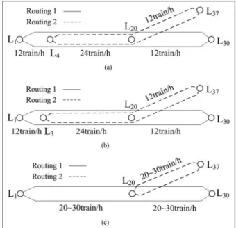
The typical forms of multi-routing planning of Y-type line include separate operation, straight-through operation, and integrated operation which is a combi-nation of the previous two forms. There are three com-binations under two-routing planning, as shown in Figure 2(a)–(c). However, the combinations under three-routing planning are related to the relationships of the turn-backs of different routings. Thus, the com-binations are numerous and several comcom-binations are shown in Figure 2(d)–(f) because of the limitation of space.
A routing planning with two routings is called two-routing planning, such as Figure 2(a)–(c); a two-routing planning with three routings is called three-routing planning, such as Figure 2(d)–(f). Most of the cases in use adopt a two-routing planning because the operation is not as complex as three-routing planning, but the diversity of three-routing planning may make it better meet the complex and unbalanced passenger demand, which may bring some additional profit to the passen-gers or the operator. Therefore, this article studied multi-routing planning of Y-type urban rail transit. The variables are the departure frequencies and the turn-back stations of the routings under the constraints of passenger demand and line condition, aiming at minimizing the passenger travel time and operator cost.
The article is organized as follows: sections
‘‘Description of the problem’’ and ‘‘Modeling’’ describe the problem and the modeling, respectively; section ‘‘Solution algorithm’’ describes the algorithm; section
‘‘Case study’’ studies on a case and section
‘‘Conclusion’’ concludes the article.
Modeling
The typical multi-routing planning of two-routing and
three-routing are shown in Figures 3 and 4,
respectively.
The routing covering all the stations on the trunk AOB is the trunk routing, called Routing 1; the routing covering the branch OC is the branch routing, called
Routing 2. Routing 2 may covers some stations on AO, too; if there are three routings, the third one is a minor routing, called Routing 3. Therefore, Routing h is used to represent the routings, andh(h= 1, 2, 3) is the order number of the routing. The turn-back stations of
Routing 1 are L1 and Lm; the turn-back stations
of Routing 2 areLx andLn; the turn-back stations of Routing 3 areLyandLz, and the departure frequency of Routinghisfh(h= 1, 2, 3).
When f36¼0, the planning is three-routing; when
f3= 0, the planning is two-routing, and the planning is
separate operation when Lx= Lb while
straight-through operation whenLx= L1, so the routing
plan-ning in Figure 4 can contain the variants shown in Figure 2. The major variables, parameters, and nota-tions used in this article are shown in Tables 1–3, respectively.
The multi-routing planning of Y-type line is com-plex, so the following assumptions were used to sim-plify the problem:
1. The passenger flow of the trunk is usually larger than the branch, which is easier to show the characteristic of unbalanced. Thus, the minor routing (Routing 3) was assumed on the trunk line if it existed.
2. Passengers would not choose routings with
transfers unless they had to. 3. The trains’ formation was fixed.
4. The arrival of passengers was assumed to follow uniform distribution under large passenger flow with short intervals.
5. Passengers boarded and alighted at the stations simultaneously, and the boarding process was slower. Thus, the stop time of a train at each sta-tion was assumed to be equal to the boarding time with an upper limit and a lower limit. 6. Considering the saturated capacity of a subway at
the peak hour, the departure frequencies of differ-ent routings were assumed to have multiple rela-tionships with each other, which could ensure balanced headways under a certain level of service.
The designing of routing planning affects the service quality for the passengers and the operational cost of the operator. Therefore, this article proposed a model considering both the travel time of the passengers and the operating distance of the trains to represent service quality and operational cost. Also, the constraints such
Figure 2. Typical multi-routing planning of Y-type line: (a) separate operation, (b) straight-through operation, (c) integrated operation under two-routing, (d) integrated operation 1 under three-routing, (e) integrated operation 2 under three-routing, and (f) integrated operation 3 under three-routing.
Figure 3. Routing planning of two-routing.
as turn-back tracks of stations, transport capacity and passenger demand, and tracking interval were consid-ered. Finally, the optimal solutions of routing planning were obtained.
Passenger travel time
The passenger travel time was composed of waiting time, in-vehicle time, and transfer time. Waiting time was the product of passenger flow and average waiting time; in-vehicle time was the product of passenger flow
and section running time, station stop time; transfer time was the product of transfer passenger flow and average transfer time. The passenger travel time is expressed as follows
Z1=CW+CV+CT ð1Þ
In whichZ1is the passenger travel time (s),CWis the
passenger waiting time (s), CV is the passenger
in-vehicle time (s), and CT is the passenger transfer time (s).
Table 1. Variables and definitions.
Variables Definition
Lx Unknown turn-back station of Routing 2; decision variable
Ly Unknown turn-back station of Routing 3 with a smaller order number; decision variable
Lz Unknown turn-back station of Routing 3 with a larger order number; decision variable
fh Departure frequencies of Routingh(h= 1, 2, 3) in the research periodT, train/h; decision variable
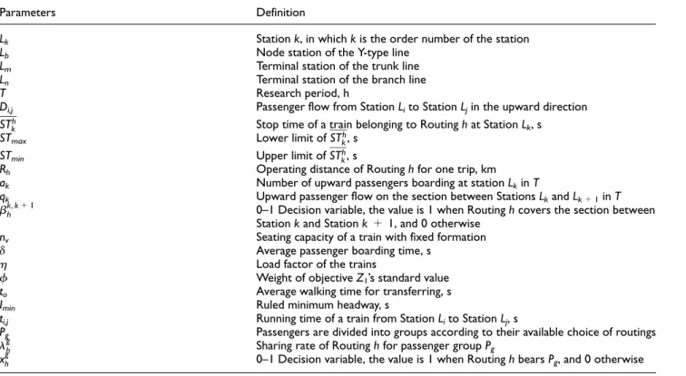
Table 2. Parameters and definitions.
Parameters Definition
Lk Stationk, in whichkis the order number of the station
Lb Node station of the Y-type line
Lm Terminal station of the trunk line
Ln Terminal station of the branch line
T Research period, h
Di,j Passenger flow from StationLito StationLjin the upward direction
STh
k Stop time of a train belonging to Routinghat StationLk, s
STmax Lower limit ofSTkh, s
STmin Upper limit ofSThk, s
Rh Operating distance of Routinghfor one trip, km
ak Number of upward passengers boarding at stationLkinT
qk Upward passenger flow on the section between StationsLkandLk+1inT bkh,k+1 0–1 Decision variable, the value is 1 when Routinghcovers the section between
Stationkand Stationk+1, and 0 otherwise
nv Seating capacity of a train with fixed formation
d Average passenger boarding time, s
h Load factor of the trains
f Weight of objectiveZ1’s standard value
to Average walking time for transferring, s
Imin Ruled minimum headway, s
ti,j Running time of a train from StationLito StationLj, s
Pg Passengers are divided into groups according to their available choice of routings
lgh Sharing rate of Routinghfor passenger groupPg
xgh 0–1 Decision variable, the value is 1 when RoutinghbearsPg, and 0 otherwise
Table 3. Notations and definitions.
Notations Definition
H Order number of routings. Routing 1, Routing 2, and Routing 3 are, respectively, expressed ash=1,h=2, andh=3
Z1 Objective 1, passenger travel time inT, s
Z2 Objective 2, train operating distance inT, km
CW Passenger waiting time inT, s
CV Passenger in-vehicle time inT, s
CT Passenger transfer time inT, s
Waiting time. The location of a station determines the service frequencies for the passengers at the station, for example, in Figure 3, Stations L1–Lx and Lb–Lm are
only covered by Routing 1, Stations Lb–Ln are only
covered by Routing 2, and StationsLx–Lbare covered by both routings. For ease of expression, the Y-type line is divided into at most six passenger segments shown in Figure 5 according to the location of turn-back stations, and this way of division can cover other situations, such as whenLx=Lb, it would be separate operation, and Segment 2 no longer exists; when Lx=L1, it would be straight-through operation, and
Segment 1 no longer exists. The passenger flow from
Segment 1 to Segment 2 is expressed as
c12=Px 1 i=1
Pb
j=xDi,j, and so on.
A passenger’s choice for the routings is dependent on his or her OD (origin station and destination sta-tion), such as passengers from Segment 1 to Segment 6 in Figure 5 need to transfer from Routing 1 to Routing 2, while passengers from Segment 2 to Segment 6 only need to catch Routing 2. According to Assumption 2, passengers were divided into groups namedPg: P1needed to catch Routing 1;P2needed to
catch Routing 2;P3could catch Routing 1 or Routing
2;P4could catch Routing 1 or Routing3;P5could catch
Routing 1, Routing 2, or Routing 3. In this section, the waiting time of the passengers who need to transfer only accounts for the waiting time for the first routing they catch, and the waiting time for the routing after transfer-ring would be calculated in section ‘‘Tranfer time’’. Thus, the expressions ofPgare as follows
P1=
Xx
1
i=1
Xn
i+1
Di,j+
X
y1
i=x
Xm
j=z
Di,j+
Xz
i=y
Xm
j=z+1
Di,j
+ X
m1
i=z+1
Xm
j=i+1
Di,j+
Xn
i=b
Xm
j=z+1
Di,j
P2=
Xm
i=x
Xn
j=m+1
Di,j+
Xn
1
i=m+1
Xn
j=i+1
Di,j
P3=
X
y
i=x
Xb
j=x+1
Di,j
P4=
Xb
1
i=y
Xz
j=b
Di,j+
Xz
1
i=b
Xz
j=i+1
Di,j
P5=
Xb
1
i=y
Xb
j=i+1
Di,j
According to Assumption 3, the average waiting time could be calculated as half of the headway,9which was the interval between two successive trains. Thus, passenger waiting time was calculated as follows
CW= X 3
h=1
X
5
g=1
(lghPgT=2fh) ð2Þ
lgh= x g hfh
P
3
h=1
P
5
g=1 (xghfh)
ð3Þ
In whichlghis the sharing rate of Routinghfor passen-ger group Pg; xgh is a 0–1 decision variable, the value was 1 when Routinghcould bearPg, and 0 otherwise.
In-vehicle time. The in-vehicle time was composed of running time between the stations and passengers’ wait-ing time when the train stopped at the stations. The former was the product of the sections’ running time and the sections’ passenger flow, and the latter was the product of the passenger flow passing the stations and
trains’ stop time at the stations.17 According to
Assumption 4, the stop time at the stations was related to the number of passengers boarding with an upper limit and a lower limit, and the passengers boarding a train was related to passenger flow, share rate, and departure frequencies of the routings. The in-vehicle time after transferring of the transfer passengers is cal-culated in the same way. The passengers were assumed to have the same choice ratio for each gate. Therefore, the passenger in-vehicle time was expressed as follows
CV=X n
i=1 Xn
j=i+1
(Di,j3ti,j) +d
Xn
k=1 X
3
h=1 X
5
g=1
(lghqk)3STkh
STh k=
(lghak)
4nvfh ð5Þ
ak=
Pn
j=k+1
Dk,j,k2 ½1,b [ ½m+1,n)
Pm
j=k+1
Dk,j,k2 ½b+1,m)
8 > > < > > :
ð6Þ
In whichti,j is the running time from StationsLitoLj (s); dis the average passenger boarding time (s); qk is the passenger flow on the section between StationsLk and Lk+ 1 in periodT; STkh is the stop time at Station
Lk of a train belonging to Routing h (s); STmax and
STmin are the lower limit and the upper limit of STkh, respectively (s);nvis the seating capacity of a train with fixed formation, and every carriage had four gates;akis the number of upward passengers boarding at Station Lkin periodT.
Transfer time. The passenger transfer time was com-posed of walking time and waiting time for transferring which could be calculated approximately by half of the aimed routing’s headway, so the passenger transfer time could be calculated as follows
CT=t0
X
Lx
i=1
X
n
j=m+1 Di,j+
X
m
i=b+1
X
n
j=m+1 Di,j+
X
n
i=m+1
X
m
j=b+1 Di,j
!
+ X
Lx
i=1
X
n
j=m+1 Di,j+
X
m
i=b+1
X
n
j=m+1 Di,j
! T=2f2
+ X
n
i=m+1
X
z
j=b+1
Di,jT=2(f1+f3) +
X
n
i=m+1
X
m
j=z+1
Di,jT=2f1
ð7Þ
In which to is the average walking time for
transferring (s).
Train operating distance
Suppose the vehicles were sufficient, the operating dis-tance could stand for the operator cost which was expressed as follows. The train operating distance was the product of the departure frequencies and the dis-tance of the routes, and the latter one was related to the locations of turn-backs. It should be noted that the deadheading of the trains from the depot to the nearer turn-back stations of the routings was quite small com-pared to the operating distance of the trains, so the deadheading distance was ignored
Z2=
X
3
h=1
(fhRh) ð8Þ
In whichZ2is the trains’ operating distance (km);Rhis
one trip’s operating distance of Routingh(km).
Multi-objective model
As the passenger travel time and train operating dis-tance have different unites of measurement, they could be transformed into standard values by formula (10) to be nondimensional. Then the objectives were given weighted values to turn the model into a single-objective model18by formula (9)
minZ=fZ1+ (1f)Z2(0f1) ð9Þ
s:t:
Zu=
ZuZumin
ZumaxZumin
2 ½0,1 (u=1,2) ð10Þ
Formulas (1)–(7)
X
3
h=1
fh
T Imin
ð11Þ
(f2=a1f1\f3=a2f1)[(f1=a1f2\f3=a2f1) (a12N*,a2 2N)
ð12Þ
fmin
X
3
h=1
(bkh,k+1fh) ð13Þ
lghqkbk,k+ 1
h fhnvh ð14Þ
Lx,Ly,Lz2S ð15Þ
LxLb ð16Þ
STminSTkhSTmax ð17Þ
fis the weight ofZ1, and it’s larger whenZ1is more
important;Zu,Zumax, andZuminare the standard value, the maximum value, and the minimum value of the objective, respectively; formula (11) ensured that the headway of the trains on every section was larger than the ruled minimum headwayImin; formula (12) ensured that the departure frequencies satisfied Assumption 6 to decrease the unbeneficial effect on the capacity of the line;fmin is the ruled minimum departure frequency on each section;bkh,k+1 is a 0–1 variance, the value was 1 when Routinghcovered the section between Stations Lk and Lk+ 1, otherwise 0; thus formula (13) ensured
Solution algorithm
The proposed model involved a complicated mixed-integer nonlinear programming problem, so the opti-mal solutions could not be easily obtained by adopting polynomial algorithms when the scale of Y-type line expanded. However, genetic algorithm (GA) is suitable for solving multivariable complex problems with multi-ple parameters, and it is widely applied in solving rout-ing plannrout-ing problems due to its extensive generality, strong robustness, high efficiency, and practical applic-ability. Therefore, this study adopted GA to solve the problem, and the key steps were designed as follows:
1. Chromosome encoding.In this study, 0–1 binary encoding was used. The genes for chromosomes in GA were the decision variables of the model, including order number of the unknown turn-back stations of Routing 2 (Lx), the unknown
turn-back stations of Routing 3 (Ly and Lz),
and the departure frequencies (f1, f2, f3) of the
routings. Considering the maximum frequency is 30 train/h, the number of genes for the frequency of a routing was set to be five. The number of stations on the trunk line is usually less than 30, so the number of genes for the order number of a turn-back station was set to be five. Thus, the expression of a chromosome is shown in Figure 6.
2. Chromosome decoding. The chromosomes of turn-back stations and departure frequencies were decoded into real solutions. This step was repeated until the solution satisfied all con-straints including formulas (11)–(17) and re-encoded the real solution to 0–1.
3. Fitness calculation.It was necessary to transform the objective formula (9) into a maximization problem since the GA was designed to solve maximization problems. Given a certain weight
value chosen from [0, 1.0] in the model, as the maximum value of the objective is 1.0, the fit-ness function was equal to 1.0 minus the chro-mosome’ objectiveZ, expressed as follows
F(X) =1Z(X) ð18Þ
In which X is the order number of the chromosome
in the population, and Z(X) is the objective of the
chromosome calculated by formula (9).
4.Crossover and mutation operations.Two chromo-somes with the largest fitness were recorded to oper-ate single-point crossover and single-point mutation. The optimal solutions under two-routing and three-routing were obtained under the certain weight value. The algorithm won’t terminate until all the optimal solutions under each weight value have been obtained; otherwise, record them and recalculate with a new weight value again.
Other detailed steps or approaches of GA were simi-lar to the standard GA.
Case study
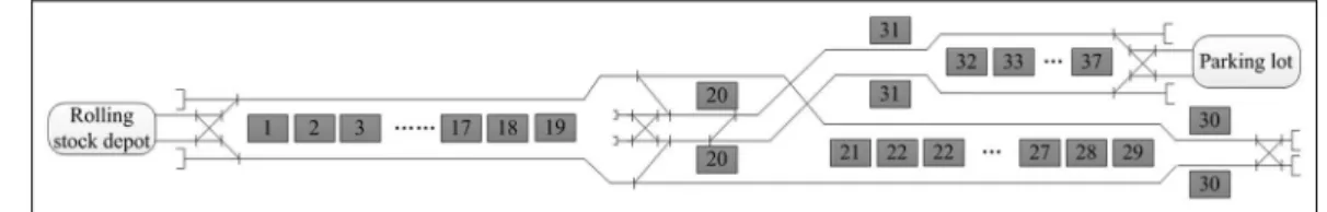
Figure 7 shows the layout of a Y-type urban rail transit line. The node station is L7, and b=20, m=10, and
n=7; there are 37 stations in total. Considering the modernization of the tracks, it was assumed that all the stations had turn-back tracks, so any station could be chosen as a turn-back location of a routing. The routings were assumed to adopt station-behind turn-back, so when Routinghturned back at stationk, the routing covered the station. Figure 8 shows passen-ger flow on each section in peak hour, and the research periodTis 7:30–8:30 a.m. in morning peak hour. The passenger volume was obtained from a pre-feasibility
Figure 6. Expression of chromosomes.
study of a line in China. According to the actual situa-tion of the line, the parameters adopted are shown in Table 4.
Result analysis
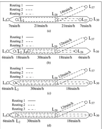
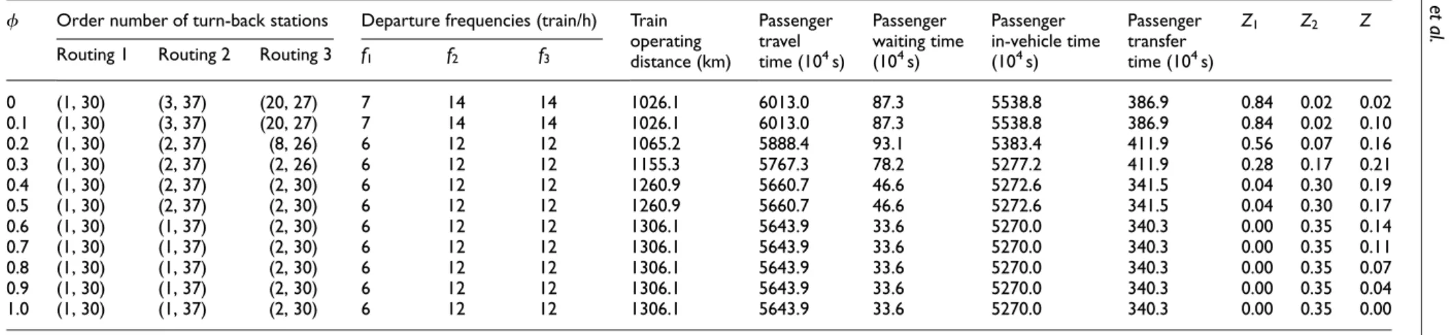
According to the proposed model, the weight value of the passenger travel time and the form of multi-routing planning affected the optimal solutions. Thus, this arti-cle calculated the optimal solutions under the form of three-routing and two-routing, respectively, with the weight increased from 0 to 1.0. The results are shown in Tables 5 and 6, and the forms of the routing plan-ning are shown in Figures 9 and 10.
Figure 9 shows that when the weight of the passen-ger travel time f increases, the passenger travel time decreases while the train operating distance increases. Whenfincreases from 0 to 0.2, the turn-back stations of Routing 2 and Routing 3 change to make the ings longer, and the departure frequencies of the rout-ings decrease to meet the constraint of the minimum track interval; when f increases from 0.3 to 1.0, the turn-back stations of Routing 2 and Routing 3 change to make both routings longer under the same departure frequencies, leading to less passenger travel time and more train operating distance.
Figure 10 shows that when the weight of the passen-ger travel time f increases from 0 to 0.4, Routing 2 becomes longer under the same departure frequencies, leading to less passenger travel time and more train operating distance; when f increases from 0.4 to 1.0,
Routing 2 becomes shorter to turn the straight-through operation to separate operation, so the frequencies of both routings could increase to 30 train/h which is the maximum frequency, leading to less passenger travel time and more train operating distance.
Comparison of three-routing planning and
two-routing planning
To discuss the influence of different routing planning and weight values on the objectives, passenger travel time (Z1) and train operating distance (Z2) of the
opti-mal solutions under the form of three-routing and two-routing planning with different weight values of passen-ger travelfare shown in Figure 11, respectively.
Figure 11 shows the following:
1. When the weight of the passenger travel time
increases, the passenger travel time of three-routing planning and two-three-routing planning
Table 4. Value of parameters.
Parameters nv Imin fmin h STmin STmax d to
Value 1860p 120 s 6 train/h 1.0 15 s 45 s 1.51 s 300 s
Figure 8. Passenger flow of each section in morning peak hour (7:30–8:30 a.m.).
Figure 9. Optimal solution of three-routing planning: (a)
0 (1, 30) (3, 37) (20, 27) 7 14 14 1026.1 6013.0 87.3 5538.8 386.9 0.84 0.02 0.02 0.1 (1, 30) (3, 37) (20, 27) 7 14 14 1026.1 6013.0 87.3 5538.8 386.9 0.84 0.02 0.10 0.2 (1, 30) (2, 37) (8, 26) 6 12 12 1065.2 5888.4 93.1 5383.4 411.9 0.56 0.07 0.16 0.3 (1, 30) (2, 37) (2, 26) 6 12 12 1155.3 5767.3 78.2 5277.2 411.9 0.28 0.17 0.21 0.4 (1, 30) (2, 37) (2, 30) 6 12 12 1260.9 5660.7 46.6 5272.6 341.5 0.04 0.30 0.19 0.5 (1, 30) (2, 37) (2, 30) 6 12 12 1260.9 5660.7 46.6 5272.6 341.5 0.04 0.30 0.17 0.6 (1, 30) (1, 37) (2, 30) 6 12 12 1306.1 5643.9 33.6 5270.0 340.3 0.00 0.35 0.14 0.7 (1, 30) (1, 37) (2, 30) 6 12 12 1306.1 5643.9 33.6 5270.0 340.3 0.00 0.35 0.11 0.8 (1, 30) (1, 37) (2, 30) 6 12 12 1306.1 5643.9 33.6 5270.0 340.3 0.00 0.35 0.07 0.9 (1, 30) (1, 37) (2, 30) 6 12 12 1306.1 5643.9 33.6 5270.0 340.3 0.00 0.35 0.04 1.0 (1, 30) (1, 37) (2, 30) 6 12 12 1306.1 5643.9 33.6 5270.0 340.3 0.00 0.35 0.00
Table 6. Optimal solutions of two-routing planning with different weight values.
f Turn-back stations Departure frequencies (train/h) Train operating distance (km)
Passenger travel time (104s)
Passenger waiting time (104s)
Passenger in-vehicle time (104s)
Passenger transfer time (104s)
Z1 Z2 Z
Routing 1 Routing 2 Routing 3 f1 f2 f3
0 (1, 30) (4, 37) – 12 12 – 1009.0 5972.1 41.1 5518.5 412.4 0.75 0.00 0.00 0.1 (1, 30) (3, 37) – 12 12 – 1009.0 5967.4 38.9 5517.0 411.6 0.74 0.00 0.07 0.2 (1, 30) (3, 37) – 12 12 – 1009.0 5967.4 38.9 5517.0 411.6 0.74 0.00 0.15 0.3 (1, 30) (3, 37) – 12 12 – 1009.0 5967.4 38.9 5517.0 411.6 0.74 0.00 0.22 0.4 (1, 30) (3, 37) – 12 12 – 1009.0 5967.4 38.9 5517.0 411.6 0.74 0.00 0.29 0.5 (1, 30) (20, 37) – 20 20 – 1233.3 5821.1 18.1 5333.6 469.4 0.40 0.27 0.33 0.6 (1, 30) (20, 37) – 20 20 – 1233.3 5821.1 18.1 5333.6 469.4 0.40 0.27 0.35 0.7 (1, 30) (20, 37) – 23 23 – 1418.3 5770.4 13.7 5304.8 452.0 0.29 0.49 0.35 0.8 (1, 30) (20, 37) – 28 28 – 1726.6 5714.4 9.2 5274.0 431.2 0.16 0.85 0.30 0.9 (1, 30) (20, 37) – 30 30 – 1850.0 5699.6 8.0 5266.7 424.8 0.13 1.00 0.21 1.0 (1, 30) (20, 37) – 30 30 – 1850.0 5699.6 8.0 5266.7 424.8 0.13 1.00 0.13
decreases, while the train operating distance increases.
2. When the weight of the passenger travel time
increases from 0.4 to 1.0, the operating
dis-tance of two-routing planning increases
sharply while the passenger travel time
decreases relatively flat. At the same time, the routing planning changes from Figure 9(b) to Figure 9(c), and the departure frequencies of both routings increase from 12 train/h to 20–30 train/h, leading to a quick increase in the train operating distance. However, the pas-senger flow of some stations on the line are relatively small because of the unbalanced characteristic, which makes the increase in the train operating distance more obvious than the decrease in the passenger travel time. Therefore, it is not necessary to increase the weight of the passengers too much because the cost increases much more.
3. When the weight of the passenger travel time
ranges from 0.7 to 0.8, both objectives of three-routing planning are better than two-three-routing planning. Routing 2 in the three-routing plan-ning does not cover L1–L2, so the passengers
aimed to the branch boarding at Station 1 need to transfer and the passenger walking time for transferring increased a little. However, the fre-quencies of L20–L30 and L20–L37 are 18 and
12 train/h in the three-routing planning and 15
and 15 train/h in the two-routing planning, respectively; as more passengers travel on the trunk line, the three-routing planning can decrease the waiting time for transferring, and the degree of decrease is larger than the degree of increase in the walking time mentioned previ-ously. Therefore, three-routing planning can better copy with the characteristics of the pas-sengers’ demand by increasing the departure fre-quencies on sections with larger passenger flow while decreasing departure frequencies on sec-tions with smaller passenger flow.
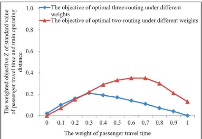
To discuss the influence of different routing planning and weight values on the comprehensive objective Zin formula (9), the comparison of Z under three-routing and two-routing with different weight values is shown in Figure 12. Zwas the weighted sum of the standard
value of the two objectives, so Z had no dimension,
and the range ofZwas [0, 1]. The values were obtained from Tables 5 and 6.
Figure 12 shows the following:
1. When the weight of the travel time increases,
the weighted objective of three-routing planning and two-routing both show decreasing trends after the first increase.
2. The smaller the weighted objective, the better the optimal solution. Thus, when f= 0.1–0.6, the optimal solution is a two-routing planning;
when f= 0.7–1.0, the optimal solution is a
three-routing planning. Therefore, three-routing planning is more suitable when the passenger travel time is more important while two-routing
Figure 10. Optimal solution of two-routing planning: (a)f=0, (b)f=0.1–0.4, and (c)f= 0.5–1.0.
planning is more suitable when the train operat-ing distance is more important.
Conclusion
In this study, a multi-routing planning design model of Y-type urban rail transit aimed at minimizing the pas-senger travel time and train operating distance was pro-posed, and the multi-objective model was turned into a single-objective model by giving the weight values of the objectives. The model optimized the departure fre-quencies and the locations of turn-backs of the routings considering the passenger demand and layout of the line. A GA was designed to obtain optimal solutions. A case was used to find out the effects of the variables on the objectives, and the standard values of the two objec-tives were given different weight values to discuss the change in routing planning. Also, the applicability of three-routing planning and two-routing planning was analyzed.
1. When the weight of the passenger travel time is lower, the optimal solution is two-routing plan-ning; when the weight is higher, the optimal solution is three-routing planning.
2. When the weight of the passenger travel time
increases, the passenger travel time of both three-routing planning and two-routing plan-ning decreases while the train operating distance of both increases.
3. When the weight of the passenger travel time
reaches to a certain value, three-routing plan-ning can better meet the unbalanced passenger flow than two-routing planning by increasing the departure frequencies on sections with large passenger demand while decreasing those with small passenger demand.
research.
Declaration of conflicting interests
The author(s) declared no potential conflicts of interest with respect to the research, authorship, and/or publication of this article.
Funding
The author(s) disclosed receipt of the following financial sup-port for the research, authorship, and/or publication of this article: This research was supported by National Natural Science Foundation of China (71390332) and National Natural Science Fund Projects (71571061, 71201007).
References
1. Vuchic VR. Urban transit: operation, planning and eco-nomics. Hoboken, NJ: John Wiley & Sons, Inc., 2004. 2. Furth PG. Short turning on transit routes. Transp Res
Record1987; 1108: 42–52.
3. Furth PG and Day FB. Transit routing and scheduling strategies for heavy demand corridors. Transp Res Record1985; 1011: 23–26.
4. Ceder A. Optimal design of transit short-turn trips. Transp Res Record1989; 1221: 8–22.
5. Ceder A and Stern HI. Deficit function bus scheduling with deadheading trip insertions for fleet size reduction. Transport Sci1981; 15: 338–363.
6. Nesheli MM and Ceder A. A robust, tactic-based, real-time framework for public-transport transfer synchroni-zation (The international symposium on transportation and traffic theory). Transp Res Procedia 2015; 9: 246–268.
7. Vijayaraghavan TAS and Anantharamaiah KM. Fleet assignment strategies in urban transportation using express and partial services.Transport Res A: Pol1995; 29: 157–171.
8. Corte´s CE, Jara-Dı´az S and Tirachini A. Integrating short turning and deadheading in the optimization of transit services. Transport Res A: Pol 2011; 45: 419–434.
9. Tirachini A, Corte´s CE and Jara-Dı´az S. Optimal design and benefits of a short turning strategy for a bus corri-dor.Transportation2011; 38: 169–189.
10. Site PD and Filippi F. Service optimization for bus corri-dors with short-turn strategies and variable vehicle size. Transport Res A: Pol1998; 32: 19–38.
11. Canca D, Barrena E, Laporte G, et al. A short-turning policy for the management of demand disruptions in rapid transit systems.Ann Oper Res. Epub ahead of print 3 July 2014. DOI: 10.1007/s10479-014-1663-x.
12. Jannson JO. A simple bus line model for optimization of service frequency and bus size. J Transp Econ Policy 1980; 14: 53–80.
13. Chen YJ, Yu JA, Zhou LS, et al. Study on the algorithm for train operation adjustment based on ordinal optimiza-tion.Adv Mech Eng2013; 5: 175347.
14. Riejos FAO, Barrena E, Ortiz JDC, et al. Analyzing the theoretical capacity of railway networks with a radial-backbone topology. Transport Res A: Pol 2015; 84: 83–92.
15. Xu R, Ma X and Song J. Study on operation plans of Shanghai Mingzhu transit system network.J Tongji Uni-vers2003; 31: 682–686 (in Chinese).
16. Fioole PJ, Kroon L, Maro´ti G, et al. A rolling stock cir-culation model for combining and splitting of passenger trains.Eur J Oper Res2006; 174: 1281–1297.
17. Freyss M, Giesen R and Mun˜oz JC. Continuous approxi-mation for skip-stop operation in rail transit.Transport Res C: Emer2013; 36: 419–433.