How does bias correction of regional climate model precipitation affect modelled runoff?

(1)

www.hydrol-earth-syst-sci.net/19/711/2015/ doi:10.5194/hess-19-711-2015

How does bias correction of regional climate model precipitation

affect modelled runoff?

J. Teng1, N. J. Potter1, F. H. S. Chiew1, L. Zhang1, B. Wang1, J. Vaze1, and J. P. Evans2 1_{CSIRO Land and Water Flagship, Canberra, Australia}

2_{Climate Change Research Centre and ARC Centre of Excellence for Climate System Science,}

University of New South Wales, Sydney, Australia

Correspondence to:J. Teng (jin.teng@csiro.au)

Received: 29 August 2014 – Published in Hydrol. Earth Syst. Sci. Discuss.: 23 September 2014 Revised: 11 December 2014 – Accepted: 8 January 2015 – Published: 4 February 2015

Abstract.Many studies bias correct daily precipitation from climate models to match the observed precipitation statistics, and the bias corrected data are then used for various mod-elling applications. This paper presents a review of recent methods used to bias correct precipitation from regional cli-mate models (RCMs). The paper then assesses four bias cor-rection methods applied to the weather research and forecast-ing (WRF) model simulated precipitation, and the follow-on impact on modelled runoff for eight catchments in south-east Australia. Overall, the best results are produced by ei-ther quantile mapping or a newly proposed two-state gamma distribution mapping method. However, the differences be-tween the methods are small in the modelling experiments here (and as reported in the literature), mainly due to the sub-stantial corrections required and inconsistent errors over time (non-stationarity). The errors in bias corrected precipitation are typically amplified in modelled runoff. The tested meth-ods cannot overcome limitations of the RCM in simulating precipitation sequence, which affects runoff generation. Re-sults further show that whereas bias correction does not seem to alter change signals in precipitation means, it can intro-duce additional uncertainty to change signals in high precip-itation amounts and, consequently, in runoff. Future climate change impact studies need to take this into account when deciding whether to use raw or bias corrected RCM results. Nevertheless, RCMs will continue to improve and will be-come increasingly useful for hydrological applications as the bias in RCM simulations reduces.

1 Introduction

Downscaling is a technique commonly used in hydrology when investigating the impact of climate change. It is a way of bridging the gap between low spatial resolution global cli-mate models (GCMs) and the regional-, catchment- or point-scale hydrological models (Fowler et al., 2007). Dynamical downscaling techniques derive regional-scale information by using a high-resolution climate model over a limited area and forcing it with lateral boundary conditions from GCMs or reanalysis products. In brief, it is modelling with a regional climate model, or RCM. With advances in RCMs and the in-creasing availability of RCM simulations, this type of down-scaling is gaining more and more popularity in hydrologi-cal impact studies (Dosio et al., 2012; Argüeso et al., 2013; Seaby et al., 2013; Teutschbein and Seibert, 2010; Maraun et al., 2010; Bennett et al., 2012). A drawback, however, is that precipitation simulations from RCMs are “biased”: in addition to errors inherited from the driving GCM, there are systematic RCM model errors, due to imperfect conceptu-alisation and parameterisation, inadequate length and qual-ity of reference data sets, and insufficient spatial resolution (Wilby et al., 2000; Wood et al., 2004; Piani et al., 2010b; Chen et al., 2011a; Christensen et al., 2008; Teutschbein and Seibert, 2010). Various “bias correction” methods have been developed in an attempt to minimise these errors (Boe et al., 2007; Piani et al., 2010a; Johnson and Sharma, 2012; Schmidli et al., 2006; Lenderink et al., 2007).

(2)

av-eraged over a certain area and time (Ehret et al., 2012); others have tried to distinguish model biases from model shortcom-ings and model errors (Teutschbein and Seibert, 2013). For clarity, in this paper we define bias as the systematic distor-tion of a statistical outcome from the expected value, and we use “error” or “difference” to refer to the discrepancy be-tween a model output and observations.

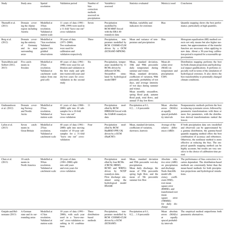
Many studies have compared and evaluated different bias correction methods; Table 1 summarises some recent ones and their main conclusions. Most of these studies investi-gated the impact of bias correction on precipitation and tem-perature (see column 6, Table 1), yet only Teutschbein and Seibert (2012) and Chen et al. (2013) tested the effect of bias correction on the outputs of hydrological models. Nearly all studies agree that distribution-based bias correction methods (both parametric and non-parametric) give the best perfor-mance in terms of reproducing the observed climate, whereas means-based methods, in particular linear scaling (LS), are almost always ranked as the least-skilled bias correction method.

Building on the knowledge gained from previous compar-ison studies, we have assessed in more detail the best per-forming bias correction technique – distribution mapping – and compared its performance in several forms against the linear scaling (LS) method as a benchmark (other names of the distribution mapping technique include quantile match-ing, distribution transformation, probability mappmatch-ing, and histogram equalisation). Our main interest is to examine the effect of bias correction on modelled runoff. The bias correc-tion methods were applied on modelled precipitacorrec-tion, as it is the most critical and difficult-to-model variable in hydrolog-ical studies (Vaze et al., 2011), and evaluated on both precip-itation and runoff using a cross-validation method. The raw and bias-corrected precipitation data were used to drive the hydrological models. The key precipitation and runoff char-acteristics were compared to those of observations to inves-tigate how bias correction affects RCM precipitation, and its follow-on impact on runoff propagating through hydrologi-cal models.

Previous studies have shown mixed results in ranking the different types of distribution mapping methods, suggesting that there may be only marginal differences between the methods. For example, some studies have shown that dis-tribution mapping based on theoretical disdis-tributions outper-forms other bias correction methods (Teutschbein and Seib-ert, 2013, 2012; Yang et al., 2010). Others have shown that theoretical distribution mapping performs similar to, or only marginally better than, empirical quantile mapping (Berg et al., 2012; Chen et al., 2013). Some studies, on the other hand, show that empirical quantile mapping demonstrates higher skill than theoretical distribution mapping in system-atically correcting RCM precipitation (Gudmundsson et al., 2012; Gutjahr and Heinemann, 2013; Li et al., 2010; La-fon, 2013). In view of the discrepancy in the literature, we compared three distribution mapping techniques, each with

increasing degree of dependency on the calibration data, in order to evaluate the methods based on both accuracy and robustness.

Berg et al. (2012) found that 30 years of calibration data are required to produce reasonable accuracy for the esti-mate of precipitation variance. Due to the difficult parame-terisation and expensive computational costs associated with RCMs, this requirement is not easily met in impact studies. In the main modelling experiments, we chose two 8-year-long periods of RCM data (16 years split in half), with signifi-cant climatic difference between them, to examine whether the bias correction method derived from one period works for another period, and if not, what causes it to fail. We then validated the generality of our conclusion using two 30-year-long RCM precipitation data sets (60 years split in half).

Chen et al. (2013) concluded that bias correction perfor-mance is location dependent and that virtually no bias cor-rection method succeeds in catchments having low coher-ence between RCM simulated and observed precipitation se-quences. We challenged (and confirmed) this conclusion by evaluating the precipitation sequence simulated by the RCM and quantifying the effect of precipitation sequence on mod-elled runoff.

The impact of bias correction on the change signals (one period vs. another) in both precipitation and runoff was also explored. There were two possible outcomes from this inves-tigation: if bias correction does not alter the change signals in the hydro-climatic projections, then the use of bias cor-rection should be considered either unnecessary or safe to use, depending on the circumstance (Muerth et al., 2013). If it does alter the change signal, bias correction could be re-ducing or increasing errors in the change signals, either way, it introduces an extra level of uncertainty in the modelling chain.

This paper contributes to the present lively discussion on whether bias correction methods should be applied to global and regional climate model data, a conversation ini-tiated by Christensen et al. (2008), stimulated by Ehret et al. (2012), and continued by more recent studies such as Muerth et al. (2013) and Teutschbein and Seibert (2013).

2 Study area and data

2.1 Study area

(3)

Table 1.Recent studies comparing different RCM bias correction methods. Study Study area Spatial

resolution

Validation period Number of bias correction methods assessed on precipitation

Variable(s) assessed

Statistics evaluated Metric(s) used Conclusion

Themeßl et al. (2011)

Domain cover-ing the Alpine region including Austria

Modelled at 10 km resolution. Validated at station scale

11 years of data (1981– 1990, 1999) were used in a 11-fold “leave one out” cross-validation

Seven Precipitation modelled by RCM MM5 forced with the ERA-40 reanalysis data

Median, variability and indicators for extremes

Bias Quantile mapping shows the best perfor-mance, particularly at high quantiles.

Berg et al. (2012)

Domain cover-ing the entirety of Germany and its near surrounding areas

Modelled at 7 km resolution. Validated against 1 km gridded observations

30 years of data (1971–2000). Two realisations were used for calibration and validation respectively

Three Precipitation, tem-perature modelled by RCM COSMO-CLM driven by a GCM (ECHAM5-MPIOM)

Mean and variance of tem-perature and precipitation

Bias Histogram equalisation (HE) method cor-rects not only means but also higher mo-ments, but approximations of the transfer function are necessary when applying to new data. About a 30-year-long calibra-tion period is required for a reasonable ap-proximation.

Teutschbein and Seibert (2012, 2013)

Five catch-ments in Sweden

Modelled at 25 km resolution. Validated at catchment scale (taken from one grid cell)

40 years of data (1961– 1990) were used for cal-ibration and validation in the first study and split into warm/cold years and dry/wet years for cross-validation in the second study

Six Precipitation, temper-ature modelled by 11 RCMs driven by different GCMs. Streamflow simu-lated by hydrological model HBV

Mean, standard deviation, 10th and 90th percentile daily temperature during summer and winter. Mean, standard deviation, coefficient of variation, 90th percentile, probability of wet days, and average intensity of wet days during summer and winter.

Mean monthly streamflow, spring flood peak, autumn flood peak, total flows, and annual 15 day low flows

Mean ab-solute error (MAE) on temperature and precipitation CDFs

Distribution mapping performs the best for both climate projections and hydrolog-ical impact qualifications. It performs es-pecially well in terms of the simulation of hydrological extremes. It also shows the best transferability to potentially changed climate conditions.

Gudmundsson et al. (2012)

Domain cover-ing Norway and Nordic Arctic

Modelled at 25 km resolution. Validated at station scale

41 years of data (1960– 2000) split into 10 sub-samples for a 10-fold “leave one out” cross-validation

11 Precipitation mod-elled by RCM HIRHAM forced with the EAR40 reanalysis data

Precipitation at 0.1, 0.2,. . . 1.0 percentile

Mean absolute errors (MAEs) at equally spaced probabil-ity intervals

Nonparametric methods perform the best in reducing systematic errors, followed by parametric transformations with three or more free parameters, with the distribu-tion derived transformadistribu-tions ranked the lowest.

Lafon et al. (2013)

Seven catch-ments in Great Britain

Modelled at 25 km resolution. Validated at catchment scale

40 years of data (1961– 2000) split into moving window of 10-year sub-samples for a 31-fold “leave one out” cross-validation

Four Precipitation mod-elled by RCM HadRM3-PPE-UK driven by a GCM (HadCM3)

Mean, standard deviation, coefficient of variation, skewness, kurtosis

Average of the relative differ-ences (ARD)

If both precipitation data sets (modelled and observed) can be approximated by a gamma distribution, the gamma-based quantile mapping method offers the best combination of accuracy and robustness. Otherwise, the nonlinear method is more effective at reducing the bias. The em-pirical quantile mapping method can be highly accurate, but results are very sen-sitive to the choice of calibration time pe-riod.

Chen et al. (2013)

10 catch-ments in North America

Modelled at 50 km resolution. Validated at catchment scale

20 years of data (1981–2000) split into odd years and even years for cross-validation

Six Precipitation mod-elled by four RCMs (CRCM, HRM3, RCM3 and WRFG) driven by NCEP reanalysis data. Flow discharge sim-ulated using the hydrological model HSAMI

Mean, standard deviation and 95th percentile wet-day precipitation.

Mean daily discharge, the mean of 95th percentile spring high flow, and the mean of 5th percentile summer low flow

Absolute rela-tive error (ARE) on precipitation and discharge Nash–Sutcliffe model effi-ciency coeffi-cient (NSE), root mean square error (RMSE), and transformed root mean square error (TRMSE) for daily dis-charge

The performance of bias correction is lo-cation dependent. The distribution-based methods are consistently better than the mean-based methods for both precipita-tion projecprecipita-tions and hydrological simula-tions.

Gutjahr and Hel-nemann (2013)

A German state and its sur-rounding areas

Modelled at 4.5 km resolution. Validated at station scale

10 years of data (1991– 2000), with each year used in a “leave-one-out” cross-validation re-sulting in 81 combina-tions

Three distribution-based methods

Precipitation, tem-perature modelled by RCM COSMO-CLM driven by a GCM (ECHAM5)

Precipitation at 0.1, 0.2,. . . 1.0 percentile

Mean absolute errors (MAEs) at equally spaced probabil-ity intervals

The empirical method outperforms both parametric alternatives.

basins, with areas from 250 to 1033 km2, were selected for this study. The catchments were mostly unregulated, with continuous climate and streamflow measurements available for 1985–2000, as such the assessment period was chosen. An 8-year period unaffected by the drought (1985–1992) was used as the calibration period, and another 8-year pe-riod strongly affected by the drought (1993–2000) was used

as the validation period. Subsequently, they were switched for cross-validation. The observations and RCM simulations are aggregated to each catchment and compared at this level.

2.1.1 Observations

(4)

405240 406224

405217 405228

407222

406213

405226

407215

L O D D O N R I V E R L O D D O N R I V E R

G O U L B U R N R I V E R G O U L B U R N R I V E R

Y A R R A R I V E R Y A R R A R I V E R C A M P A S P E R I V E R

C A M P A S P E R I V E R

B A R W O N R I V E R B A R W O N R I V E R

B U N Y I P R I V E R B U N Y I P R I V E R M O O R A B O O L R I V E R

M O O R A B O O L R I V E R W E R R I B E E R I V E R W E R R I B E E R I V E R

B R O K E N R I V E R B R O K E N R I V E R

L A K E C O R A N G A M I T E L A K E C O R A N G A M I T E

M A R I B Y R N O N G R I V E R M A R I B Y R N O N G R I V E R A V O C A R I V E R

A V O C A R I V E R

H O P K I N S R I V E R H O P K I N S R I V E R

M U R R A Y - R I V E R I N A M U R R A Y - R I V E R I N A

L A T R O B E R I V E R L A T R O B E R I V E R

O T W A Y C O A S T O T W A Y C O A S T

145° E 145° E

144° E 144° E

3

7

°

S

3

7

°

S

3

8

°

S

3

8

°

S

Legend

Study catchments

AWRC river basins

.

0 12.5 25 50 75 100

Kilometers

D

D E

E

Figure 1.Map showing the eight study catchments (white with red outline, large map), and their locations within the major river basins devised by the Australian Water Resources Council (AWRC). The unique symbols in each catchment identify the catchments and will be used in later figures.

catchment. The source of this data set was the SILO Data Drill (http://www.longpaddock.qld.gov.au/silo) of the De-partment of Science, Information Technology, Innovation and the Arts, Queensland, Australia (Jeffrey et al., 2001). The SILO gridded climate data sets provide surfaces of daily rainfall and other climate data interpolated from high quality point measurements provided by the Australian Bureau of Meteorology. The daily potential evapotranspiration (PET) sequences used in the hydrological modelling were calcu-lated from SILO climate variables using Morton’s wet en-vironment algorithms (Chiew and McMahon, 1991). Mea-sured daily streamflow data were sourced from a previous study (Vaze et al., 2010) and used to calibrate the hydrologi-cal models.

2.1.2 RCM data

Most of the analysis in this study was carried out using daily precipitation series for the period 1985–2000, which were simulated by Evans and McCabe (2010) using the weather research and forecasting (WRF) model. Another 60-year-long (1950–2009) WRF precipitation data set (Evans et al.,

2014) was used to validate the conclusion reached by us-ing the shorter data set. For both data sets, WRF was im-plemented on a 10 km grid using lateral boundary condi-tions taken from the National Centers for Environmental Pre-diction (NCEP)/National Center for Atmospheric Research (NCAR) reanalysis data set (Kalnay et al., 1996, see http: //www.cdc.noaa.gov/cdc/reanalysis). The WRF simulations have been found capable of capturing the drought experi-enced over the study area in another study (Evans and Mc-Cabe, 2010). The daily precipitation series for each catch-ment were aggregated from the WRF simulation by averag-ing all the grid cells over the catchment.

3 Method

3.1 Bias correction methods

In this study, daily precipitation was the main variable sub-jected to bias correction. Typically, bias correction methods aim to correct the mean, variance and/or distribution of the modelled precipitation by using a functionh:

ˆ

pobs=h(pmod) (1)

so that the transformed precipitation matches the observed data more closely than the modelled precipitation.

3.1.1 Linear scaling (LS)

The simplest choice forhis probably a linear transformation

ˆ

pobs=apmod, (2)

wherea is a free parameter that is subject to calibration. This simple form of bias correction is widely used to ad-just precipitation from GCMs, RCMs and statistical down-scaling methods (Maraun et al., 2010; Teng et al., 2012a). It can efficiently correct the means but does not account for the higher moments. In this study, this method served as the benchmark as LS has been identified in various studies as the least skilful bias correction method (Gudmundsson et al., 2012; Lafon, 2013; Chen et al., 2013; Teutschbein and Seib-ert, 2012). The LS parametera was optimised for each sea-son: DJF (December–February), MAM (March–May), JJA (June–August) and SON (September–November) to account for precipitation seasonality. Similarly, seasonal optimisation was also applied for all the other bias correction methods used in this study.

3.1.2 Distribution mapping using the gamma

distribution (DMG)

The relation in Eq. (1) can also be modelled so that the dis-tribution of the modelled precipitation matches that of the observations:

ˆ

(5)

0

10

20

30

405240 RCM JJA (1985−1992)

Probability(%)

Daily precipitation (mm)

99.8 99.5 99.0 98.0 95.0 90.0 80.0 50.0 ECDF

Gamma( α =0.35, β =0.17) Double Gamma( λ =0.41)

Double Gamma1( α =0.51, β =0.11) Double Gamma2( α =0.53, β =1.47)

Figure 2. CDF plot comparing a gamma distribution (red) and a double gamma distribution (green), which consists of two gamma distributions (blue and yellow) fitted to the same precipitation data for one study catchment. The empirical distribution is shown in black.

whereFmodis the cumulative distribution function (CDF) of

Pmod and Fobs−1 is the inverse CDF corresponding to Pobs.

These CDFs can either be theoretical distributions fitted to the data, or empirical distributions estimated by sorting the data. The gamma distribution with shape parameter α and rate parameterβ(Eq. 4) is often used to represent non-zero precipitation amounts (Piani et al., 2010a; Lafon, 2013), as it has the ability to approximate the positively skewed distri-butions (Yang et al., 2010). The probability density function (PDF) for a gamma random variable is given by:

f (p)=β

α_pα−1_e−βp

Ŵ(α) , (4)

whereŴ(α)is the gamma function evaluated atα.

When estimating parameters for the gamma distribution, we used the method of maximum-likelihood estimation as it is more accurate (i.e. the standard error of the estimates is lower) compared to the method of moments or least-squares estimation (e.g. Piani et al., 2010a).

Given an occurrence of non-zero precipitation amount

pi>0 for i=1, . . ., n, the log-likelihood function of the

gamma distribution can be written as:

l(α, β)=

n X

i=1

logf (pi;α, β). (5)

The maximum-likelihood estimates forαandβ are chosen to maximise this log-likelihood function. To account for dry days, we define the PDF for zero and non-zero precipitation

daysf0(p)as a mixed distribution with an atom of

probabil-ity atp=0 and a gamma distribution forp >0 so that:

f0(p)= (

q0, p=0

(1−q0)βαpα−1e−βp

Ŵ(α) , p >0.

(6)

The maximum likelihood estimate ofq0depends only on the

relative number of zero-precipitation days (n0):

q0=n0/n. (7)

The shape and rate parametersαandβare calculated on the non-zero precipitation amounts.

3.1.3 Distribution mapping using a double gamma

distribution (DM2G)

Daily precipitation distributions are typically heavily skewed towards high-intensity values. As a result, when fitting a sin-gle gamma distribution, the distribution parameters will be dictated by the most frequently occurring values, but may then not accurately represent the extremes. To capture normal precipitation values as well as extremes, different approaches have been tried, but the most common is to divide the pre-cipitation distribution into segments and fit separate distri-butions to each segment (Yang et al., 2010; Grillakis et al., 2013; Gutjahr and Heinemann, 2013; Smith et al., 2014). In-stead of introducing arbitrary cut-offs, we propose what can be interpreted as a two-state distribution. It is a mix of two gamma distributions which can model non-zero precipitation amounts:

f (p)=λβ

α1

1 p

α1−1_e−β1p

Ŵ(α1)

+(1−λ)β

α2

2 p

α2−1_e−β2p

Ŵ(α2)

(8)

with 0< λ <1. The parameterλis the relative occurrence of the states, and, fitted correctly, the two gamma distributions represent rainfall occurring in high and low rainfall states. The advantage of this approach compared to segmenting the distribution is that all parameters can be estimated simulta-neously using maximum-likelihood estimation. Thus, six pa-rameters –q0,α1,β1,α2,β2 andλ– were estimated from

observations and from the RCM output for the calibration period; they were then used to correct the RCM output for the validation period.

(6)

RCM RCM −40 −20 0 20 40 Annual precipitation Relativ

e bias (%)

LS_same LS_same −40 −20 0 20 40 LS_cross LS_cross −40 −20 0 20 40 DMG_same DMG_same −40 −20 0 20 40 DMG_cross DMG_cross −40 −20 0 20 40 DM2G_same DM2G_same −40 −20 0 20 40 DM2G_cross DM2G_cross −40 −20 0 20 40 QM_same QM_same −40 −20 0 20 40 QM_cross QM_cross −40 −20 0 20 40 1985−1992 1993−2000 RCM RCM −40 −20 0 20 40 DJF precipitation Relativ

e bias (%)

LS_same LS_same −40 −20 0 20 40 LS_cross LS_cross −40 −20 0 20 40 DMG_same DMG_same −40 −20 0 20 40 DMG_cross DMG_cross −40 −20 0 20 40 DM2G_same DM2G_same −40 −20 0 20 40 DM2G_cross DM2G_cross −40 −20 0 20 40 QM_same QM_same −40 −20 0 20 40 QM_cross QM_cross −40 −20 0 20 40 1985−1992 1993−2000 RCM RCM −40 −20 0 20 40 MAM precipitation Relativ

e bias (%)

LS_same LS_same −40 −20 0 20 40 LS_cross LS_cross −40 −20 0 20 40 DMG_same DMG_same −40 −20 0 20 40 DMG_cross DMG_cross −40 −20 0 20 40 DM2G_same DM2G_same −40 −20 0 20 40 DM2G_cross DM2G_cross −40 −20 0 20 40 QM_same QM_same −40 −20 0 20 40 QM_cross QM_cross −40 −20 0 20 40 1985−1992 1993−2000 RCM RCM −40 −20 0 20 40 JJA precipitation Relativ

e bias (%)

LS_same LS_same −40 −20 0 20 40 LS_cross LS_cross −40 −20 0 20 40 DMG_same DMG_same −40 −20 0 20 40 DMG_cross DMG_cross −40 −20 0 20 40 DM2G_same DM2G_same −40 −20 0 20 40 DM2G_cross DM2G_cross −40 −20 0 20 40 QM_same QM_same −40 −20 0 20 40 QM_cross QM_cross −40 −20 0 20 40 1985−1992 1993−2000 RCM RCM −40 −20 0 20 40 SON precipitation Relativ

e bias (%)

LS_same LS_same −40 −20 0 20 40 LS_cross LS_cross −40 −20 0 20 40 DMG_same DMG_same −40 −20 0 20 40 DMG_cross DMG_cross −40 −20 0 20 40 DM2G_same DM2G_same −40 −20 0 20 40 DM2G_cross DM2G_cross −40 −20 0 20 40 QM_same QM_same −40 −20 0 20 40 QM_cross QM_cross −40 −20 0 20 40 1985−1992 1993−2000 RCM RCM −40 −20 0 20 40

99th percentile precipitation

Relativ

e bias (%)

99th percentile 3−day cumulative pr.

Relativ

e bias (%)

Relativ

e bias (%)

Dry days per year

Bias (da ys) LS_same LS_same −40 −20 0 20 40 LS_cross LS_cross −40 −20 0 20 40 DMG_same DMG_same −40 −20 0 20 40 DMG_cross DMG_cross −40 −20 0 20 40 DM2G_same DM2G_same −40 −20 0 20 40 DM2G_cross DM2G_cross −40 −20 0 20 40 QM_same QM_same −40 −20 0 20 40 QM_cross QM_cross −40 −20 0 20 40 1985−1992 1993−2000

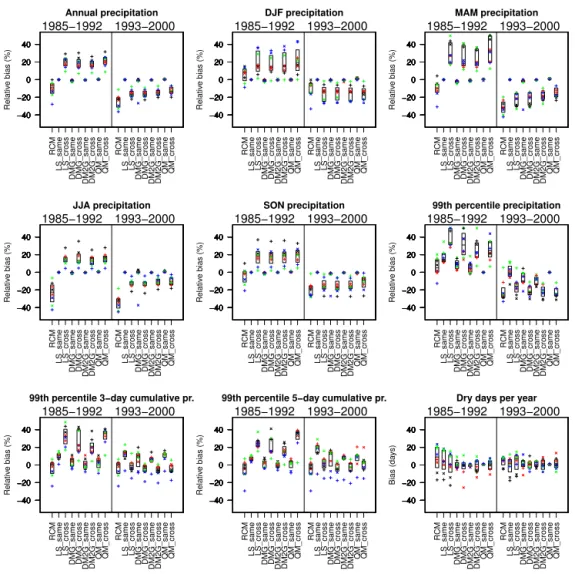
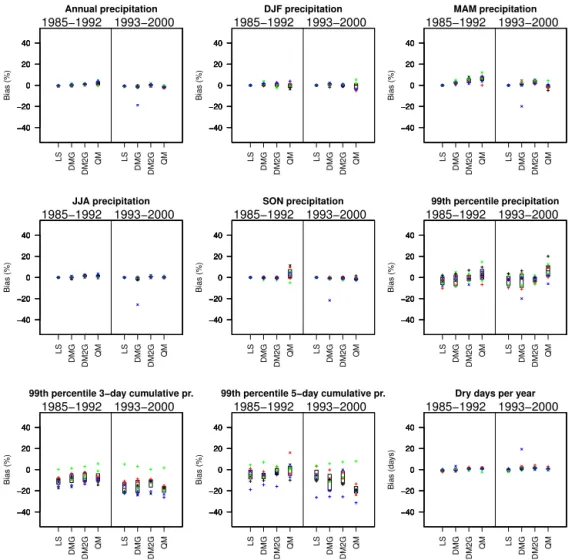
Figure 3.Relative bias of precipitation characteristics, expressed as percentage differences relative to observations between raw RCM and bias corrected RCM precipitation. Each panel displays a different characteristic (title at top of panel) and the percentages were calculated after applying four different bias correction methods (key at bottom) to eight catchments over two periods (1985–1992, left; 1993–2000, right). The bias correction methods were LS, DMG, DM2G and QM (see text), the “_same” suffix denotes calibration and the “_cross” refers to cross-validation. Boxes indicate interquartile range; markers indicate the numbers from each catchment (markers are constrained to the edges of the plotting area if the values exceed the range of plotting); the symbol for each catchment can be found in Fig. 1.

3.1.4 Empirical quantile mapping (QM)

Apart from using theoretical distributions, the empirical CDF is also commonly used to solve Eq. (3) (Themeßl et al., 2011; Gudmundsson et al., 2012; Boe et al., 2007; Bennett et al., 2014). Here the empirical CDFs of observed and modelled precipitation were estimated using empirical percentiles. Val-ues in between the percentiles were approximated using lin-ear interpolation. In cases where new RCM values (such as from the validation period) were larger than the calibration values used to estimate the empirical CDF, a linear regres-sion fit on the last five data points was used to extrapolate be-yond the range of observations and allow for possible “new extremes”.

3.2 Hydrological modelling (HM)

(7)

RCM RCM −100 −50 0 50 100 150 200 Annual runoff Relativ

e bias (%)

LS_same LS_same −100 −50 0 50 100 150 200 LS_cross LS_cross −100 −50 0 50 100 150 200 DMG_same DMG_same −100 −50 0 50 100 150 200 DMG_cross DMG_cross −100 −50 0 50 100 150 200 DM2G_same DM2G_same −100 −50 0 50 100 150 200 DM2G_cross DM2G_cross −100 −50 0 50 100 150 200 QM_same QM_same −100 −50 0 50 100 150 200 QM_cross QM_cross −100 −50 0 50 100 150 200 HM_calib HM_calib −100 −50 0 50 100 150 200 HM_cross HM_cross −100 −50 0 50 100 150

200 1985−1992 1993−2000

RCM RCM −100 −50 0 50 100 150 200 DJF runoff Relativ

e bias (%)

200 1985−1992 1993−2000

RCM RCM −100 −50 0 50 100 150 200 MAM runoff Relativ

e bias (%)

200 1985−1992 1993−2000

RCM RCM −100 −50 0 50 100 150 200 JJA runoff Relativ

e bias (%)

200 1985−1992 1993−2000

RCM RCM −100 −50 0 50 100 150 200 SON runoff Relativ

e bias (%)

200 1985−1992 1993−2000

RCM RCM −100 −50 0 50 100 150 200

99th percentile runoff

Relativ

e bias (%)

200 1985−1992 1993−2000

RCM RCM −100 −50 0 50 100 150 200

Low runoff days per year

Bias (da ys) LS_same LS_same −100 −50 0 50 100 150 200 LS_cross LS_cross −100 −50 0 50 100 150 200 DMG_same DMG_same −100 −50 0 50 100 150 200 DMG_cross DMG_cross −100 −50 0 50 100 150 200 DM2G_same DM2G_same −100 −50 0 50 100 150 200 DM2G_cross DM2G_cross −100 −50 0 50 100 150 200 QM_same QM_same −100 −50 0 50 100 150 200 QM_cross QM_cross −100 −50 0 50 100 150 200 HM_calib HM_calib −100 −50 0 50 100 150 200 HM_cross HM_cross −100 −50 0 50 100 150

200 1985−1992 1993−2000

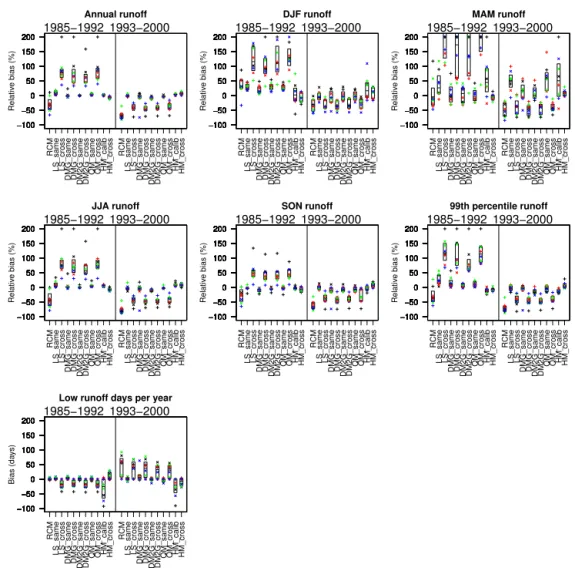
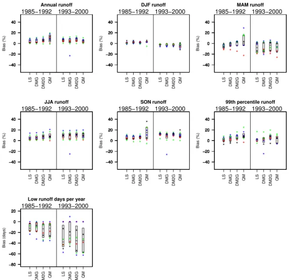
Figure 4.Relative bias in runoff characteristics derived from precipitation-driven hydrological model GR4J. Values are percentage differ-ences, relative to runoff modelled from observed precipitation, when GR4J was driven by raw RCM precipitation and bias corrected RCM precipitation. Same layout as Fig. 3, with additional HM_calib and HM_cross, which represent calibration errors and cross-validation errors from GR4J alone.

model parameters optimised to maximise the NSE-bias ob-jective function; this function is a weighted combination of the Nash–Sutcliffe efficiency (Nash and Sutcliffe, 1970) and a logarithmic function of bias in the modelled mean annual streamflow (Viney et al., 2009). The models were run at a daily time step. To estimate the impact of bias correction on runoff, the models were driven by WRF precipitation be-fore and after bias correction using the optimised parameters derived from the calibrations described above. The same PET data set calculated using observed climate variables was used throughout the hydrological modelling. By keeping PET the same, the possible impact of PET and the correlation between RCM precipitation and PET was not considered in this study to isolate the impact of precipitation.

3.3 Evaluating performance

(8)

RCM RCM −100 −50 0 50 100 150 200 Annual runoff Relativ

e bias (%)

200 1985−1992 1993−2000

RCM RCM −100 −50 0 50 100 150 200 DJF runoff Relativ

e bias (%)

200 1985−1992 1993−2000

RCM RCM −100 −50 0 50 100 150 200 MAM runoff Relativ

e bias (%)

200 1985−1992 1993−2000

RCM RCM −100 −50 0 50 100 150 200 JJA runoff Relativ

e bias (%)

200 1985−1992 1993−2000

RCM RCM −100 −50 0 50 100 150 200 SON runoff Relativ

e bias (%)

200 1985−1992 1993−2000

RCM RCM −100 −50 0 50 100 150 200

Relativ

e bias (%)

200 1985−1992 1993−2000

RCM RCM −100 −50 0 50 100 150 200

Bias (da ys) LS_same LS_same −100 −50 0 50 100 150 200 LS_cross LS_cross −100 −50 0 50 100 150 200 DMG_same DMG_same −100 −50 0 50 100 150 200 DMG_cross DMG_cross −100 −50 0 50 100 150 200 DM2G_same DM2G_same −100 −50 0 50 100 150 200 DM2G_cross DM2G_cross −100 −50 0 50 100 150 200 QM_same QM_same −100 −50 0 50 100 150 200 QM_cross QM_cross −100 −50 0 50 100 150 200 HM_calib HM_calib −100 −50 0 50 100 150 200 HM_cross HM_cross −100 −50 0 50 100 150

200 1985−1992 1993−2000

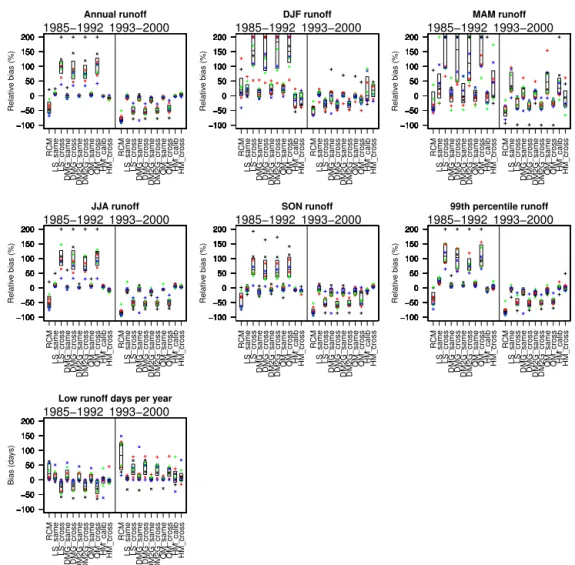
Figure 5.As for Fig. 4, but using results from hydrological model Sacramento.

To gauge the impact of bias correction methods on precip-itation, we compared the RCM precipitation before and after bias correction with the observations using salient metrics: annual and seasonal means, 99th percentile precipitation as an indicator of high precipitation events, number of dry days (daily precipitation less than 0.1 mm) per year as an indica-tor of low precipitation, and 99th percentile of 3- and 5-day cumulative precipitation as indicators of runoff-generating events. The runoff modelled using RCM precipitation be-fore and after bias correction was also evaluated against key runoff characteristics: annual and seasonal means, 99th per-centile runoff as an indicator of high-flow events, and number of low-flow days (daily runoff less than 0.01 mm) as an in-dicator of low-flow conditions. We also looked at the effect of bias correction methods on change signals by comparing the relative difference in precipitation and runoff between the two periods derived from various methods.

4 Results

(9)

RCM RCM

−40 −20 0 20 40

Annual precipitation

Bias (%)

LS LS

−40 −20 0 20 40

DMG DMG

−40 −20 0 20 40

DM2G DM2G

−40 −20 0 20 40

QM QM

−40 −20 0 20 40

1985−1992 1993−2000

RCM RCM

−40 −20 0 20 40

DJF precipitation

Bias (%)

LS LS

−40 −20 0 20 40

DMG DMG

−40 −20 0 20 40

DM2G DM2G

−40 −20 0 20 40

QM QM

−40 −20 0 20 40

1985−1992 1993−2000

RCM RCM

−40 −20 0 20 40

MAM precipitation

Bias (%)

LS LS

−40 −20 0 20 40

DMG DMG

−40 −20 0 20 40

DM2G DM2G

−40 −20 0 20 40

QM QM

−40 −20 0 20 40

1985−1992 1993−2000

RCM RCM

−40 −20 0 20 40

JJA precipitation

Bias (%)

LS LS

−40 −20 0 20 40

DMG DMG

−40 −20 0 20 40

DM2G DM2G

−40 −20 0 20 40

QM QM

−40 −20 0 20 40

1985−1992 1993−2000

RCM RCM

−40 −20 0 20 40

SON precipitation

Bias (%)

LS LS

−40 −20 0 20 40

DMG DMG

−40 −20 0 20 40

DM2G DM2G

−40 −20 0 20 40

QM QM

−40 −20 0 20 40

1985−1992 1993−2000

RCM RCM

−40 −20 0 20 40

Bias (%)

LS LS

−40 −20 0 20 40

DMG DMG

−40 −20 0 20 40

DM2G DM2G

−40 −20 0 20 40

QM QM

−40 −20 0 20 40

1985−1992 1993−2000

RCM RCM

−40 −20 0 20 40

Bias (%)

LS LS

−40 −20 0 20 40

DMG DMG

−40 −20 0 20 40

DM2G DM2G

−40 −20 0 20 40

QM QM

−40 −20 0 20 40

1985−1992 1993−2000

RCM RCM

−40 −20 0 20 40

Bias (%)

LS LS

−40 −20 0 20 40

DMG DMG

−40 −20 0 20 40

DM2G DM2G

−40 −20 0 20 40

QM QM

−40 −20 0 20 40

1985−1992 1993−2000

RCM RCM

−40 −20 0 20 40

Bias (da

ys)

LS LS

−40 −20 0 20 40

DMG DMG

−40 −20 0 20 40

DM2G DM2G

−40 −20 0 20 40

QM QM

−40 −20 0 20 40

1985−1992 1993−2000

Figure 6.Differences between RCM simulations and observations in change signals in precipitation characteristics between periods 1985– 1992 and 1993–2000. The left and right panels indicate the validation periods in each case.

4.1 Impact on precipitation

The calibration results in Fig. 3 (denoted by “_same”) show that, as expected, all the bias correction methods are able to match the annual and seasonal means of precipitation when validating on the same period as the calibration period (see LS_same, DMG_same, DM2G_same and QM_same in the boxplots of annual and seasonal means in Fig. 3). For in-stance, LS perfectly corrects the median errors in annual means for the two periods (0 and 0 %), followed by DM2G (−0.3 and −0.2 %), QM (0.4 and 0.6 %) and DMG (−0.7 and−0.7 %). Only the distribution mapping methods (DMG, DM2G and QM) are able to reduce the errors in the high- and low-precipitation characteristics; QM in particular performs exceptionally well in reproducing 99th percentile precipita-tion and number of dry days per year. LS is not only unable to reduce the errors in high- and low-precipitation character-istics, but also increases the errors in some cases, as seen in the 99th percentile precipitation for 1985–1992 (period I, left panels) and number of dry days per year for 1993–2000

(pe-riod II, right panels). This is consistent with the findings from previous studies (Chen et al., 2013; Teutschbein and Seibert, 2012).

(10)

precipi-LS LS

−40 −20 0 20 40

Annual precipitation

Bias (%)

DMG DMG

−40 −20 0 20 40

DM2G DM2G

−40 −20 0 20 40

QM QM

−40 −20 0 20 40

1985−1992 1993−2000

LS LS

−40 −20 0 20 40

DJF precipitation

Bias (%)

DMG DMG

−40 −20 0 20 40

DM2G DM2G

−40 −20 0 20 40

QM QM

−40 −20 0 20 40

1985−1992 1993−2000

LS LS

−40 −20 0 20 40

MAM precipitation

Bias (%)

DMG DMG

−40 −20 0 20 40

DM2G DM2G

−40 −20 0 20 40

QM QM

−40 −20 0 20 40

1985−1992 1993−2000

LS LS

−40 −20 0 20 40

JJA precipitation

Bias (%)

DMG DMG

−40 −20 0 20 40

DM2G DM2G

−40 −20 0 20 40

QM QM

−40 −20 0 20 40

1985−1992 1993−2000

LS LS

−40 −20 0 20 40

SON precipitation

Bias (%)

DMG DMG

−40 −20 0 20 40

DM2G DM2G

−40 −20 0 20 40

QM QM

−40 −20 0 20 40

1985−1992 1993−2000

LS LS

−40 −20 0 20 40

Bias (%)

DMG DMG

−40 −20 0 20 40

DM2G DM2G

−40 −20 0 20 40

QM QM

−40 −20 0 20 40

1985−1992 1993−2000

LS LS

−40 −20 0 20 40

Bias (%)

DMG DMG

−40 −20 0 20 40

DM2G DM2G

−40 −20 0 20 40

QM QM

−40 −20 0 20 40

1985−1992 1993−2000

LS LS

−40 −20 0 20 40

Bias (%)

DMG DMG

−40 −20 0 20 40

DM2G DM2G

−40 −20 0 20 40

QM QM

−40 −20 0 20 40

1985−1992 1993−2000

LS LS

−40 −20 0 20 40

Bias (da

ys)

DMG DMG

−40 −20 0 20 40

DM2G DM2G

−40 −20 0 20 40

QM QM

−40 −20 0 20 40

1985−1992 1993−2000

Figure 7.Differences between bias-corrected RCM and raw RCM simulations in change signals in precipitation characteristics between the periods 1985–1992 and 1993–2000. The left and right panels indicate the validation periods in each case.

tation, with more than 60 % of the precipitation coming from JJA and SON.

4.2 Impact on runoff

Figure 4 presents the relative differences in runoff character-istics simulated by GR4J using raw RCM and bias corrected precipitation when compared to those modelled using ob-served precipitation. The layout is similar to Fig. 3 except, for perspective, two boxes are added to each panel to show the conventional hydrological model errors: “HM_calib”, which represents the calibration error (when runoff from GR4J driven by observed precipitation is compared with observed streamflow); and “HM_cross”, which represents the cross-validation error (when GR4J runoff driven by observed pre-cipitation and using parameters calibrated to the same period is compared with those using parameters calibrated to a dif-ferent period).

The errors in runoff show a similar pattern to those for precipitation, but are much larger. They are also

consider-ably larger than the hydrological model errors. For instance, the median errors in mean annual runoff simulated using raw RCM precipitation increase to−33.1 % (period I) and

−69.5 % (period II). The calibration results show that LS is no longer able to correct the errors in annual and seasonal mean runoff to zero due to errors in high-percentile precipita-tion (see the 99th percentile precipitaprecipita-tion plot in Fig. 3) and, consequently, in high runoff. QM does not perform very well in correcting the high- and low-runoff characteristics as it was able to do for the high- and low-precipitation character-istics which may relate to its weakness (as shown in Fig. 3) in reproducing 3-day and 5-day cumulative precipitation. These results highlight the importance of precipitation sequence in runoff production, as discussed in Sect. 5.3.

(11)

RCM RCM

−60 −40 −20 0 20 40

Annual runoff

Bias (%)

LS LS

−60 −40 −20 0 20 40

DMG DMG

−60 −40 −20 0 20 40

DM2G DM2G

−60 −40 −20 0 20 40

QM QM

−60 −40 −20 0 20 40

HM_calib HM_calib

−60 −40 −20 0 20 40

HM_cross HM_cross

−60 −40 −20 0 20 40

1985−1992 1993−2000

RCM RCM

−60 −40 −20 0 20 40

DJF runoff

Bias (%)

LS LS

−60 −40 −20 0 20 40

DMG DMG

−60 −40 −20 0 20 40

DM2G DM2G

−60 −40 −20 0 20 40

QM QM

−60 −40 −20 0 20 40

HM_calib HM_calib

−60 −40 −20 0 20 40

HM_cross HM_cross

−60 −40 −20 0 20 40

1985−1992 1993−2000

RCM RCM

−60 −40 −20 0 20 40

MAM runoff

Bias (%)

LS LS

−60 −40 −20 0 20 40

DMG DMG

−60 −40 −20 0 20 40

DM2G DM2G

−60 −40 −20 0 20 40

QM QM

−60 −40 −20 0 20 40

HM_calib HM_calib

−60 −40 −20 0 20 40

HM_cross HM_cross

−60 −40 −20 0 20 40

1985−1992 1993−2000

RCM RCM

−60 −40 −20 0 20 40

JJA runoff

Bias (%)

LS LS

−60 −40 −20 0 20 40

DMG DMG

−60 −40 −20 0 20 40

DM2G DM2G

−60 −40 −20 0 20 40

QM QM

−60 −40 −20 0 20 40

HM_calib HM_calib

−60 −40 −20 0 20 40

HM_cross HM_cross

−60 −40 −20 0 20 40

1985−1992 1993−2000

RCM RCM

−60 −40 −20 0 20 40

SON runoff

Bias (%)

LS LS

−60 −40 −20 0 20 40

DMG DMG

−60 −40 −20 0 20 40

DM2G DM2G

−60 −40 −20 0 20 40

QM QM

−60 −40 −20 0 20 40

HM_calib HM_calib

−60 −40 −20 0 20 40

HM_cross HM_cross

−60 −40 −20 0 20 40

1985−1992 1993−2000

RCM RCM

−60 −40 −20 0 20 40

Bias (%)

LS LS

−60 −40 −20 0 20 40

DMG DMG

−60 −40 −20 0 20 40

DM2G DM2G

−60 −40 −20 0 20 40

QM QM

−60 −40 −20 0 20 40

HM_calib HM_calib

−60 −40 −20 0 20 40

HM_cross HM_cross

−60 −40 −20 0 20 40

1985−1992 1993−2000

RCM RCM

−20 0 20 40 60 80 100

Bias (da

ys)

LS LS

−20 0 20 40 60 80 100

DMG DMG

−20 0 20 40 60 80 100

DM2G DM2G

−20 0 20 40 60 80 100

QM QM

−20 0 20 40 60 80 100

HM_calib HM_calib

−20 0 20 40 60 80 100

HM_cross HM_cross

−20 0 20 40 60 80 100

1985−1992 1993−2000

Figure 8.As for Fig. 6, but showing runoff characteristics modelled by GR4J.

model error of less than 10 %, as shown by HM_calib and HM_cross.

Figure 5 shows the same results as for Fig. 4 but using the Sacramento hydrological model. Similar observations can be made from this figure but with a larger range of the errors, probably because the Sacramento model errors (HM_calib and HM_cross) are larger in some seasons. Sacramento does better in reproducing observed low flows in period I but slightly worse than GR4J in reproducing high flows. In gen-eral, the bias correction affects two hydrological models sim-ilarly, although the magnitude of impact can be different. As the focus of this study is on the impact of bias correction method, only results from GR4J are presented and discussed in the following sections.

4.3 Impact on change signals

Figure 6 presents the differences in precipitation change sig-nals when comparing raw RCM simulation and bias cor-rected RCM simulations to observations. Here, the “change” (1P) is defined as the relative difference of various

charac-teristics between period II and period I (Eq. 9):

1P =PII−PI

PI

·100%. (9)

The baseline in Fig. 6 is the change derived from observa-tions (1Pobs); the “difference” is between the baseline and

the change derived from the raw RCM (1PRCM−1Pobs)

and bias-corrected RCM simulations (1PBC−1Pobs). The

1PBCvalues used to plot the left panel of each plot in Fig. 6

were derived assuming period I is the validation period and period II the calibration period:

1P_BCI =PII_same−PI_cross

PI_cross

·100 %. (10)

Similarly, the1PBCvalues used to plot the right panel were

derived assuming period II is the validation period and period I the calibration period:

1P_BCII =PII_cross−PI_same

PI_same

(12)

LS LS

−40 −20 0 20 40

Annual runoff

Bias (%)

DMG DMG

−40 −20 0 20 40

DM2G DM2G

−40 −20 0 20 40

QM QM

−40 −20 0 20 40

1985−1992 1993−2000

LS LS

−40 −20 0 20 40

DJF runoff

Bias (%)

DMG DMG

−40 −20 0 20 40

DM2G DM2G

−40 −20 0 20 40

QM QM

−40 −20 0 20 40

1985−1992 1993−2000

LS LS

−40 −20 0 20 40

MAM runoff

Bias (%)

DMG DMG

−40 −20 0 20 40

DM2G DM2G

−40 −20 0 20 40

QM QM

−40 −20 0 20 40

1985−1992 1993−2000

LS LS

−40 −20 0 20 40

JJA runoff

Bias (%)

DMG DMG

−40 −20 0 20 40

DM2G DM2G

−40 −20 0 20 40

QM QM

−40 −20 0 20 40

1985−1992 1993−2000

LS LS

−40 −20 0 20 40

SON runoff

Bias (%)

DMG DMG

−40 −20 0 20 40

DM2G DM2G

−40 −20 0 20 40

QM QM

−40 −20 0 20 40

1985−1992 1993−2000

LS LS

−40 −20 0 20 40

Bias (%)

DMG DMG

−40 −20 0 20 40

DM2G DM2G

−40 −20 0 20 40

QM QM

−40 −20 0 20 40

1985−1992 1993−2000

LS LS

−80 −60 −40 −20 0 20

Bias (da

ys)

DMG DMG

−80 −60 −40 −20 0 20

DM2G DM2G

−80 −60 −40 −20 0 20

QM QM

−80 −60 −40 −20 0

20 1985−1992 1993−2000

Figure 9.As for Fig. 7, but showing runoff characteristics modelled by GR4J.

For the majority of precipitation characteristics, all bias cor-rection methods seem to produce a similar range and median of differences as given by the raw RCM, except for 3- and 5-day cumulative precipitation, where the raw RCM does better than the bias-corrected simulations. To take a closer look, we altered the baseline from change in observations (1Pobs) to change in raw RCM (1PRCM), and the results

(1PBC−1PRCM) are presented in Fig. 7. While the bias

correction methods do not seem to affect changes in precip-itation means, they do modify changes in high precipprecip-itation characteristics as shown in Fig. 7 as a large range of differ-ences given by LS, DMG, DM2G and QM in 99th percentile precipitation, and 99th percentile 3- and 5-day cumulative precipitation plots.

The follow-on effects on runoff can be seen in Figs. 8 and 9 which show differences in runoff changes (substituteP with

Qin Eqs. 9–11) corresponding to Figs. 6 and 7. The differ-ences in runoff changes are much larger compared to those in precipitation changes. The bias correction methods affect change signals in every runoff characteristic (Fig. 9), espe-cially high flows. This finding is consistent with Hagemann

et al. (2011), Cloke et al. (2013) and Gutjahr and Heine-mann (2013), who showed that bias correction can alter cli-mate change signals, a result slightly different from that of Muerth et al. (2013) who concluded that the impact of bias correction on change signals in flow is weak (except for the timing of the spring flood peak).

5 Discussion

5.1 Non-stationarity of the RCM bias

(13)

RCM RCM −40 −20 0 20 40 Annual precipitation Relativ

e bias (%)

LS_same LS_same −40 −20 0 20 40 LS_cross LS_cross −40 −20 0 20 40 DMG_same DMG_same −40 −20 0 20 40 DMG_cross DMG_cross −40 −20 0 20 40 DM2G_same DM2G_same −40 −20 0 20 40 DM2G_cross DM2G_cross −40 −20 0 20 40 QM_same QM_same −40 −20 0 20 40 QM_cross QM_cross −40 −20 0 20 40 1950−1979 1980−2009 RCM RCM −40 −20 0 20 40 DJF precipitation Relativ

e bias (%)

LS_same LS_same −40 −20 0 20 40 LS_cross LS_cross −40 −20 0 20 40 DMG_same DMG_same −40 −20 0 20 40 DMG_cross DMG_cross −40 −20 0 20 40 DM2G_same DM2G_same −40 −20 0 20 40 DM2G_cross DM2G_cross −40 −20 0 20 40 QM_same QM_same −40 −20 0 20 40 QM_cross QM_cross −40 −20 0 20 40 1950−1979 1980−2009 RCM RCM −40 −20 0 20 40 MAM precipitation Relativ

e bias (%)

LS_same LS_same −40 −20 0 20 40 LS_cross LS_cross −40 −20 0 20 40 DMG_same DMG_same −40 −20 0 20 40 DMG_cross DMG_cross −40 −20 0 20 40 DM2G_same DM2G_same −40 −20 0 20 40 DM2G_cross DM2G_cross −40 −20 0 20 40 QM_same QM_same −40 −20 0 20 40 QM_cross QM_cross −40 −20 0 20 40 1950−1979 1980−2009 RCM RCM −40 −20 0 20 40 JJA precipitation Relativ

e bias (%)

LS_same LS_same −40 −20 0 20 40 LS_cross LS_cross −40 −20 0 20 40 DMG_same DMG_same −40 −20 0 20 40 DMG_cross DMG_cross −40 −20 0 20 40 DM2G_same DM2G_same −40 −20 0 20 40 DM2G_cross DM2G_cross −40 −20 0 20 40 QM_same QM_same −40 −20 0 20 40 QM_cross QM_cross −40 −20 0 20 40 1950−1979 1980−2009 RCM RCM −40 −20 0 20 40 SON precipitation Relativ

e bias (%)

Relativ

e bias (%)

Relativ

e bias (%)

Relativ

e bias (%)

Bias (da ys) LS_same LS_same −40 −20 0 20 40 LS_cross LS_cross −40 −20 0 20 40 DMG_same DMG_same −40 −20 0 20 40 DMG_cross DMG_cross −40 −20 0 20 40 DM2G_same DM2G_same −40 −20 0 20 40 DM2G_cross DM2G_cross −40 −20 0 20 40 QM_same QM_same −40 −20 0 20 40 QM_cross QM_cross −40 −20 0 20 40 1950−1979 1980−2009

Figure 10.As for Fig. 3, but showing results from the long-term (two 30-year-long) experiments.

0

10

20

30

40

405240 JJA (1985−1992) calibration

Probability(%)

99.8 99.5 99.0 98.0 95.0 90.0 80.0 50.0 Observed RCM LS DMG DM2G QM 0 10 20 30 40

405240 JJA (1985−1992) cross−validation

Probability(%)

99.8 99.5 99.0 98.0 95.0 90.0 80.0 50.0 Observed RCM LS DMG DM2G QM

(14)

5 10 20 30 40 50 60 70 80 Observed RCM QM_same 405240 JJA (1985−1992)

Wet spell (days)

Frequency

0

10

20

30

40

50

60

Figure 12.Histograms of consecutive wet days for observed, raw RCM and QM bias-corrected RCM precipitation for one study catchment.

due to the inconsistent errors over time. The large magnitude of errors to be corrected amplifies the differences in the bias correction relationships and results in clear under-correction in one period and over-correction in another.

The differences in errors from the two periods may be a re-sult of insufficient length of data to achieve robust calibration (Berg et al., 2012), or it could be due to the non-stationarity of RCM bias. It is difficult to assess the non-stationarity of biases because time series long enough to achieve robust cal-ibration and validation are rare (Maraun, 2012), and the defi-nition of “long enough” varies for dry and wet regions. How-ever, the probability of bias non-stationarity is high (Ehret et al., 2012). Thus, the results shown here serve as a good in-dicator for what could happen if bias were to vary over time. Using a longer record is likely to improve the outcome be-cause it better represents the complete variability, and has less likelihood of calibration and validation periods being very different. To test this, we repeated the same analy-sis on precipitation using a 60-year-long RCM simulation split in half – 30 years for calibration and 30 years for validation. The results (Fig. 10) show improved cross-validation performance across bias correction methods and across characteristics. Nevertheless, the under-correction in the first period (1950–1979), and the over-correction in the second (1980–2009) are still apparent in most of the charac-teristics. Note that the runoff experiments cannot be repeated using the longer data set due to limited streamflow data, but it is reasonable to assume that this tendency will have a larger manifestation in modelled runoff.

The results suggest that non-stationarity of the RCM bias is one of the main obstacles preventing bias correction from achieving good outcomes, which makes the choice of bias correction method a secondary issue. When applying bias correction to a future period (as in most climate change im-pact studies), it is better to calibrate using a long data set (30 years or more), or at least a data period that best re-flects the future (e.g. calibrate over a dry period and apply to a dry future RCM simulation, and vice versa). As the bias correction relationship is unlikely to be the same for two pe-riods, the more different the periods are (different means, extremes, low-frequency variability, etc.), and the larger the magnitude of bias to be corrected, the smaller the chance of getting satisfactory results from bias correction. These prob-lems have implications on the application of bias correction to climate model outputs in hydrological impact studies and related sectors (even more so at extremes like floods). Projec-tions derived from bias corrected climate input should there-fore be interpreted cautiously and/or combined with other ap-proaches (Cloke et al., 2013; Smith et al., 2014).

5.2 Performance of the bias correction methods

Figure 11 shows a selected example comparing daily CDF of the four bias correction methods (LS, DMG, DM2G and QM) for calibration and cross-validation experiments. The LS performs poorly in both calibration and cross-validation as it under-estimates small and medium rainfall values (<

95th percentile) and over-estimates the very high rainfall values (>95th percentile). The DMG performs significantly better than the LS because it attempts to correct the distri-bution rather than simply scaling the data with one factor. The DM2G performs better than DMG for its better repre-sentation of distribution, especially at the high end (as shown in Fig. 2). By definition, the QM will always give perfect results in calibration but the over-fitting can lead to poorer performance in cross-validation, particularly when the errors in the two periods are very different.

In general, the best results are produced by either QM or DM2G in this study. The non-parametric QM fits every part of the entire distribution and performs the best when the er-rors in the two periods are similar. When the erer-rors are dif-ferent in the two periods, the DM2G is likely to be more robust (theoretical distribution with six parameters) and has less chance of over-fitting like QM is liable to do. Neverthe-less, the difference between the three distribution mapping methods is very small in our modelling experiments (and as reported in the literature) because of the large corrections re-quired which are then amplified by the inconsistent errors in different periods, as discussed in Sect. 5.1.

5.3 Importance of precipitation sequence