Electronic copy available at: http://ssrn.com/abstract=1435302
Analysts’ recommendations in Brazil: do they add value?
William Eid Junior
[email protected]
Ricardo Ratner Rochman
[email protected]
September 2006
Abstract
This paper examines the value of analysts’ recommendations in Brazilian Stock Market. We studied a
sample of 294 weeks of recommendations make public by the best seller newspaper in Brazil with six
different investment strategies and time horizons. The main conclusion is that it is possible to beat the
Brazilian market indexes Ibovespa and IBrX following the analysts’ stock recommendations. The best
strategies are buying only the recommended stocks, buying the recommended stocks whose target and
market prices difference is bigger than 25% and lesser or equal than 50%. The performance of the six
strategies is analyzed through the use of bootstrap and Monte Carlo techniques.
Introduction
Since the early sixties we observed a great amount of research devoted to the role of analysts in stock
markets. The early studies’ main target was the VLRS - Value Line Ranking System. Shelton (1967),
Black (1973) and other studied the VLRS predictability with positive results. This continues and had a
great impulse with the paper of Copeland and Mayers (1982) were they show that following the VLRS
gives a substantial excess return of more than 6% per year. Since than a big amount of effort have been
dedicated to this issue, mainly because this kind of result goes against one of the limestone in finance:
Electronic copy available at: http://ssrn.com/abstract=1435302
This issue is also important for the practitioners and investors. If a group of analysts can forecasts
future market behavior, it’s an interesting new for all involved in financial markets.
Many studies have been devoted to the role of analyst’s forecasts around the world, but in Brazil there
is a big lack on this matter. In this work our mainly objective is answer the following question: is it
worth to follow the analysts in Brazilian stock market?
The paper is structured as follows: Section II reviews literature, Section III describes the data and
methodology, Section IV presents results and Section V concludes and introduces future research
agenda.
Literature Review
The literature about the value of analysts’ recommendations in stock markets is ambiguous. There is
mixed evidence with some studies pointing out the abnormal return obtained following the
recommendations, and others showing the lack of value of analysts. We divided our literature review in
two sections: the first one shows the works that support the value of analysts’ recommendations, the
second one the ones that do not support the value.
Value
Shelton (1967) was one of the first to directly address the issue of the role of analysts in stock markets.
He studies an interesting contest proposed by Value Line, an investment advisory service, in 1965.
20.000 investors attended the contest selecting portfolios from a group of stocks proposed by Value
Line. Shelton concludes that stock prices do have some degree of predictability, since only 20 of the
20.000 investors performed better than Value Line, and the aggregate portfolio selected by the
investors performed better than the market.
Copeland and Mayers (1982) find that between 1965 and 1978 Value Line timeliness rankings yield
statistically significant abnormal returned when evaluated with the market model.
Juergens (1999) studied the intraday impact of analysts’ recommendations. With data from 1993 to
obtaining the information, that investors who follows analysts’ recommendations can earn an
immediate and significant return.
Barber, Lehavy, and McNichols (2003) shows that during the period between 1986 and 1996 sell side
analysts’ stock recommendations in the USA have significant value. A portfolio comprise of the most
highly recommended stocks earns an average market adjusted return of almost 4% while the portfolio
with the less favorable stocks generated an average market adjust return of –9%. The main conclusion
is that the recommendations add value to investors.
Almost the same group in 2001 analyses the behavior of analysts’ recommendation now for the
1996-2000 period, again to USA market. Barber, Lehavy, McNichols and Trueman (2001) argued that in this
period analysts became increasingly involved in the investment banking side of their business. They
show that during 1996-1999 the highly recommended stocks earned greater market-adjusted returns
than the less highly recommended ones. But in 2000 the opposite happens. The least favorable rated
stocks earned the highest returns. And they argue that if it’s not absolutely clearly that this happens as a
function of the chance of analysts’ role, it’s an important result and this should be added to the debate
over the usefulness to investors of analysts’ recommendations.
Studying the Latin American markets, Bacman and Bolliger (2001) concludes that foreign analysts’ do
much better than local ones. They worked with data from Argentina, Brazil, Chile, Colombia, Mexico,
Peru and Venezuela with earnings per share forecasts from 1993 to 1999. The foreign analysts were
more precise in 58% of the cases. Interesting also is the fact that prices react negatively to downwards
revisions released by foreign analysts, and there is no price reaction following local analysts’ revisions.
Another conclusion is that there is no reason to question the superior performance of financial analysts,
that is, they add value to investors.
Xi (2001) shows that there is persistence in the performance in both winners and losers analysts. This
suggests that the investor can avoid bad analysts by tracking his past performance, and build a
Jegadeesh, Krishe and Lee, (2002) studied Zacks Investment Research database from 1985 to 1998.
This database contains recommendations from several brokerage houses, excluding some of the biggest
ones like Goldman Sachs and Merrill Lynch. They found that analysts prefer high momentum stocks
and growth stocks and that there is a positive correlation between high recommendation and trading
volume. They also found that the change in recommendation is more useful for investors than the level
of recommendations. The main conclusion is that analysts can improve the recommendations by
looking at quantitative data from the companies and their predictive power.
Mikhail, Walter and Willis (2004) studied the persistence in sell side analysts’ performance. They use
the Zacks Investment Research database from 1985 to 1999 and they found that analysts who have
issued more (less) profitable recommendations in the past tend to issue more (less) recommendations in
the future, consistent with relative persistence in analyst stock picking ability.
Bae, Stulz and Tan (2005) examines whether analysts resident in a country make more precise earnings
forecasts for firms in that country than analysts who are not resident in that country. Using a sample of
32 countries for 2001 to 2003 from S&P’s Transparency and Disclosure dataset they concluded,
contrarian to Bacman and Bolliger (2001) that local analysts do better than foreign ones. They also
show that the analysts’ local advantage is strong in countries with weak disclosure systems, where
institutional investors are less important, and where corporate ownership is more concentrated.
Lack of value
Crichfield, Dyckman e Lakonishov (1978) analyzing the analysts’ forecasts of earnings concludes that
they do not show any bias and the forecast’s quality increase with the decline of time to reporting date.
They use the Earnings Forecaster published by Standard and Poor’s, covering the bi-week issues from
1967 to 1976. The Earnings Forecaster group forecasts from more than 50 investments firms, and in
each issue it was possible to have more than 10 forecasts for a single firm. They use the mean square
error of percentage changes in earnings per share to evaluate the goodness of any forecast. They also
involved in the processes. The main conclusion is that the market reflects an efficient processing of
public information.
Metrick (1997) studies the accuracy of newsletter recommendation. He uses the Hulbert Financial
Digest that tracks the performance of investments newsletters. The sample covers 16 years, from 1980
to 1995, and 145 different newsletters. He calculates the returns of each newsletter. He also analyses
some characteristics of the stocks recommended, like company size, book to market ratio and
momentum. The first conclusion is that there is a bias toward the smallest companies and also toward
“glamour’ stocks, or stocks with low book to market ratios. To study the returns Metrick uses different
return models, like CAPM, Carhart 4 factors model, Daniel, Grimblatt, Titman and Wermers’s
Characteristic-Matching Model and a non parametric Characteristic-Matching simulation model. The
use of the last one is an attempt to avoid the problem associated with the joint hypothesis test that arises
when using the three other models. Overall there is no significant evidence of superior performance for
this universe of newsletters, looking for the newsletters’ entire life or with different strategies like using
only past winners.
Szakmary and Lancaster (2005) returns to the Value Line issue, now looking for the long term
projections. They analyses the performance of 3 to 5 years projections controlling for several factors
like beta, firm size, book-to-market and past returns. The sample goes from 1969 to 1997. They
conclude that, in contrast with the past short term studies, Value Line’s long term projections are
extremely overoptimistic and have no predictive power.
Bonini, Zanetti and Bianchini (2005) using a database of 10.000 analysts’ recommendations on Italian
Stock Exchange’s stocks analyses the accuracy of target prices forecast. They show that prediction
errors are large and positively correlated with research intensity.
Data and Methodology
The analysts’ recommendations were collected from the newspaper Folha de Sao Paulo, ranked as the
the Investments section they make public the recommendations from top Brazilian brokerage houses.
There are only buy recommendations, with forecasted target prices and level of risk (three different
levels). The sample goes from 17/05/1999 to 04/07/2005 with 294 weeks and 5792 different
recommendations from 23 brokerage houses (sell side) and 98 different stocks that are shown in Table
1 below. We can see that 10 stocks received 42.13% of all recommendations, and that Petrobras PN
(PETR4), the biggest brazilian oil company, received alone 9,39% of all recommendations. In average
we have 20 different recommendations per week. Chart 1 below shows the brokerage houses in the
sample and the number of recommendations each of them made during the studied period. We also
Stock recommended Number of
recommendations Stock recommended
Number of recommendations
Petrobras PN (PETR4) 544 Avipal ON (AVPL3) 33
Telemar Norte Leste PNA (TMAR5) 389 Magnesita PNA (MAGS5) 33
Bradesco PN (BBDC4) 242 Perdigao PN (PRGA4) 33
Sabesp ON (SBSP3) 227 Banespa PN (BESP4) 31
Embraer ON (EMBR3) 195 Forjas Taurus PN (FJTA4) 31
Vale Rio Doce PNA (VALE5) 185 Santista Textil PN (ASTA4) 31
Brasil Telecom PN (BRTO4) 181 Acesita PN (ACES4) 29
Sid Tubarao PN (CSTB4) 166 Brasil PN (BBAS4) 27
Braskem PNA (BRKM5) 156 Belgo Mineira PN (BELG4) 25
Cemig PN (CMIG4) 155 Telesp Part PN (TLPP4F) 25
Gerdau Met PN (GOAU4) 141 Petrobras ON (PETR3) 24
Eletrobras PNB (ELET6) 133 Tele Nordeste Celul PN (TNEP4) 24
Sadia SA PN (SDIA4) 113 Duratex PN (DURA4) 22
Souza Cruz ON (CRUZ3) 112 CRT Celular PNA (CRTP5) 21
Copel PNB (CPLE6) 110 Celesc PNB (CLSC6) 20
Bco Itau Hold Finan PN (ITAU4) 104 Cesp PN (CESP4) 20
Brasil T Par PN (BRTP4) 92 Unipar PNB (UNIP6) 17
Telemar Norte Leste ON (TMAR3) 91 Coteminas PN (CTNM4) 16
Randon Part PN (RAPT4) 85 Natura ON (NATU3) 16
Ambev PN (AMBV4) 82 Ripasa PN (RPSA4) 16
Embraer PN (EMBR4) 82 Eletrobras ON (ELET3) 15
Itausa PN (ITSA4) 78 Politeno PNB (PLTO6) 14
Marcopolo PN (POMO4) 76 Petrobras Distrib PN (BRDT4) 14
Aracruz PNB (ARCZ6) 75 Comgas PNA (CGAS5) 13
Sid Nacional ON (CSNA3) 75 Telerj Cel PNB (TRJC6) 11
Tele Centroeste Cel PN (TCOC4) 75 Vale Rio Doce ON (VALE3) 10
Usiminas PNA (USIM5) 74 Tim Sul ON (TPRC3) 10
Loj Americanas PN (LAME4) 74 Unibanco PN (UBBR4) 9
Ferbasa PN (FESA4) 72 Klabin PN (KLBN4) 8
Guararapes PN (GUAR4) 66 Light ON (LIGH3) 8
Eletropaulo Metropo PN (ELPL4) 62 Metisa PN (MTSA4) 8
Embratel Part PN (EBTP4) 60 Bradesco ON (BBDC3) 7
Telesp Cel Part PN (TSPP4) 59 Net PN (NETC4) 7
Pao de Acucar PN (PCAR4) 56 EPTE PN (EPTE4) 5
Confab PN (CNFB4) 54 Trafo PN (TRFO4) 5
CCR Rodovias ON (CCRO3) 51 ALL America Latina PN (ALLL4) 4
Embratel Part ON (EBTP3) 49 Bombril PN (BOBR4) 4
Brasil ON (BBAS3) 47 Copesul ON (CPSL3) 4
Caemi PN (CMET4) 43 Alpargatas PN (ALPA4) 3
Telemig Celul Part PN (TMCP4) 43 Samitri PN (SAMI4) 3
Telesp Operac ON (TLPP3) 43 Ampla Energ ON (CBEE3) 3
Brasil T Par ON (BRTP3) 42 Karsten PN (CTKA4) 2
Weg PN (WEGE4) 42 Telemar-Tele NL Par PN (TNLP4) 2
Transmissao Paulist PN (TRPL4) 40 Bunge Fertilizantes PN (MAHS4) 2
Fosfertil PN (FFTL4) 39 Elevad Atlas ON (ELAT3) 2
Tim Sul PNB (TPRC6) 37 Tractebel PNB (TBLE6) 2
Votorantim C P PN (VCPA4) 35 Antarctica Paulista PN (ANTA4) 1
Telemig PNB (TMGR6) 34 Telesp Operac PN (TLPP4) 1
Suzano Holding PN (NEMO4) 34 Ipiranga Pet PN (PTIP4) 1
0 100 200 300 400 500 600 700 800 Sa nt os Á go ra S en io r Su l A m ér ic a Fi br a H SB C G er aç ão F ut ur o M áx im a C oi nv al or es So co pa G er aç ão B ra de sc o G ap Pr os pe r Pl an ne r Fa m a C on có rd ia H ed gi ng G ri ff o N ov aç ão Sa nt an de r B ra sc an So uz a B ar ro s Fa to r D or ia A th er in o Pa ct ua l N um be r of r ec om m en da tio ns
Chart 1. Brokerage houses in the sample and number of recommendations made by the analysts.
In academic literature analysts’ recommendations are measure in three dimensions: forecast timeliness,
forecast accuracy and impact of forecast revisions on security prices. In this study we will work in the
first dimension. To perform our analysis we developed three different approaches that resulted in six
different portfolios whose performance are compared against proxies for the market portfolio.
In our first approach we look at the aggregate results of following the analysts’ recommendations week
by week. We suppose that the typical investor will rebalance his portfolio each week following the
newspaper. We compare the result of such strategy with a passive one, like investing in a portfolio
similar to one of the two indexes that we have at Bovespa, the Ibovespa and the IBX.
Than we enlarge the rebalance time horizon. We suppose that our investor has several portfolios and
rebalance then with different time horizons. We try one month, three months, six months and one year.
Our second approach to the problem is based on the strength of recommendations. We ranked the
recommendations by difference between the target price and the market stock price on broadcast date.
We consider more strength the recommendations with the biggest differences, saying that the analyst is
more confident on his forecast when he predicts a big return. Than we split each recommendation in
contains the next 25% and so one. We rebalanced the portfolios weekly and studied the cumulative
return on each one to three months, six months, one year and the whole period. We did the same using
different rebalancing periods, like one month, three months, six months and one year. Again we
compare the results with the exchange indexes.
Our third approach was based on the coincidence of recommendations. We work only with stocks that
in a particular week have more than one recommendation. The return of a portfolio, rebalanced in one
week, a month, three months, six months, a year and the whole period was calculated. We compare the
results with the exchange indexes.
We can summarize the six portfolios formed according to the approach used for rebalancing:
• Portfolio 1 (first approach): all recommended stocks are added to the portfolio with equal
weighting, and each stock can appear only once in the portfolio.
• Portfolio 2 (second approach): all stocks with more than one recommendation are added to the
portfolio with equal weighting, and each selected stock can appear only once in the portfolio.
• Portfolio 3 (third approach): all stocks with target and market prices difference lesser or equal
than 25% are added to the portfolio with equal weighting, and each selected stock can appear
only once in the portfolio.
• Portfolio 4 (third approach): all stocks with target and market prices difference bigger than 25%
and lesser or equal than 50% are added to the portfolio with equal weighting, and each selected
stock can appear only once in the portfolio.
• Portfolio 5 (third approach): all stocks with target and market prices difference bigger than 50%
and lesser or equal than 75% are added to the portfolio with equal weighting, and each selected
stock can appear only once in the portfolio.
• Portfolio 6 (third approach): all stocks with target and market prices difference bigger than 75%
are added to the portfolio with equal weighting, and each selected stock can appear only once in
Each new portfolio will replace the old one on the date of rebalancing. The return from each of the six
portfolios above is obtained from the following formula:
( )
(
( )
( )
)
∈−
=
S i
t t
t P i P i
S S
R 1 ln 1
where R
( )
S t is the portfolio return from the set S of recommend stocks according to the approachesdescribed above for the period from t-1 to t; i is one stock selected from set S of recommend stocks; S
is the cardinality of the set S, and Pt
( )
i is the price of stock i from the set S at the date t. The stocks thatwill be part of the set S are defined at the date t-1, and redefined at the end of each period (week,
month, etc.). The total return for each portfolio is given by the formula:
( )
==
T
t
t S R TR
1
where TR is the total portfolio return of the sets of recommended stocks according to the approaches
above, and T is the final date of the sample period.
To analyze the performance of the six portfolios against the market indexes we developed the
following methodology:
1. We calculate the performance statistics based on the portfolios risk and return for different time
periods (weekly, monthly, quarterly, semiannual, and annual) and compare with the market
indexes Ibovespa and IBrX. Based on the Sharpe ratio, using the Ibovespa as benchmark, we
rank the six portfolios;
2. Based on the portfolios weekly returns we bootstrap (following the procedure described below)
the six portfolios and the market indexes to estimate the confidence interval and statistics of the
returns from each portfolio. This approach allow us to infer the robustness of the performance
and ranking of the six portfolios;
3. Also based on the portfolios weekly returns we simulate an investor that hold the six portfolios
perform 5000 simulations for each portfolio and the market indexes and compare the results by
ranking the portfolios using the Sharpe ratio. This Monte Carlo simulation allows us to check if
a given strategy is consistently superior when compared to the others.
Under certain circumstances the inference of one given statistics becomes problematic due the
difficulty in determining its distribution. This problem is still more challenging when if it deals with
small samples for which the asymptotic results are not applied. In some other cases, the proper
asymptotic analysis can be problematic. Techniques as bootstrapping or jacknife supply alternatives the
accomplishment of inferences, as the reliable determination of confidence intervals or the
accomplishment of hypotheses tests, in samples of these types. Both the techniques are based on
simulation and, as well as in the Monte Carlo technique, we generate pseudo random samples
computationally to carry through the desired inferences. The difference between the bootstrap and
Monte Carlo inhabits in the fact that the former estimate the cumulative probability distribution
function from the available data, while that, in the case of the Monte Carlo technique, this distribution
is known a priori. Although the bootstrap technique has been introduced for Efron (1979) basically as
one non-parametric technique for the inference for which the usual methods hardly would be applied,
its idea evolved and a series of variants had appeared in literature.
To describe the bootstrap used in this paper, let us consider a random sample X1,...,Xn ~ F, where F is
a probability distribution function. Let us define X=(X
1,...,Xn), and it assumes that we want to
determine intervals reliable for the estimator θ ˆ =θ ˆ (X) of θ. To carry through the bootstrap
(non-parametric) means to pick N pseudo samples X*=(X1 *,...,X
N
*)
from the empirical probability
distribution ˆ F (each pseudo sampleXi
*
is taken independently and with replacement from
X=(X1,...,Xn) and in accordance with the distribution ˆ F ). Based in the sample X, we calculate the
value of the statistics ˆ θ for each one of these pseudo samples, and arriving to a set θ ˆ * =( ˆ θ 1*,..., ˆ θ N
*
) from
ˆ
from the empirical data. The algorithm for bootstrapping and estimation of confidence intervals and
other statistics is described below:
1. Choose N independent pseudo samples with replacement (X* =(X1*,...,XN
*)
) of size n from
X=(X1,...,Xn), which is the sample of portfolio weekly returns, in accordance with the
empirical distribution ˆ F ;
2. For each pseudo sample, calculate the statistic θ ˆ i
*
for i=1,...,N;
3. Take the extremes of the confidence interval of α-significance the empirial quantiles α e 1−α,
respectively.
In this paper N assumes the value 5000, n assumes the value 294 (number of weekly returns in the
sample), and α is assumed equals to 5%.
Results
Based on the methodology discussed previously we arrived at the following results. We can see from
Table 2 to Table 6 that the strategies defined for portfolios 1, 4 and 6 were the best according to the
Sharpe ratio using the Ibovespa as benchmark. Both strategies beat on a risk-adjusted and absolute
return basis the Ibovespa market index, and they beat in some cases the IBrX market index, which had
a better performance than the Ibovespa market index. In the general ranking of the six portfolios the
best strategies are buying only the recommended stocks (Portfolio 1), buying the recommended stocks
whose the target and market prices difference is bigger than 25% and lesser or equal than 50%
(Portfolio 4), and of buying the recommended stocks whose target and market prices difference is
bigger than 75% (Portfolio 6). Being the strategy of buying the recommended stocks whose target and
market prices difference is bigger than 25% and lesser or equal than 50% (Portfolio 4) the best of all of
Sample of 294 observations
Ibovespa Closing
Price
IBrX Closing
Price
Portfolio 1 Portfolio 2 Portfolio 3 Portfolio 4 Portfolio 5 Portfolio 6
Total return 72,3% 125,2% 144,1% 77,0% 97,5% 249,4% 126,7% 130,7%
Mean return 0,25% 0,43% 0,49% 0,26% 0,33% 0,85% 0,43% 0,44%
Standard deviation 4,56% 3,83% 4,00% 4,51% 5,54% 5,97% 4,70% 4,13%
Beta (benchmark = Ibovespa) 1,00 0,81 0,81 0,80 0,77 0,95 0,60 0,81
Sharpe ratio (benchmark = Ibovespa) 0,000 0,047 0,061 0,004 0,015 0,101 0,039 0,048
Beta (benchmark = IBrX) 1,15 1,00 0,95 0,96 0,94 1,09 0,69 0,97
Sharpe ratio (benchmark = IBrX) -0,039 0,000 0,016 -0,036 -0,017 0,071 0,001 0,005
2 6 5 1 4 3
Ranking based on Sharpe ratio
Table 2. Results from rebalancing the portfolios weekly.
Sample of 73 observations
Ibovespa Closing
Price
IBrX Closing
Price
Portfolio 1 Portfolio 2 Portfolio 3 Portfolio 4 Portfolio 5 Portfolio 6
Total return 76,2% 127,6% 148,7% 87,5% 200,7% 255,9% 139,7% 133,6%
Mean return 1,04% 1,75% 2,04% 1,20% 2,75% 3,51% 1,91% 1,83%
Standard deviation 10,53% 8,52% 8,74% 8,86% 14,55% 13,02% 7,94% 9,00%
Beta (benchmark = Ibovespa) 1,00 0,79 0,78 0,67 0,94 0,90 0,47 0,80
Sharpe ratio (benchmark = Ibovespa) 0,000 0,083 0,114 0,017 0,117 0,189 0,110 0,087
Beta (benchmark = IBrX) 1,21 1,00 0,96 0,82 1,13 1,08 0,59 0,98
Sharpe ratio (benchmark = IBrX) -0,067 0,000 0,033 -0,062 0,069 0,135 0,021 0,009
3 6 2 1 4 5
Ranking based on Sharpe ratio
Table 3. Results from rebalancing the portfolios monthly.
Sample of 24 observations
Ibovespa Closing
Price
IBrX Closing
Price
Portfolio 1 Portfolio 2 Portfolio 3 Portfolio 4 Portfolio 5 Portfolio 6
Total return 69,0% 119,8% 117,5% 67,3% -37,6% 236,4% 66,9% 92,0%
Mean return 2,87% 4,99% 4,89% 2,80% -1,57% 9,85% 2,79% 3,84%
Standard deviation 14,94% 13,18% 14,93% 13,23% 13,34% 16,73% 18,66% 15,94%
Beta (benchmark = Ibovespa) 1,00 0,86 0,95 0,64 0,44 0,59 0,58 1,00
Sharpe ratio (benchmark = Ibovespa) 0,000 0,161 0,135 -0,005 -0,333 0,417 -0,005 0,060
Beta (benchmark = IBrX) 1,10 1,00 1,09 0,74 0,46 0,72 0,62 1,13
Sharpe ratio (benchmark = IBrX) -0,142 0,000 -0,006 -0,165 -0,491 0,290 -0,118 -0,072
2 6 6 1 6 3
Ranking based on Sharpe ratio
Sample of 12 observations
Ibovespa Closing
Price
IBrX Closing
Price
Portfolio 1 Portfolio 2 Portfolio 3 Portfolio 4 Portfolio 5 Portfolio 6
Total return 69,0% 119,8% 119,9% 87,5% -25,6% 192,3% 10,7% 99,5%
Mean return 5,75% 9,98% 9,99% 7,29% -2,13% 16,02% 0,89% 8,30%
Standard deviation 17,35% 14,16% 16,43% 19,46% 16,78% 26,27% 17,46% 17,91%
Beta (benchmark = Ibovespa) 1,00 0,77 0,86 0,97 0,57 0,99 0,60 0,93
Sharpe ratio (benchmark = Ibovespa) 0,000 0,299 0,259 0,080 -0,469 0,391 -0,278 0,142
Beta (benchmark = IBrX) 1,15 1,00 1,03 1,18 0,67 1,12 0,74 1,09
Sharpe ratio (benchmark = IBrX) -0,244 0,000 0,001 -0,138 -0,722 0,230 -0,521 -0,094
2 4 6 1 6 3
Ranking based on Sharpe ratio
Table 5. Results from rebalancing the portfolios semi-annually.
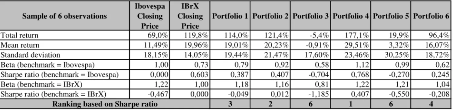
Sample of 6 observations
Ibovespa Closing
Price
IBrX Closing
Price
Portfolio 1 Portfolio 2 Portfolio 3 Portfolio 4 Portfolio 5 Portfolio 6
Total return 69,0% 119,8% 114,0% 121,4% -5,4% 177,1% 19,9% 96,4%
Mean return 11,49% 19,96% 19,01% 20,23% -0,91% 29,51% 3,32% 16,07%
Standard deviation 18,15% 14,05% 19,44% 21,47% 17,60% 23,46% 30,25% 18,72%
Beta (benchmark = Ibovespa) 1,00 0,73 0,79 0,92 0,58 1,12 0,99 0,62
Sharpe ratio (benchmark = Ibovespa) 0,000 0,603 0,387 0,407 -0,704 0,768 -0,270 0,245
Beta (benchmark = IBrX) 1,22 1,00 1,18 1,16 0,81 1,22 1,21 1,04
Sharpe ratio (benchmark = IBrX) -0,467 0,000 -0,049 0,012 -1,185 0,407 -0,550 -0,208
3 2 6 1 6 4
Ranking based on Sharpe ratio
Table 6. Results from rebalancing the portfolios annually.
Rebalancing Weekly Monthly Quarterly
Semi-annual Annual General
Portfolio 1 2 3 2 2 3 2
Portfolio 2 6 6 6 4 2 4
Portfolio 3 5 2 6 6 6 5
Portfolio 4 1 1 1 1 1 1
Portfolio 5 4 4 6 6 6 6
Portfolio 6 3 5 3 3 4 3
Table 7. General ranking of all strategies.
The bootstrap of the weekly returns, shown on Table 8 confirmed the superiority of the strategy of
Portfolio 4 over the others as seen on Table 7. The T- and F-Tests on Table 8 show that Portfolio 4 has
a bigger variance and mean return than both market indexes IBrX and Ibovespa, which is reflected on
its high Sharpe ratio, and with 5% of significance the returns from Portfolio 4 are superior to the
returns from both market indexes. This can be seen when we look at the lower and upper bounds of
confidence intervals. So considering the whole sample of 294 weeks, thanks to the bootstrap we can
say that the strategy held by Portfolio 4 was the best one.
Returns from bootstrapping
Ibovespa Closing Price IBrX Closing Price
Portfolio 1 Portfolio 2 Portfolio 3 Portfolio 4 Portfolio 5 Portfolio 6
Mean 73,3% 125,6% 145,2% 77,4% 98,3% 249,5% 127,6% 131,6%
Standard deviation 77,8% 66,2% 68,6% 77,5% 93,8% 103,1% 79,6% 70,7%
Confidence Interval - lower bound -78,0% 1,3% 10,1% -75,7% -78,3% 53,1% -30,1% -6,5%
Confidence Interval - upper bound 233,0% 260,0% 287,2% 231,5% 288,0% 453,8% 289,2% 275,2%
Variation coefficient 1,062 0,527 0,472 1,001 0,954 0,413 0,624 0,537 Mean / (Confidence interval upper minus lower bound) 0,236 0,485 0,524 0,252 0,268 0,623 0,400 0,467 F Test for difference of variances Portfolios x Ibovespa 1,382 1,286 1,009 1,452 1,756 1,046 1,213
F Test for difference of variances Portfolios x IBrX 1,382 1,075 1,370 2,008 2,427 1,446 1,139
T Test for difference of means Portfolios x Ibovespa 0,000% 0,000% 0,395% 0,000% 0,000% 0,000% 0,000% T Test for difference of means Portfolios x IBrX 0,000% 0,000% 0,000% 0,000% 0,000% 8,229% 0,000%
Sharpe Ratio (benchmark = Ibovespa) 1,048 0,053 0,267 1,709 0,682 0,825
Sharpe Ratio (benchmark = IBrX) 0,287 -0,621 -0,291 1,202 0,026 0,086
2 6 5 1 4 3
Ranking based on Sharpe ratio
F-Test T-Test
(grey square) Different variances at the 5% significance level. (grey square) Equal mean returns at the 5% significance level.
Table 8. Results from the bootstrap of 294 weekly returns.
To test the robustness of the strategy of Portfolio 4, we performed 5000 simulations of 52 weeks
chosen randomly of investment on the stock market following the six strategies. Portfolio 4 showed
again a superior performance compared to its peers and the market indexes, as we can see on Table 9.
At the same time Portfolio 1 was again the second best strategy. So following the brokerage houses’
recommendations through a naïve strategy (Portfolio 1) or a simple but more elaborated one (Portfolio
4) the investor may beat the market indexes Ibovespa and IBrX consistently. These results are
confirmed through the T- and F-tests performed on the empirical distributions obtained from the Monte
Carlo simulation at the 5% significance level.
Returns from simulation
Ibovespa Closing Price IBrX Closing Price
Portfolio 1 Portfolio 2 Portfolio 3 Portfolio 4 Portfolio 5 Portfolio 6
Mean 12,7% 22,2% 25,5% 13,5% 17,0% 44,2% 22,9% 22,8%
Standard deviation 29,5% 25,2% 25,9% 28,7% 36,7% 39,0% 30,6% 27,0%
Confidence Interval - lower bound -44,3% -25,1% -25,4% -41,5% -53,0% -29,7% -34,0% -27,7%
Confidence Interval - upper bound 73,4% 72,3% 76,9% 70,4% 90,9% 121,8% 84,3% 78,3%
Variation coefficient 0,431 0,880 0,983 0,471 0,463 1,136 0,751 0,845 Mean / (Confidence interval upper minus lower bound) 0,108 0,227 0,249 0,121 0,118 0,292 0,194 0,215 F Test for difference of variances Portfolios x Ibovespa 1,378 1,299 1,062 1,547 1,739 1,070 1,197
F Test for difference of variances Portfolios x IBrX 1,378 1,061 1,297 2,133 2,397 1,474 1,152
T Test for difference of means Portfolios x Ibovespa 0,000% 0,000% 9,021% 0,000% 0,000% 0,000% 0,000% T Test for difference of means Portfolios x IBrX 0,000% 0,000% 0,000% 0,000% 0,000% 7,689% 9,759%
Sharpe Ratio (benchmark = Ibovespa) 0,492 0,027 0,117 0,809 0,335 0,374
Sharpe Ratio (benchmark = IBrX) 0,128 -0,302 -0,140 0,567 0,026 0,025
2 6 5 1 4 3
Ranking based on Sharpe ratio
F-Test T-Test
(grey square) Different variances at the 5% significance level. (grey square) Equal mean returns at the 5% significance level.
Conclusions
As shown previously it is possible to beat the Brazilian market indexes Ibovespa and IBrX following
the analysts’ stock recommendations. The best strategies are buying only the recommended stocks
(Portfolio 1), buying the recommended stocks whose target and market prices difference is bigger than
25% and lesser or equal than 50% (Portfolio 4). These two strategies beat the market and the other
strategies tested not only on absolute return but also on a risk-adjusted basis through the analysis of the
Sharpe ratio. To confirm these results we performed a bootstrap analysis of the 294 weekly returns
from the sample, and a simulation of a year (52 weeks) of random investment on the stock market
following the six strategies.
Those are interesting results that shows that analyst’s recommendations add value in Brazilian Market,
and also that the Efficient Market Hypothesis does not hold in our market, as it is possible to earn
significant returns with public information. Transaction costs were not considered but we believe that
they do not have a significant impact over our results.
As further research we suggest several issues related to the data base. There are several questions to
answer. The following are some of them:
a. Is there a best investment company to follow?
b. The forecast target prices are useful?
c. With are the main characteristics of the recommended companies?
References
1. Bacman, J. F. and Bolliger, G. (2001) - Who Are the Best? Local versus Foreign Analysts on the Latin American Stock Markets – Working Paper - University of Neuchâtel – Neuchâtel - Switzerland
2. Bae, K. H.; Stulz, R. M.; Tan, H. (2005) – Do Local Analysts Know More? A Cross Country Study of the Performance of Local Analysts and Foreign Analysts Working Paper –NBER w11697 - September
3. Barber, B. ; Lehavy, R. ; McNichols, M. & Trueman, B. (2003) – Prophets and Losses:
Reassessing the Returns to Analysts’ Stock Recommendations – Financial Analysts Journal - 59 -2: 88-96 - March/April
4. Barber, B.; Lehavy, R.; McNichols, M. (2001) Can investors profit from prophets? Consensus Analysts Recommendations and Stock Return– The Journal of Finance - 56 - 2:531-563 - April 5. Black, F. (1973) – Yes Virginia, There is Hope: Tests of the Value Line Ranking System –
Financial Analysts Journal – 29: 10-14, September/October
6. Bonini, S. ; Zanetti, L. ; Bianchini, R. (2005) – The Predictive Power of Analyst’s Target Prices – Annals EFMA 2005 Annual Meeting
7. Copeland, T. & Mayers, D. (1982) – The Value Line Enigma: A Case Study of Performance Evaluations Issues – Journal of Financial Economics, 10: 289-321 - November
8. Crichfield, T. ; Dyckman, T. & Lakonishov, J. (1978) – An Evaluation of Security Analysts’ Forecast – The Accounting Review –53 - 3: 651-668 – July
9. Efron, B. (1979) – Bootstrap methods: Another look at the Jacknife. – Annals of Statistics – 7 – 1-26
10.Jegadeesh, N.; Kim, J.; Krishe, S. D.; Lee, C. M. C. (2002) – Analyzing the Analysts: When do Recommendations add Value? – The Journal of Finance – 54 – 3:1083-1124 - June
11.Juergens, J. L (1999) – How do Stock Markets Process Analysts’ Recommendations? Working Paper – Arizona State University
12.Metrick, A. (1997) – The Equity Performance of Investment Newsletters – Discussion Paper 1805 – Harvard Institute of Economic Research – Harvard University – November
13.Mikhail, M. B.; Walter, B. R.; Willis, R. H. (2004) – Do Security Analysts Exhibit Persistent Differences in Stock Picking Ability? – Journal of Financial Economics 74 - 1: 67-91 - October 14.Shelton, J.P. – The Value Line Contest: A Test of the Predictability of Stock Prices Changes –
Journal of Business – 1967, 40 – 3: 254-269 - July
15.Szakmary, A.; Lancaster, K. (2005) – An Examination of Value Line Long Term Projections – Working Paper - University of Richmond
16.Womack, K. L. (1996) – Do Brokerage Analyst’s Recommendations Have Investment Value? – The Journal of Finance –51 – 1: 137-167 - March