r __
•
•
•
•
•
セN@
,
SEMINARIOS DE ALMOÇO
•
•
FUNDAÇÃODA EPGE
•
GETUUO VARGAS•
•
•
•
Deunionization in the US: A panel data
•
•
analysis trom 1973 to 1999
•
•
•
•
•
•
•
•
FERNANDO DE HOLANDA BARBOSA
FILHO
•
•
•
•
(New York University)
•
•
•
•
•
•
Data: 29/07/2005 (Sexta-feira)
•
•
Horário: 12 h 15 min
•
•
•
•
セD@
Local:
•
Praia de Botafogo, 190 - 11
0andar
•
FGV
Auditório nO 1
•
EPGE
Coordenação:
•
Prof. Luis Henrique B. Braido
•
e-mail: [email protected]
•
•
•
•
•
•
,
-
••
•
•
.'
•
•
•
•
•
•
•
•
•
•
•
•
•
•
•
•
•
•
•
•
•
•
•
•
•
•
•
•
•
•
•
•
•
•
•
•
•
•
•
•
•
•
•
•
•
Deunionization in the US: A Panel Data Analysis
from1973 to 1999.
Fernando de Holanda Barbosa Filho
July 27, 2005
Abstract
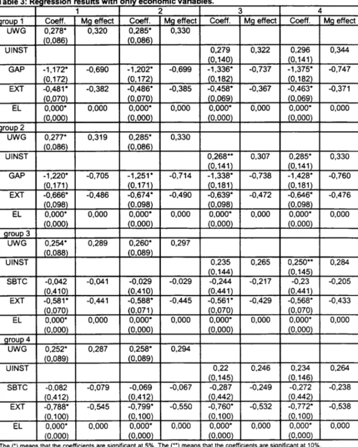
There are four different hypotheses analyzed in the literature that ex-plain deunionization, namely: the decrease in the demand for union rep-resentation by the workers; the impaet of globalization over unionization rates; teehnieal ehange and ehanges in the legal and politieal systems against unions. This paper aims to test alI ofthem. We estimate a logis-tie regression using panel data proeedure with 35 industries from 1973 to 1999 and eonclude that the four hypotheses ean not be rejeeted by the data. We also use a varianee analysis deeomposition to study the impaet of these variables over the drop in unionization rates. In the model with no demographic variables the results show that these economic(tested) variables can account from 10% to 12% of the drop in unionization . However, when we include demographic variables these tested variables can account from 10% to 35% in the total variation of unionization rates. In this case the four hypotheses tested can explain up to 50% ofthe total drop in unionization rates explained by the modeJ.
1 Introduction
In the late 70's, the rate ofunionized workers was 30% in the U.S. while in 2000 it was only 14% (Farber and Western, 2000). Regarding the UK, this rate was above 55% and then it dropped to below 30% in the same period (Machin, 2000, 2002). There are several empirical as well as theoretical studies that have anempted to test the causes of this decline.
The literature has been using different hypotheses to explain this reduction ofunion-ization. One hypothesis relates this deunionization to changes in the legal and political system. These changes would create an economic environment more hostile to union 's activities. Key facts related to this are the 1981 air-traffic controller strike, the Rea-gan's National Labor Relations Board(NLRB) appointments in 1983 for the US, and the Thatcher govemment in the UK.
their conclusion they claim that changes in the economic environment that made union represer:.tation of less value or more costly to employees may be the cause of deunion-ization. They belíeve the drop in union election activities is a marginal contributor to deunionization.
In
Farber and Western (2000) the increase in global competitiveness and capital mobilíty are mentioned to be other possible hypotheses for deunionization. However, Farber and Krueger(1992) point out the drop in the workers demand for union repre-sentation as a key factor explaining the union membership decline in the USoAnolher possible explanation for deunionization relates technological advance and the decision of union members to leave the union due to the action of market forces, which iIl:crease the tensions among workers inside the unions and beyond its breaking point.
Acemoglu, Aghion and Violante (2001) pointed out this technological hypothe-siso They analyze unions as rent-seeking agents imposing a contract on the firm or as efficiency-enhancing unions, where the union induces training to the workers, or provides insurance to themselves. Their study makes use of the skill biased techni-cal change as the driving force that generates deunionization because it increases the outside option of skilled workers.
This paper intends to contribute to the existing literature for the following reasons. First, it builds a pane I data with 35 industries from 1973 to 1999 containing data on US union rates and other variables that may explain deunionization. Second, it tests at the same time the four different hypotheses presented in the literature to explain deunion-ization. They are: the decrease in the demand for union representation by the workers; the impact of globalization over unionization rates; technical change and changes in the legal and polítical systems against unions. Third it evaluates the impact of these hypotheses on the decline of unionization rates through a variance analysis decompo-sition.
This paper uses a pane I data to identify empirically which of the above factors are relevant and also to measure their contribution in the drop ofunionized workers in the US. We test the four hypotheses mentioned above using a panel data estimation based on 10gisLC regressions in which we encompass these four hypotheses. We estimate two different models: one with only the variables that represent the hypotheses being tested and other with the addition of demographic variables. Both estimations give us similar results. We conclude that the four hypotheses we have tested, namely: the decrease in the demand for union representation by the workers; the impact of globalization over unionization rates; technical change and changes in the legal and political systems against unions can not be rejected by the data.
We also use a variance analysis decomposition to study the impact ofthese variables over the drop in unionization rates. Once more, we analyze two different models: one that does not include demographic variables and other that does include it. In the model without demographic variables, we find that the economic(tested) variables can account for 10% to 12% in the decline ofunionization while industry specific effects (random
andlor fu:ed) account for around 80% ofthe total variation.
In
the model that includes demographic variables, the tested and demographic vari-ables explains up to 63.3% ofthe total variation in the unionization rates while industry2
セ|@
•
•
•
'.
•
•
•
•
•
•
•
•
•
•
•
•
•
•
•
•
•
•
•
•
•
•
•
•
•
•
•
•
•
•
•
•
•
•
•
.,
•
•
.'
•
•
•
•
•
•
•
•
•
•
•
•
•
•
•
•
•
•
•
•
•
•
•
•
•
•
•
•
•
•
•
•
•
•
•
•
•
•
•
•
•
•
•
•
•
specific (random and/or fixed) effects can account for around 35%. The tested variables accounts from 10% to 35%. In this case the four hypotheses tested can explain up to 50% of the total drop in unionization rates explained by the mode!.
This paper is organized as follows: the next section presents a review of the litera-ture, section 3 describes the data sources, the methodology used and describes the data series. Section 4 presents the model and the methodology used to estimate it. In section 5, reports our empirical finds and discuss them. Section 6 contains a variance analysis decomposition that measures the impact of each factor in the unionization rates decline; and section 7 sums up with the concluding remarks.
2 Review of the Literature
The impact of unions on the wage structure is one of the most explored subjects on unions studies. Works in this area range from studies concemed about the effect of the unions on wages and the existence of wage premium to the union impact on wage distribution.
The first studies about the union effect on wages argue that unions would increase wage inequality in the U.S. On the one hand Friedman( 1956) argues that craft unions would be more efficient in raising wages than industrial unions. Therefore, the wage of more skilled workers would be even higher. Rees(l962) follows the same ide a based on the fact that union membership at the 50's was concentrated among the top of the earnings distribution. On the other hand, Reynolds and Taft(l956) analyze the wage structure in different industries and conclude that unions have not increased wage in-equality. They claim that it was even possible that unions decreased wage inin-equality.
Lewis(1963) studies the correlation between union wage differential and wage lev-eis. He says that unionism increased inequality across industries by two to three per cento On the contrary, Stafford( 1968), Rosen(l970) and Johnson and Youmans(l971) concluded that unions compress wages because it raises the low skilled wages relatively more than the high skilled wages.
In a very infiuential survey where he examined approximately 200 studies on the effects of unions on wages, Lewis( 1986) concludes that methodological1y the best way to estimate the size effect ofunions on wages is to run OLS equations with wages on the left side, as dependent variables, and union status and other control variables on the right side, as independem variables. He also concluded that the impact of unions on wages in the US economy creates a wage differential around 15% and it is very stable in the period between 1967 and 1979.
Subsequent works confirm the conclusion ofLewis( 1986). Hirsch and Schumacher(2002), Hirsch and Macpherson(2002) and Hirsch et al(2002) analyze wage gap over time and along with the confirmation of its stability over time, conclude that it has experienced a decline in recent years. Bratsberg and Ragan(2002) analyze the private sector wage gap between 1971 and 1999. They reassure the stability of the union wage premium over time and also notice the decline in recent years.
Card( 1996) uses Currem Population Survey(CPS) data from 1987 and 1988 to study the effects ofunions on the wage structure. He uses a technique that accounts for
classification errors, potential correlations between union status and unobserved pro-ductivitf, His analysis separate different skilI groups and results suggest that unions raise wa.ges more for unskilIed groups than for skilled groups. He observes two differ-ent pattems of bias selection between high and low skilIed groups. He discovers that there is a positive selection among low skilIed workers(of unobserved ability) and a negative selection among high skilIed workers.
Raphael(2000) uses the CPS displaced workers supplement files from 1994 to 1996 to study the effects of union membership on weekly eamings. His conclusion sup-ports Card(1996). He finds a positive selection for low skilled workers and a negative selection for high skilIed workers.
The union membership rates are dropping steadily since the 70's in the USo There are many studies connecting this fact to another welI known in the US economy: the increase in wage inequality. Others try to find and explain the causes ofthis decline on union representation in the USo
Card(200 1) uses the CPS micro data for 1973, 1974 and 1993 to study the effect of union membership changing on trends in male and female inequality, for the public and private sector. He realizes unions act in the same way in the private and public sector and unionization rates felI for men and women. He also finds that even afier controIling for unobserved skills there is a wage premiurn for union workers. Finally, he concludes that the decrease in unionized workers can account for 15-20% ofthe increase in male wage inequality.
Di Nardo, Fortin and Lemieux( 1996) use CPS data from 1979 to 1988 and point out that shifts in unionization can explain 15-20% of the increase in wage inequality for men, and 3 % for women.
Freeman(l993) uses the CPS longitudinal matched for men from 1978 to 1988
and says that 20% of the increase in the male log eamings in the period is due to deunionization.
Farber( 1990) uses May CPS data from 1973 to 1984 to show that the rate ofunion-ized workers drops sharply. He points out two possible reasons for this decline. The first is a11 increase in employer resistance due to increase in market competition; the second is a decrease in the demand for union representation by the workers.
Farber and Krueger( 1992) use the May CPS data for 1977 and the merged outgoing rotationsroup data from the CPS(morg-CPS) for 1984 and 1991 in order to analyze the decline in union membership rate in the US and the difference in unionization rates between the US and Canada. They conclude the decline in the US is due to a drop in the worker's demand for umons. What's more, that very little ofthis drop can be explained by shifts in the composition ofthe labor force. FinaIIy, the differences between US and Canada are due to demand and supply differences.
Farber and Weslern(2000) examine monthly data on NLRB union representation elections to determine if changes in the adrninistration of the NLRA cause a reduction in the leveI of union organizing activity. They also tried to reconcile the drop in the union organization activity with key political events, like the PATCO strike of 1981 and the Reag,m majority in the NLRB in 1983. They show the drop in union organizing activity happened before these political events. They also point out the drop in union organizing activity accounts only for a smaIl fraction ofthe drop in unionization rates.
4
,.
•
•
'.
•
•
•
•
•
•
•
•
•
•
•
•
•
•
•
•
•
•
•
•
•
•
•
•
•
•
•
•
•
•
•
•
•
•
•
•
•
•
•
•
•
•
•
•
.,
•
•
.'
•
•
•
•
•
•
•
•
•
•
•
•
•
•
•
•
•
•
•
•
•
•
•
•
•
•
•
•
•
•
•
•
•
•
•
•
•
•
•
•
•
•
•
•
•
They indicate changes in economic environrnent that made union representation ofless value to worker or more costly to employers; and the increase in global competitiveness and capital mobility as important factors explaining the drop in unionization rates.
Farber and Western(200 1) make an empirical time series analysis ofNLRB monthly organizing elections. They conclude that sharp decline in the number of organizing elections preceded the PATCO strike of 1981 and the Reagan majority in the NLRB in
1983.
Acemoglu, Aghion and Violante (2001) analyze unions as rent-seeking agents im-posing a contract on the firm or as efficiency-enhancing unions, where it induces train-ing to the workers, or it provides insurance to themselves. They use skill biased tech-nical change as the driving force that generates deunionization. This also generates an increase in wage inequality.
The above studies may bring us a conclusion that unions compress wages differen-tials in the U.S. It happens because the union effect on wages is higher for low skilled workers(in the bonom of income distribution) than for high skilled workers. We can also say that there is a union membership premium. Therefore, we may think that union membership is a good to be purchased, and this wage gap is the good offered by a union.1
3 The Data
We use different data sources to construct the series used in this paper. For the union-ization rate, wage premium and the demographic variables, the CPS is used. For the openness index, we use the Center of International Data(CID) at UCD directed by Robert Feenstra, OECD and Bureau ofEconomic Analysis(BEA) data. The series that measure technological progress are from the BEA and Cummins and Violante(2002). These series cover the period between 1973-2002 and are at an industry leve!.
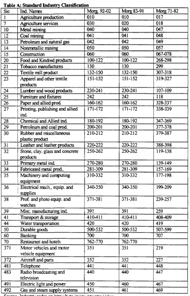
Unfortunately, not alI the industries or sectors appear in the different data sources that we have. Consequently, the analysis is carried on only with the 35 industries that show up in all the different sources and allow to have a balanced pane!. The 35 different industries in our data follow a Standard Industry Classification(SICi.
3.1
Unionization Rate
The CPS is the most important source of information to construct union membership series. Questions about union membership were regularly included in this survey in 1973. This data is reported in the mayCPS between 1973 and 1981. The CPS pro-vides data on a very comprehensive set of variables. The union membership series constructed here is based on wage and salary workers 16 years old and over, in or-der to make it compatible with the sample from 1983 to date. In the year of 1982 there is no data on union membership available3 . In 1983 the data on union member-ship starts being released in the outgoing rotation groups ofthe CPS(CPSmorg). The
1 Unions can provi de difTerent services to its members and the wage gap is one ofthem. In our analysis we use it because it has more accurate available data.
2 The sic classification is presented in the appendix. 3 Therefore we interpolate the years of 1981 and 1983.
CPSmorg reports results on wage and salary workers that ages 16 and over. The data is collected in the following way: an individual is interviewed during 4 months consec-utively and then ignored for 8 months. If the individuaIs move, they are not followed, rather the new occupants are interviewed. Since 1979 the individuais in months 4 and 8 were asked questions about earnings, union membership and so on. The mayCPS data was downloaded from the NBER web site from 1973-1981. The CPSmorg data was obtained in a CD-ROM acquired from the NBER and contains the years between 1979-2003.
In order to obtain the correct statistics to the US economy, both samples contain weights that are used to compute the unionization rate and also the wage gap4.
The unionization rate and the wage gap were computed in an industry specific way. The unionization rate was computed using the following formula:
JoJ
L
(fVEj )sijdijUNi
=
ェ]セ@
(1)L
(WEj)Sijj=1
In this expression WEj is the weight associated with each observation j, Sij and
d.;j are dummy variables. These take value one if the observation is from sector i for Sij and )fthe worker is a union member for dij and zero otherwise.
3.2
Wage Premium
The wage premiurn is the "premiurn" received by union members as a higher wage, because as unions are well known as rent extractors, they are able to obtain higher wages from firms. Therefore, we expect a high wage premiurn to have a positive impact in the ra:e ofunionized workers.
The wage premium is measured as the ratio between union and nonunion wages. We call union wage by Wu and the nonunion wage by w. We computed the wage
prernium in two different ways.
The j5rst is a naive one: we measure the average wages received by unionized and non-unionized workers and take the ratios. In order to compute it, we proceed in the following way:
Wi= M
(2)
L
(EWj)sij(l - dij )j=1 M
L
ej(EWj)sijdijWui = M
j=1
(3)
L
(EWj)Sijd.;jj=1
---
4 There are specific weights associated with each interview. One weighl for lhe populalion value and olher for lhe earnings.6
•
••
•
•
'.
•
•
•
•
•
•
•
•
•
•
•
•
•
•
•
•
•
•
•
•
•
•
•
•
•
•
•
•
•
•
•
•
•
•
•
•
•
•
•
•
•
•
•
•
..
.
,•
•
.'
•
•
•
•
•
•
•
•
•
•
•
•
•
•
•
•
•
•
•
•
•
•
•
•
•
•
•
•
•
•
•
•
•
•
•
•
•
•
•
•
•
•
•
•
•
In equations 2 and 3 e j represents the eamings received, EvVj represents the
earn-ings weights, Sij represents the sector and dij is the union dwnmy variable. The wage premium is given by the ratio:
W.G N = -Wu
W
(4)
Equation 4 represent the wage gap obtained by the naive measure(the subscript N indicates naive). This naive measure does not necessarily represent the wage premium received by a union member because it does not control for individual characteristics that can influence wages and union selection. Then, a measure that take this character-istics into account is necessary.
In order to have a wage premium associated only with the fact that the worker is a union member, we need to control for the observed abilities. Therefore, we separate the sample in gender, education levei, age and race. High skilled workers are those with a high school degree. The sample was divided into workers 01 der and younger that 35; white and nonwhite. We have created 16 different groups then.
Ali the workers in an industry were classified into one of this 16 groups. Each group have its dummy variable
G
gi , being i the industry and g = 1, ... , 16 represents the group.M
L ej(EWj )Ggi(l - セェI@
j=1
Wgi = M (5)
L(EWj )Ggi(l- dij )
j=1
M
L ・ェHewェIgセェ@
j=1
Wugi = M (6)
L (EWj)Gdij j=1
In equations 5 and 6 ej represents the eamings received, EWj represents the
eam-ings weights, G g1 represents the classification group and セェ@ is the union dwnmy vari-able.
We use the union and the nonunion wage received by each group in each industry to calculate the wage gap within each group:
WGgi = Wugi (7)
Wgi
Afier obtaining the wage gap within each classification group, we need each group weight to obtain the wage gap in that industry. The classification group weights are obtained in the following way:
M
L (W Ej )SijGgi j=1
DG
9 = -1...:,6--:M-:---(8)
L L (WEj)SijGgi g=1j=1
16
Obviously we have
L
DGg=
1. Then, we obtain the industry specific wage gap:g=l
16
WGi
=
L
(DGg)(WGgi ) (9)g=l
3.3
Openness Variable
The data are from the Center ofInternational Data(CID) , the OECD and the Bureau of Economic Analysis(BEA) websites. The input-output matrix obtained from the OECD cover the period from 1972 to 2002. Unfortunately, this series do not cover ali years. The input-output matrix covers the years of 1972, 1977, 1982, 1987, 1992, 1997-2002. The missing observations are filled with interpolation arnong the existing ones. The OECD and the BEA data are used to obtain the total GDP per industry.
The Feenstra data is used to obtain the total imports and exports per industry. We use two different measures of openness: the import penetration and externaI trade industry share.
The import penetration index is measured in the following way:
IP = J\!!i (10)
, GDPi
As it can be seen it measures the share of imported goods in each industry. The externaI trade industry share is measured by:
ETI8-= (Xi
+
Mi )• GDPi
(11 )
The ETIS measures the transactions with the rest of the world that an industry has as a share of its GDP.
3.4
Institutional Index
This variable tries to measure the impact of anti-union legislation that supposedly hap-pened in the US, in the beginning ofthe 80's.
Since there is no variable that measures directly the institutional change against unions, we use the number of recognizing elections hold each year as a proxy of this movement against unions. As this is a wide eeonomy effeet, this index is not industry specific. This data is obtained frorn NLRB.
3.5
Technological Measures
The idea behind the effeet of teehnology on unions oeeurs in two different ways. The first one is caused because an inerease in technology creates an incentive arnong skilled workers to leave a union because the new teehnology benefits this group vis-à-vis the other. The seeond aspeet relates the technologieal gap. We expect industries that are far away from the teehnologieal frontier to be less eompetitive. As these firrns are less eompetitive, unions ean not extraet high rents and therefore it affeets unions negatively. The variables that measure teehnologieal advanee are obtained from the BEA web-site and :Tom Cummins and Violante(2002).
8
-••
•
•
••
•
•
•
•
•
•
•
•
•
•
•
•
•
•
•
•
•
•
•
•
•
•
•
•
•
•
•
•
•
•
•
•
•
•
•
•
•
•
•
•
•
•
••
•
•
.'
•
•
•
•
•
•
•
•
•
•
•
•
•
•
•
•
•
•
•
•
•
•
•
•
•
•
•
•
•
•
•
•
•
•
•
•
•
•
•
•
•
•
•
•
•
We obtain the multifactor productivity, the labor productivity and the capital pro-ductivity from the BEA website.
The other two technological measures used are the technological gap and a measure of non neutral technological advance, that we call skill biased technical change(SBTC).
3.6
Demographic Variables
All the six demographic variables used are obtained from the mayCPS from 1973 to 1999 and from the morgCPS from 1983 to 1999. The demographic variables chosen are ratio of white, male, married and full time workers and years of education and experience per industry, once more using the Standard Industry Classification(SIC).
3.7
Data Description
The variables used in the estimation procedure are measured in ao industry specific basis. As mentioned before, we use 35 industries selected using the Standard In-dustry Classification(SIC). The variables we will use are the following: unionization rate(ú' Nit ), wage prernium(W Git ), technology( Ait ), import penetration (
clt'!>;.
) ,
ex-ternai trade sectorial share (
X/;'i!;J;;.i
t) and number of union recognition elections( Elt ).
Despite this variables we also make use of several demographic variables like: educa-tion, marital status, experience, race, sex and full time ratios. The education variable measures the average years of education per industry. Experience is measure in aver-age years and follow a standard measure in the literature: experience equals aver-age minus years of education minus five. We also use the ratio of white employees per industry, the ratio ofrnarried employees and full time workers in each industry.
Before presenting the model, we describe the data.
3.7.1 Unionization Rate
As expected, the unionization rate presents a decline in all but one of the sectors under study between 1973 and 1999. I t can also be observed that this decline has a stable and long pattern, as seen below.
Graph 1: Unionization Rate
0.2000
0.1000
0.0000
C")
...
'"
<D ... co'"
o=
N C")...
'"
<D ... co'"
o c;; N C")...
'"
<D ... co... ... ... ... ... ... ... co co co CD CD CD CD co CD
'"
'"
'"
'" '"
'"
'"
'"
セ@ セ@
'"
セ@ セ@ セ@'"
セ@'"
セ@ セ@ セ@ セ@ セ@ セ@'"
セ@'"
セ@ セ@ セ@ セ@ セ@'"
セ@ セ@セ@'"
セ@'"
セ@'"
セ@The graph helps to observe that there are two distinct groups in this data sample. The fus': one that lost a huge part of its members but remained with relatively high unionization rates. The second one that kept it low unionization rate, even losing part of its members.
1t is .nteresting to observe that despite the union losses over the período the fifteen sectors that had a higher unionization rate in 1973 remain the same in 1999 but for one sector, as can be seen in the following table.
lO
•
••
•
•
••
•
•
•
l-un1
: --_ .. un7
•
I un12un13
•
-un14
•
-un20
•
--·-un21
-un22
•
un23
un24
•
un25
•
un26
un27
•
un28
•
un29
un30
•
-un31
un32
•
un33
•
un34
un35
•
'"
'"
セ@•
•
•
•
•
•
•
•
•
•
•
•
•
•
•
•
•
•
•
•
•
•
•
•
•
•
•
•
•
••
•
•
••
•
•
•
•
•
•
•
•
•
•
•
•
•
•
•
•
•
•
•
•
•
•
•
•
•
•
•
•
•
•
•
•
•
•
•
•
•
•
•
•
•
•
•
•
•
T abIe 1: Uricn rales t v IrxtsITv per
Yea-1973 1981 1990 1999
1coa1rriring 74.68"tC
macr
vehicIe 65.77o/cmacr
vetidedes 48.19"1< motcrvehde2 motcr veticIe 70.99"1< tobac:co 57.82"1< telE!ltlone 45.72"1< Bel iセ@ ald Pov.er
3 Prirrav metal. 61.63% waerlra1sp 55.99"1< Prirrsy metal. 4121°1< Prinay metal.
4 59.v.:: 54.67o/c coai rriring 37.86"1< v.atertralsp
5 v.ater tralsp 56.53'* pイゥセュ・エ。iN@ 53.96'* loaoer ald alLpod 37.38'* coai rririlR
61paper ald alLcrod 56.41o/c coai rrinirQ 5O.25o/c 8et Iktt ald Pov.er 36.56"1< aircraft a1d pa1
7 stcrecJav 5O.7Oo/c 8et. liçH and Pov.er 43.59"1< aircraft ald pa1 31.86"1<
8 ni:lber a1d rrisc 46.40"1< I papel" a1d alLprod 43.51o/c Igas&steaT1 30.83'* papel" a1d all.prod 9 focxl 42.93o/c food 42.35o/c water lra1sp 30.44°1< tobac:co
10 Fab. lVet A'ociJct 42.79o/c Pet. ald CoaI crod. 40.73'* stonecJav 27.96"1< QaS&stean 11 Bel Iiçtlt ald Pov.er 42.42o/c 19as & stE9l1 36.7Oo/c Pel. ald CoaI prod. 26.88% Pel. a1d CoaI crod.
12 Pet. an::I CoaI prad. セRNRRッO」@ stoneday 35.57o/c food 25.91°1< focxl
13 TransQ. ald SIoraQe 4O.28o/c Fab. lVet A'ociJct 34.74o/c Fab. lVet ProcLd 23.82"/c, stonedav
14 airaál a1d pa1 39.53'* aircraft ald pa1 28.48o/c Ncm1et. MrirQ 23.66"1< Trcnsp. a1d StaaQEl
151gas & stE9l1 36.31'* Normet. Mring 28.42"1< Tra1SP. ald Storage 23.35o/c ni:lber a1d rrisc
161apparei and cXher text 34.87o/c cherricaI 28.16'* tobac:co 18.32"1< Fab. lVet ProdI.d
17 セN@ & COITll. 33.7Oo/c Sec. macho ald SW. 27'(lIO/C nttler ald rrisc 16.23"1< leaIher a1d crod 18 8ec. macho ald sw· 33.51o/c lappa-eI ald cXher text 26.54o/c chernicaI 15.42"1< radoa1dtv
19 tOOacco 32.84o/c Mach. & COITll. 26.29"1< laDPErei and dher text 15.09"1< Ncm1et. Mring 20 lLrTtler v.ood 30.12'* Trcnsp. and StaaQe 26.15% 8ec. macho ald SW. 15.<ll,* 8ec. mach. an::I SW.
21 Msc. Man. ind. 29.95o/c l.J..ntler v.ood 25.90"1< Mach. & COITll. 14.39"1< Mach. & COITll.
22 cherrical 28.27o/c nbber ald rrisc 24.94'* l.J..ntler v.ood 12.82"1< chernicaI
123 t-bmet. MnirQ 27.20"1< Funittre and fix. 2427o/c radoaldtv 12.30"1< rest a1d t"d 24 leaIher ald prod 26.41% iセNーィ@ 17.22% Funittre ald fix. 12.27"1< l.J..ntler v.ood
25 Fl6nitLre ald fix. 24.84o/c leaIher a1d crod 16.73'* leaIher ald prod QQNTRBセ@ appa-eI a1d cXher text
26 1 Drint, p.b ald ali 24.27% I Drint, p.b and ali 15.68'* IDriri. p.b ald ali 11.05o/c 1 Drint, pub ald ali 27 Ipro(. ph 20.96% Msc. Man. indo 12.23'* Msc. Man. indo 9.90"1< Msc. Mén. indo
28 racioa1dtv 17.83°1< durable 11.23% rest aldrot 9.49"1< Funittre a1d fix.
29 text rrill crod 13.52% radoandtv 9.84'* text rrill prod 9.12"1< Ipro(. ph
30 cUabIe 13.26% text rrill prod 7.86o/c lag·serc 8.21o/c text mil prod 311pet a1d nato QaS 7.48% 1 peI. ald na!. QaS 5.01% Ipret. ph 8.19"1< cUabIe
32lag.serc 5.61% lag.serc 3.63% I pet ald na!. QaS 5.07"1< lag.serc 33lag 3.53°1< lagr 3.<llo/c ónIbIe 4.04o/c I pet. a1d nato gas 34lba1kino 1.63% ba1kirQ 2.65o/c lag 1.9O"/c,
laa-35 rest. a1d t"dels 0.98% rest a1d t"d 0.69"1< Iba"IkirQ 1.40"1< ba1kirQ
The fabricated metallic products industry loses one position and the tobacco indus-try become one of the top 15 in unionization rates. It is important to notice that the tobacco industry already have a high unionization rate in 1973, 32.84%. It become one of the top 15 in 1999 with 24.81 % due to the fact that it suffer smaller losses than others that were ahead in 1973.
11
36.91o/c
35.59"1< 35.39"1< 30.92"1<
28.85o/c 28.45o/c
27.30"1< 26.30"1<
24.81o/c 23.83o/c
22.49"1< 22.42"1<
20.60%
19.96"1<
16.36o/c 15.71o/c
13.12"1<
12.23o/c 11.44o/c
10.92"1< 10.67"1< 10.33"1<
9.94o/c 8.74o/c
8.47"1<
8.25o/c
8.16"1<
6.94o/c
5.14°1< 5.09"1< 3.92"1<
3.11o/c
2.87"1< 2.46"1<
Table 2: Drop in unionization rates between 73 and 99 Absolute Relative
1 Coai Mining -45.83% apparel and other text -75.71% 2 Motor vehicle -34.09% Prof. ph. and EQ. -75.47% 3 Telephone -31.74% Misc. Man. Ind. -72.77% 4 Paper and AlI. Prod. -30.11% Fumiture and fixo -72.06% 5 Stone and clav -30.11 % LumberWood -70.99% 6 Rubber and misc. -30.04% Durables -70.45% 7 Fab. Met. Prod. -27.08% Mach. & Com-º, -68.33% 81Apparel and other te -26.40% Elec. Mach. and Sup_ -67.41% 9 Primary Metal. -26.24% Print. Pub and alI. -66.01% 10 キ。エ・イエイ。ョセ@ -25.61% rubber and misc -64.73% 11 Mach. & Comp. -23.03% Chemical -63.46% 12 Elec. Mach. and SUJl -22.59% fabmetal -63.29% 13 Misc. Man. Ind. -21.80% Text. mill prod. -62.34% 14 LumberWood -21.38% Pet. and n。エNセ。ウ@ -61.57%
15 food -20.50% Coai Mining -61.37% 16 Transp. and Storaae -20.31% stone clay -59.38% 17 Pet. and Coai prod. -19.73% Nonmet. Mining -57.92% 18 Chemical -17.94% t・ャセqィッョ・@ -53.76% 19 Fumiture and fixo -17.90% p。セ@ and AlI. Prod. -53.38%
20 Print. Pub and ali. -16.02% tイ。ョセN@ and Storage -50.43% 21 Prof. ph. and EQ. -15.82% Leather and Prod. -50.31% 22 Nonmet. Mining -15.76% Motor vehicle -48.02% 23 Leather and Prod. -13.29% food -47.76% 24 Gas & Steam -12.48% Pet. and Coai prod. -46.73% 25 Aircraft and Parts -11.08% water transp -45.30% 26 Durables -9.34% aer.serc -44.47% 27 Text. mill prod. -8.43% Bankine -44.35% 28 Tobacco -8.03% primetal -42.57% 29 Elet. lieht and Power -6.84% Gas & Steam -34.37% 30 radio and tv -5.60% radio and tv -31.40% 31 Pet. and Nat. gas -4.61% agr -30.28% 32 agr.serc -2.49% Aircraft and Parts -28.03% 33 agr -1.07% Tobacco -24.45% 34 Banking -0.72% Elet. light and Power -16.12% 35 Rest. and Hotels 8.96% Rest. and Hotels 916.34%
The industry that suffer the higher absolute losses of unionized workers are also the industries that have higher rates of unionized workers, as can be seen in the table above. However, ifyou compare the unionization rates to the 1973's unionization rates, the industries that had a higher percentage reduction in unionization rates are the ones that have a lower unionization rate. Therefore, despite the huge losses of unionized workers across the different industries observed, the high unionized ones protected themselves relatively bener than the low unionized industries.
The losses ofunion members range from 16.1% to 75.7% ofthe 1973 union mem-bers.
3.7.2 \\-age Premium
The two measures of wage premium used in this work present a similar pattem: a small decline in the wage prernium between 1973 and 1999. Both series can be divided into
two 、ゥヲヲ・Gセ・ョエ@ groups. One with the industries presenting a wage premium for union
12
セL@
••
•
•
••
•
•
•
•
•
•
•
•
•
•
•
•
•
•
•
•
•
•
•
•
•
•
•
•
•
•
•
•
•
•
•
•
•
•
•
•
•
•
•
•
•
•
•
.,
••
•
•
••
•
•
•
•
•
•
•
•
•
•
•
•
•
•
•
•
•
•
•
•
•
•
•
•
•
•
•
•
•
•
•
•
•
•
•
•
•
•
•
•
•
•
•
•
•
members and another including industries that do not have a wage premium.
In the naive measure, 17 industries did not pay a wage prernium in 1973 and this number increases to 19 in 1999. In the controlIed measure, the number of industries not paying a wage premium in 1973 is 14 and this number increases to 18 in 1999.
Another difference between the two measures is in the leveI. The adjusted measure is 10wer than the unadjusted for 24 of the 35 sectors studied. The majority of the sectors present a very stable declining path, but there are few sectors that present a great instability, specialIy from 1973 to 1981.
The adjusted wage prernium series have a lower variance across industries than the naive measure for 17 ofthe 27 years. And this variance is lower in 14 ofthe last 15 years.
We can say the adjusted series is less volatile than the unadjusted one and the two series showa slow decline in the wage prernium from 1973 to 1999.
3.7.3 Import Penetration and Externai Trade Industry Share
Both this series present the same pattern: a low leveI in the period between 1973 and the middle 80's, when a smalI increase can be observed in both measures and both had a huge increase in the late 90's.
The import penetration series
I Pit
presents an increase in alI but five sectors, whereas the externai trade industry share(ET I Sit) presents an increase in alI but three sectors. The last difference between these series is in their leveI, where we have the latter variable with a higher leveI.3.7.4 Technology
The technology variables used in the analysis are the technological gap, the SBTC, the multifactor, labor and capital productivity. The technological gap and SBTC have observations for all 35 industries while the multifactor, labor and capital productivity data have respectively 26, 27 and 24 industries available.
The technological gap shows a steady increase under the period of analysis. There are only two sectors that present a drop in the technological gap. In the others the increase in the technological gap range from 32.2% to 355% of the original 1973 tech-nological gap.
The SBTC shows a slightly increase under the period of analysis. There are eight sectors that present a drop. In the others the increase in SBTC range from 0.6% to 94.8% of the original 1973 SBTC.
The muItifactor productivity shows an increase from 1973 to 1999 in all but 4 in-dustries. This increase ranges from 0.1 % to 161.1 %. The labor productivity presents an increase for all 27 industries. This increase ranges from 5.8% to 541.8%. Differently the capital productivity present a decrease in 18 among the 24 industries available.
3.7.5 Union Recognition Elections
This is the only variable that is not industry specific in our analysis. This variable is an economy wide effect. In the graph below we can observe the number of elections
drop 62.5% in the period from 1973 to 1999 and a discontinuity in 1981. Before 1981, there is a steady decrease in the number ofunion recognition elections held. This same stable decrease in observed in the sample after 1981. In 1981 there is a discontinuity represented by the fierce drop in the number of elections held.
Graph 2: Union Recognilion Elleclions
9000 --.--.---.---,,--.---.---.----.---.• ---.---.
XセKQMMMMMMMMMMセMMMMMMセMMセセセMMMMMMセMMMMMMMMMMセセセMMMMMMM
WセK⦅MMMMセセMMMMセセ]M⦅イMMMMMMMMMMMMMMMMMMMMMMMMMMMMMMMMMMMM
VセK⦅MMMMMMMMMMMMMMMMMMMセ|ᄋᄋMMMMMMMMMMセMMMMMMMMMMMMMMMMセMMセMMMMセMMM
UセK⦅MMMMMMMMMMセMMMMMMMM|T⦅MMMMMMMMMMMMMMMMMMMMMMMMMMMMMMMMMMセMMMM⦅QMMセ@
\
セ@
TセゥMMMMMMMMMMMセMMMMMMMMセセセセセMMMMMMMMMMMMMMMMMMMMMMMMセMMMMM
---
...
セ@
セ@
SセセMMMMMMMMMMMMMMMMMMMMMMMMMMMMMMMMMMMMMMMセセセセMMセセセセセMMセセセ@
Rセ@
i
QセKセMMMMMMMMMMMMMMMMMMMMMMMMMMMMMMMMMMMMMMMMMMMMMMMMMMMMMMMMMMMMMMMMM
o j
'"
....'"
«> .... cc a> o ;;; N'"
....
'"
«>....
co a> o セ@ N'"
....'"
«>....
.... ....
....
.... .... ....
.... cc cc cc cc cc cc cc cc co a> a> a> a> a> a> a> cnセ@ セ@ セ@ セ@ セ@ セ@ a> セ@ セ@ セ@ セ@ a> セ@ セ@ セ@ a> セ@ セ@ セ@ a> セ@ セ@ セ@ セ@ cn
セ@ セ@ セ@ セ@
3.7.6 Demographic Variables
We use different demographic variables in order to understand their inftuence under the rate of unionized workers per industry. The demographic variables used here are measured in two different ways_ The first one is the ratio of individuaIs with this characteristics inside each industry. The variables that are measured in this way are: ratio ofmale, white , married and full time employees per industry. The second way is the measure of average years of education and experience in each industry.
The ratio of males variable is very stable between 1973 and 1999. We have that ali but five among the 35 industries had more than 50%of males among its employees in 1973. In 1999, ali but three have more than 50% of males. It is important to notice that, despite the increase in the number of industries with more than half of males in its labor force, there is a decrease in the ratio over the period for 24 of the 35 industries.
In ali the sectors the ratio ofwhite workers in each industry is above 60%. However it had a small decrease over the period for 25 ofthe 35 industries studied here. Despite this changes, the ratio ofwhite workers is pretty stable in the majority ofthe industries. The rate of married workers in each industry is very high but decreasing over the period of analysis. In 1973, ali the sectors had this ratio above 60%. In 1999, some industries have this ratio below 50%.
14
cc cn
a> cn
セ@ セ@
•
••
•
•
••
•
•
•
•
•
•
•
•
•
•
•
•
•
•
•
•
•
•
•
•
•
•
•
•
•
•
•
•
•
•
•
•
•
•
•
•
•
•
•
•
•
•
•
•
••
•
•
•
•
•
•
•
•
•
•
•
•
•
•
•
•
•
•
•
•
•
•
•
•
•
•
•
•
•
•
•
•
•
•
•
•
•
•
•
•
•
•
•
•
•
•
•
•
The rate of fulI time workers is very stable between 1973 and 1999. In 1973 all but the restaurants and hotels industries had the full time workers ratio above 60%, while restaurants and hotels had only 34% ofits employees as full time workers. In 1999, alI the industries have the ratio of full time workers above 70%.
The experience variable reports average years of experience per industry. This vari-able is slightly increasing. In 1973 all the industries had an average experience over 13 years, In 1999, this average increased to 17. Among the 35 industries 26 presented an increase in experience while 9 presented a decrease.
The education variable is a very stable one. We observe that 22 industries faced an increase in the average years of education while 13 observed a decrease. It is important to notice that every industry but agriculture has an average education over ten years.
3.8 Caveats
The use of several data sources made the data manipulation a very complex work. We use the different standard industry classification (SIC) tables available in order to correct the changes of this classification over the years. Three different SIC that also cover three periods: 1971-1982; 1983-1991 and 1992-2002 are used.
Putting together alI different data sources used here(CPS, CID, BLS and OECD) data is a challenge. The CPS data is used to compute the union rates, the wage premium and demographic variables. The CID, BLS and OECD data are used to construct the openness variables. We made them compatible using the table that can be found in the appendix.
The data on technology are already in SIC terrns. The data on elections are an economy wide effect not in industry terrns. However, we agree that the compatibility procedure may not be perfect. Some criticism and caution with the data must be ob-served. We believe the compatibility of the data is made in such a way that minimizes potential problems caused by different data sources.
4 The Model
This study aims to test which of the causes pointed out in literature to explain the decline in union membership in the US, have empirically influenced in this processo We test the influence of the wage premium, globalization, technological change and institutional change o\er the unionization rates.
4.1 Wage Premium
There are several studies that analyze together the wage premium and union ship. As mentioned in section 2, these studies focus on the effect of union member-ship(independem variable) on wages(dependent variable). In this paper, we go imo a different direction, we analyze how the wage premium affects union membership.
As Blanchflower and Bryson(2003) point out workers join unions not only because of "desire" or "ideological commitment". We can think of a union membership as a good. In this case the good being provided is the wage gap. We are interested to know how this wage premium obtained by union members affects the rate ofunionized
workers..
A positive coefficient on the wage premium fits the possible explanation that the drop in unionization in the US is due to a decrease in demand representation, presented in Farber(l990) and Farber and Krueger(l992). We see the wage premium obtained by the unions as a good, moreover, a normal good. The wage premium of unions is expected to be positive related with the rate ofunionized workers, despite the fact that free riding is possibles.
4.2
Globalization and Competitiveness
Another important point is the impact of "globaIization" on unionized workers. We assume that the more open an industry is, the more competitive is its environment. Therefore, unions have fewer rents to extract from firms. Hence, it is harder for unions to organize because unions have fewer benefits to offer.
Farber(90) and Farber and Western(2000) point out increase in market competition, in global competitiveness and in capital mobility due to globalization, a possible ex-planation for the drop in unionization rates. Delaney(2003) poses globalization as an issue for unions to overcome in order to keep their place.
In this paper we use two different measures of openness: the import penetration (
gセp[@
)and the externai trade sector share(
セN「セゥIN@
We expect them to have a negative co-efficient indicating a very competitive environment that makes union activities very hard.4.3
Technological Changes
Acemoglu, Aghion and Violante (2001) show skill biased technical change can explain deunioni:zation beca use high skilled workers can obtain higher wages outside of the unions, known as wage compressors.
We expect that the variable SBTe is negative related with unions. This expectation is based on the assumption that when workers get more productive, they may be better off out 01' the unions known as wage compressors.
The technological gap variable that measures the distance in an industry from the technological frontier is a variable that we expect to be negatively related with the unionization rate. This expectation comes from the fact that the far away the frontier an industry is the less competitive it is. Therefore, it is harder for a union to extract rents from the industries. With lower rent extraction, it is harder for unions to act successfully. Thus, we believe that a high technological gap causes a low union rate.
4.4
Inistitutional Changes
Another explanation for the decline in the rate of unionized workers is the institutional and the political changes against unions that happened in the 1980's(Farber and West-em, 2001).
5 11 is important lo nOle lhal in lhe US there is no e10se shop, whatmeans that the benefits eamed by a union are eXlendec for ali workers. inside and oulSide lhe unions.
16
...
••
•
•
•
•
•
•
•
•
•
•
•
•
•
•
•
•
•
•
•
•
•
•
•
•
•
•
•
•
•
•
•
•
•
•
•
•
•
•
•
•
•
•
•
•
•
•
•
•
•
•
.'
•
•
•
•
•
•
•
•
•
•
•
•
•
•
•
•
•
•
•
•
•
•
•
•
•
•
•
•
•
•
•
•
•
•
•
•
•
•
•
•
•
•
•
c
,
As a measure of institutional and political changes we adopt the number of union recognition elections. We expect a small number of union recognition elections to be associated with a lower unionization rate. Thus, we expect this variable to have a positive coefficient.
4.5
Econometric Methodology
Our econometric model is based on the Logit model. Let the worker decision be ex-pressed by the
li
variable, so as,li
= 1 if worker i is a union member and O if he is not. Thus, define Pi = Pr[Y;
= 1]. The logit model assumes the logistic function suchas
Pi =E(Y=I[Xi)= ( )
l+exp _{3TXi
1
where {3T
Xi
= {31 Xil+ ... +
(3 kXik and Xi is a group of explanatory variables. It iseasy to see that,
L· ,-
]ゥョHセI@
l-P =(3TXi '
However, we are using aggregate data for unions, by industry levei. Therefore, we estimate
P
i as the probability that a worker in industry i is a member of the union,where Ui is the number of workers that belong to the union in industry i and Ni is the
total number of workers in that sector.
• Ui
P
i =-Ni
Replacing
P
i on the previous equation, we have:Li
.
=in __
(P.)
o -. = {3 T Xi+
Ui1- Pi
(12)
In order to use the industry levei information available, we use a panel data estima-tion.
4.6
A Panel Estimation
The data used in this work is on an industry specific basis. In order to use the extra structure provided by this format of the observations, a pane I data estimation is used. Our panel has a 35 industry dimension and studies the period between 1973 to 1999. The panel is:
Yit X it{3
+
fit fit C;+
UitWhere
Y
is the dependent variable (in(1
セセェ@
) ) ,X
is the independent variable andthe error term f is composed of two different factors: U that is the error term and c that
is the so called individual effect. The errors have the following structure:
E[u] =0
E
[uu']
=
ctセiョt@E [CiCj] =
O,
for i"#
jE [CiCj] = ctセ@
E [CiUjt] = O
Ele;]
=0
As can be seen in the above structure it is assumed that the error term U has no
cor-relation with the explanatory variables. In a later analysis we relax this assumption and allow the presence of endogenous variables requiring the use of instrumental variables. In general, there are several different procedures to estimate a panel, but only the random and fixed effect estimators use the extra structure provided by the multi time cross se'ction data. When you estimate a panel, you might be able to assume two different structures about the individual effect. The first option is to consider the case the individual effect is not correlated with the other explanatory variables X. In this case we say that we have random effects model.
(13) The second case occurs when the individual effect and the explanatory variables are correlated, the fixed effects model.
(14) The fixed effect estimator is consistent even when the true model is the random effects one, but it is not efficient. Ifthe true model is the fixed effect one, the random estimator is not consistent.
The equation 12 encompasses different hypotheses presented in the literature to explain deunionization.
This is a pane I with variables lll, A, T and El being the explanatory variables and represent the wage premium, the technology, the globalization and institutional changes. respectively. We also use six demographic variables as explanatory variables. The variable Ci is an unobservable random variable and Uit is the error termo As it can
be seen ': is assumed constant over time and represents an individual industry specific effect.
4.7 Caveats
The estimation procedure ofthe model takes into account only the wage premium as an endogenous variable. However, we agree that at fust glance ali the variables may have some degree of endogeneity. This happens because some one can argue technology, trade and the number of elections can affect and be directed affected by the industry specific union rate. For that, some explanation about this choice must be given.
The number of elections held in the economy is a variable that affects ali the indus-tries at once. Despite the fact that it can also be affected by some individual industry, we believe this effect is just a marginal one and the number of elections can be consid-ered an exogenous one.
18