www.hydrol-earth-syst-sci.net/14/2479/2010/ doi:10.5194/hess-14-2479-2010
© Author(s) 2010. CC Attribution 3.0 License.
Earth System
Sciences
Topographic effects on solar radiation distribution in mountainous
watersheds and their influence on reference evapotranspiration
estimates at watershed scale
C. Aguilar1, J. Herrero2, and M. J. Polo1
1Fluvial Dynamics and Hydrology Research Group, University of C´ordoba, Spain 2Fluvial Dynamics and Hydrology Research Group, University of Granada, Spain
Received: 24 March 2010 – Published in Hydrol. Earth Syst. Sci. Discuss.: 16 April 2010 Revised: 30 November 2010 – Accepted: 30 November 2010 – Published: 10 December 2010
Abstract. Distributed energy and water balance models re-quire time-series surfaces of the climatological variables in-volved in hydrological processes. Among them, solar ra-diation constitutes a key variable to the circulation of wa-ter in the atmosphere. Most of the hydrological GIS-based models apply simple interpolation techniques to data mea-sured at few weather stations disregarding topographic ef-fects. Here, a topographic solar radiation algorithm has been included for the generation of detailed time-series solar ra-diation surfaces using limited data and simple methods in a mountainous watershed in southern Spain. The results show the major role of topography in local values and dif-ferences between the topographic approximation and the di-rect interpolation to measured data (IDW) of up to +42% and −1800% in the estimated daily values. Also, the compari-son of the predicted values with experimental data proves the usefulness of the algorithm for the estimation of spatially-distributed radiation values in a complex terrain, with a good fit for daily values (R2= 0.93) and the best fits under cloud-less skies at hourly time steps. Finally, evapotranspiration fields estimated through the ASCE-Penman-Monteith equa-tion using both corrected and non-corrected radiaequa-tion values address the hydrologic importance of using topographically-corrected solar radiation fields as inputs to the equation over uniform values with mean differences in the watershed of 61 mm/year and 142 mm/year of standard deviation. High speed computations in a 1300 km2watershed in the south of Spain with up to a one-hour time scale in 30×30 m2 cells can be easily carried out on a desktop PC.
Correspondence to:C. Aguilar ([email protected])
1 Introduction
There are several methods available for the development of digital elevation models for hydrological studies but regu-lar grid structures provide the best compromise between ac-curacy and computational efficiency (Moore et al., 1991). For this, all the inputs to distributed hydrological modeling must be available at this spatial scale. Among such inputs to hydrological models, solar radiation plays an important role in most of the processes involved, as it is a key vari-able in the circulation of water from the earth’s surface to the atmosphere, especially in Mediterranean regions. At a global scale, latitudinal gradients caused by the earth’s rota-tion and translarota-tion movements are well-known. However, at a smaller scale, apart from cloudiness and other atmospheric heterogeneities, topography determines the distribution of the incoming solar radiation; variability in slope angle and slope orientation, as well as the shadows cast by topographic agents, can lead to strong local gradients in solar radiation (Dozier, 1980; Dubayah, 1992; Dubayah and van Katwijk, 1992), with the corresponding influence on the energy-mass balance of the snow cover and its evolution (Dubayah and van Katwijk, 1992; Li et al., 2002; Herrero et al., 2009), the vegetation canopy (Dubayah, 1994), the surface soil layer, surface water bodies (Annear and Wells, 2007), etc.
and evapotranspiration. Here, an accurate estimation of time-series solar radiation surfaces is required for distributed en-ergy and water balance modeling (Ranzi and Rosso, 1995; Herrero et al., 2007).
One of the main drawbacks in the assessment of solar radi-ation is the lack of reliable data. In mountainous areas, where the monitoring network ineffectively covers the complex het-erogeneity of the terrain, simple geostatistical methods for spatial interpolation are not always representative enough, and algorithms that explicitly or implicitly account for the features creating strong local gradients in the incoming radi-ation must be applied (Susong et al., 1999; Garen and Marks, 2005; Chen et al., 2007; Batll´es et al., 2008; Yang et al., 2010). Thus, the implementation of the spatial variability in the incoming radiation at the cell scale for distributed hydro-logical modeling is of major concern, especially in moun-tainous areas (Allen et al., 2006). Here, the combination of extreme gradients in the spatial distribution of solar ra-diation, together with the lack of measurements at detailed spatial and temporal scales, calls for the integration of algo-rithms simple enough to be run with common measurements but at the same time able to capture the agents that consti-tute the main sources of the spatial and temporal variability of solar radiation.
At the local scale, the amount of solar radiation reaching a given location is called global solar radiation and it depends mainly on the cloud cover, the turbidity of the clean air, the time of the year, latitude, and surface geometry (Iqbal, 1983; Essery and Marks, 2007). As radiation penetrates the atmo-sphere, it is depleted by absorption and scattering. Not all of the scattered radiation is lost, since part of it eventually arrives at the surface of the earth in the form of diffuse ra-diation (Liu and Jordan, 1960). Global rara-diation is the sum of direct or beam radiation from the sun, diffuse radiation from the sky, where a portion of the overlying hemisphere may be obstructed by the terrain, and direct and diffuse ra-diation reflected by nearby terrains (Dubayah, 1994). There-fore, global radiation received on a surface with a random slope and aspect is largely controlled by atmospheric and topographic conditions (Flint and Childs, 1987; Tian et al., 2001; Diodato and Bellocchi, 2007). In a very rough terrain, some areas may not receive any direct radiation during the whole year – even if facing south – because of high peaks surrounding them. Under such conditions, a GIS-based solar radiation model that considers the impact of terrain shading should be applied (Allen et al., 2006).
In any case, for the estimation of radiation incident on tilted surfaces, the partition of global horizontal radiation into its beam and diffuse components is of major concern, as the topographic effects are different for each one and there-fore have to be modeled separately (Iqbal, 1980; Antonic, 1998; Gonz´alez-Dugo et al., 2003). Thus, diffuse radiation is affected by the unobstructed portion of the overlying hemi-sphere, while reflected radiation is affected by terrain slope and the portion of the overlying hemisphere obstructed by
the terrain (Dubayah, 1994). As for the beam component, self-shadowing and shadows cast by the surrounding terrain have to be considered for each sun position in the sky during the day.
For the quantification of the diffuse component, many pa-rameters related to the atmospheric properties are required in order to express the scattering properties of the atmo-sphere. However, these parameters are not easily available or their computation from common measurements may be time-consuming (Dubayah and van Katwijk, 1992), and so sim-pler procedures need to be applied, especially at watershed scale and in rough terrain. Thus, in these situations, the basic procedure for the partition of global radiation into its com-ponents is the calculation of correlations between the daily global radiation and its diffuse component from measured values of both quantities, and then applying these correla-tions at locacorrela-tions where diffuse radiation data are not avail-able (Iqbal, 1980). In the literature, there are several reviews about the different correlations available, depending on the averaging procedure and on the time scale of the radiation data (e.g. hourly or daily) (Iqbal, 1980; Spencer, 1982; Kam-bezidis et al., 1994; Jacovides et al., 1996). Liu and Jordan (1960) were the first authors to develop a model for the es-timation of diffuse radiation from global data, establishing the basis for later empirical analyses of global radiation from daily data. Ruth and Chant (1976) obtained a very similar figure and demonstrated a latitudinal dependence in the mod-els. Other authors developed hourly correlations (Orgill and Hollands, 1977; Bugler, 1977; Erbs et al., 1982). In 1979, Collares-Pereira and Rabl, maintaining the assumption of isotropic approximation for the diffuse radiation previously proposed by Liu and Jordan, improved some aspects of the model (correction for the shade ring effect and use of daily values for extraterrestrial radiation instead of single monthly values), and defined the daily clearness index as the ratio of global radiation to extraterrestrial radiation.
climate variables remain constant at a subwatershed scale, and, therefore, do not involve topographic factors. SWAT (Arnold et al., 1998) is a lumped model, in which each sub-watershed is associated with a unique radiation gauge. Here, topographic corrections are not considered and the measured solar radiation data, when available, are directly applied on the whole region of influence by means of estimated extrater-restrial radiation. MIKE-SHE (Refsgaard and Storm, 1995), is a comprehensive, deterministic, distributed and physically-based modeling system capable of simulating all major hy-drological processes in the land phase of the hyhy-drological cycle (Singh et al., 1999). However, up to now, atmospheric processes have not generally been modeled explicitly, and, whereas precipitation is a direct input in MIKE SHE, radia-tion and water vapor transport in the atmosphere are typically bound up in evapotranspiration models (Graham and Butts, 2005), and simple methods, such as Thiessen polygons or other areal methods, are usually applied to extrapolate the point scale values for the referred stations at a watershed scale (Singh et al., 1999; V´azquez et al., 2002; V´azquez and Feyen, 2003).
The aim of this study was to address the importance of incorporating in hydrological models the effects of topog-raphy on the spatial distribution of global solar radiation at watershed scale. For this purpose, different topographic algorithms have been coupled in order to estimate series of distributed solar radiation values and calculations have been made to quantify this influence on evapotranspiration estimates in mountainous areas in Mediterranean locations. Thus, an algorithm was derived from Dozier (1980), Jaco-vides et al. (1996) and Ineichen and P´erez (2002) to take into account the lack of weather stations at high altitudes. To be exact, this algorithm should estimate hourly global values as well as the separation between its beam and diffuse compo-nents from the common measurements obtained on horizon-tal surfaces. The resulting algorithm was implemented on a GIS-based routine and applied to data from a mountain-ous watershed on the south coast of Spain. The distributed results were compared to those obtained from simpler inter-polating methods and experiment data. Finally, in order to address the hydrologic importance of using topographically corrected solar radiation fields over uniform values, a simple evaluation in terms of their influence in the computation of reference evapotranspiration fields has been carried out.
2 Material and methods
2.1 Study area and data sources
The study area is the Guadalfeo river watershed, South-ern Spain (Fig. 1), where the highest altitudes in Spain can be found (3482 m) with the coastline only 40 km away, in a 1300 km2 area which results in the interaction between
semiarid Mediterranean and alpine climate conditions, with
Fig. 1. Guadalfeo River Watershed, weather stations and DEM.
the regular presence of snow (D´ıaz, 2007; Herrero, 2007; Aguilar, 2008; Millares, 2008). The combination of these altitudinal gradients, together with the large number of vege-tation, landforms and soil types, produces a complex moun-tainous terrain with variable hydrological behavior. The main part of the watershed, in terms of hydrology, is comprised of the southern hillside of Sierra Nevada, where global radia-tion is high throughout the year due to its aspect and lack of cloud cover, even during winter, despite the cold temper-atures and the presence of snow. However, the deep valleys with a characteristic south-facing orientation lead to impor-tant differences in the insimpor-tantaneous global radiation between the east- and west-facing mountain slopes, especially after sunrise and before sunset when these valleys are mainly in the shade.
The meteorological data used in this study consisted of hourly and daily datasets provided by the three stations (Fig. 1) of the Agroclimate Information Network of Andalu-sia (RIA) available in the watershed: 601, 602 and 603, whose UTM coordinates are shown in Table 1. Measure-ments were made with a Skye Llandrindod Wells SP1110 pyranometer, with a characteristic range of 0.35∼1.1 µm.
The topographic input data are represented by a digi-tal elevation model (DEM) with a horizondigi-tal resolution of 30×30 m and 1 m of vertical precision (Fig. 1). Surface slope and aspect were calculated for each point in the DEM, using the regression plane through the 3×3 neighborhood of a given point after Dozier and Frew (1990).
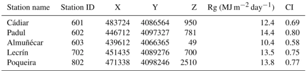
Table 1.UTM coordinates of the weather stations, measured daily global radiation and clearness index on the 20 November 2004.
Station name Station ID X Y Z Rg (MJ m−2day−1) CI
C´adiar 601 483724 4086564 950 12.4 0.69 Padul 602 446712 4097327 781 14.4 0.80 Almu˜n´ecar 603 439612 4066365 49 10.4 0.58 Lecr´ın 702 451435 4089276 700 13.5 0.75 Poqueira 802 471338 4098246 2510 13.8 0.77
as 802 in Fig. 1). Measurements of global radiation at station 802 were made with a Kipp and Zonen SP-Lite pyranometer, with a characteristic range of 0.4∼1.1 µm. The sensor was placed on a horizontal surface, partially surrounded by higher ground to the north but completely exposed to the south.
Even though the measurements at weather stations consti-tute a point source of information, for the purposes of these studies, those records can be assumed to constitute represen-tative average values for the cell on which they are located (Batll´es et al., 2008; Mart´ınez-Durb´an et al., 2009).
2.2 Calculation of solar radiation components including topographic effects
The topographic effects on solar radiation are mainly vari-ations in the illumination angle and shadowing from local horizons, the apparent intersection of the earth and the sky as seen by an observer in a certain direction. The local horizon information from the gridded data allows us to as-certain whether a given location at a as-certain sun position is shaded from direct sunlight by surrounding terrain and de-termines, at any location, the portion of the overlying hemi-sphere which is obscured by the terrain (Dozier et al., 1981; Dubayah, 1992). Thus, each hourly component, beam, dif-fuse and reflected radiation has been calculated separately to account for the topographic effects (Gonz´alez-Dugo et al., 2003) from the daily global radiation data measured at weather stations.
According to Essery and Marks (2007), despite the fact that since the availability of gridded data and powerful com-puters many efficient algorithms for calculating distributions of solar radiation over topographic grids have been devel-oped, all of them implement the same basic geometric princi-ples. Thus, the calculation of horizons in this study was made following the modification to the method by Dozier (1980), made more computationally efficient by Dozier et al. (1981) and Dozier and Frew (1990). They developed a simple and fast algorithm for the extraction of horizons from DEMs by comparing slopes between cells in a certain direction, and formulated the problem by determining the coordinates of the points which constitute the horizons in each cell. Then, by rotating the matrix and solving it in a one-dimensional way along each row as many times as the directions
consid-ered, they derived the horizons in the whole hemisphere for each cell in the DEM. In this study, eight directions were con-sidered in the calculation: the four cardinal points and their mid-way points.
2.2.1 Beam and diffuse component estimation on horizontal surfaces
The extraterrestrial radiation at any moment of time incident upon a horizontal surface located at an angle relative to the sun’s beams (Ro), is a function of the solar coordinates (the
zenith angle (θz)or its complementary angle, the sun
ele-vation angle (hs), and the solar azimuth (ψ)) and the solar
constant (ICS)corrected with the eccentricity factor (Eo)to
account for the changes in distance from the earth to the sun along the elliptical trajectory:
Ro=Eo·ICSsin(hs)=Eo·ICScos(θz) (1)
ICSwas fixed as 1367 Wm−2(Fr¨olich and Brusa, 1981) and
solar coordinates, which were calculated following the equa-tions in Iqbal (1983), are funcequa-tions of geographical latitude (φL), and solar declination (δ) in radians. For the solar decli-nation, the value at noon can be used as a constant daily value (Iqbal, 1983) and, as a medium-sized watershed, unique val-ues for latitude and longitude were considered, and, there-fore, a constant daily value of extraterrestrial solar radiation was obtained for the whole watershed.
In order to obtain the total amount of global radiation during one day (MJ m−2day−1), extraterrestrial radiation
(Eq. 1) must be integrated from sunrise to sunset. Thus, by assuming that the solar beam angle originates from the cen-ter of the solar disk, Eq. (1). was integrated following the expressions in Iqbal (1983) between the beginning and end-ing sun-hour angles when the sun’s beam first and last strikes the surface (Allen et al., 2006).
The basic procedure for the partition of daily global ra-diation into its components is the application of empirical correlations between the daily global radiation (Rg)and its diffuse component (Rd), and the ratio of daily global
radi-ation to extraterrestrial radiradi-ation (Ro), known as the daily
previously available correlations when applied locally for high-quality data recorded in Cyprus, and found that these correlations are location-independent. However, they devel-oped a specific correlation, which is more suitable for apply-ing in Mediterranean areas.
CI=RgRo (2)
RdRg=
0.992−0.0486CI CI≤0.1
0.954+0.734CI−3.806CI2+1.703CI3 0.1≤CI≤0.71
0.165 CI≥0.71
(3)
Beam daily solar radiation (Rb)can be obtained as the
dif-ference between global and diffuse radiation. Therefore, by applying Eq. (2), dailyRd andRb values (MJ m−2day−1)
can be estimated at each weather station with daily Rg
(MJ m−2day−1) available datasets. However, for the
spa-tial interpolation of daily beam and diffuse solar radiation, the lower scattering and absorption effects in high elevations, due to the lower air mass and vice versa, must be taken into account, especially with a quickly changed altitude (Yang et al., 2010). In this way, an atmospheric correction has to be performed pixel by pixel (Li et al., 2002).
The estimation of clear-sky solar radiation helps to eval-uate the effects of the atmospheric properties in a cloudless atmosphere. In this way, incident global daily radiation could be defined as being the product of the incident daily global radiation under clear sky conditions (Rgcs)and a cloudiness factor (fCIcl)that attenuatesRgcs.
Rg=Rgcs·fCIcl (4)
Thus, a theoretical clearness index for clear sky conditions (CIcs)could be defined as the ratio of global radiation under
clear sky conditions to extraterrestrial radiation (Rgcs/Ro),
In the literature there are numerous reviews and evaluations of the different models for the estimation of clear-sky solar radiation (Ineichen, 2006; Annear and Wells, 2007; Tham et al., 2009). In this study, the approximation of Ineichen and P´erez (2002) was applied based on its implementation simplicity. Thus,Rgcscan be obtained for each hour of the day from the sun elevation angle, the altitude in meters (z), the Linke turbidity factor (TL)and the air mass (AM) calcu-lated in terms of the height and solar elevation according to Kasten and Young (1989) andTL for air mass 2. However, even thoughTL can vary within a year (Mavromatakis and
Franghiadakis, 2007), a constant value of 2 was considered in this study as a first approximation.
CIcs=
Rgcs Ro
=a1·exp(−a2·AM·(fh1+fh2·(TL−1))) (5)
a1,a2,fh1andfh2 are empirical expressions that relate the
altitude of the station to the altitude of the atmospheric inter-actions (Rayleigh and aerosols). A detailed description can be found in Ineichen and P´erez (2002).
ReplacingRgcsin Eq. (4) by CIcs leads to Eq. (6), similar
to Suehrcke’s formulation (2000):
Rg=Ro·CIcs·fCIcl (6)
CI=CIcs·fCIcl (7)
Therefore, the clearness index (Eq. 7) can also be expressed as the combination of two factors, CIcs that shows the
in-fluence of the atmosphere over solar radiation in a cloudless atmosphere, andfCIcl, that decreases the incoming solar
ra-diation due to cloudiness effects. Eq. (7) constitutes the basis for the distributed computation of the CI in order to cal-culate the spatial fields of the different daily solar radiation components.
CIcs can be easily obtained at each cell and at an hourly
scale as it varies with the sun elevation angle and the height of the cell (Eq. 5), and, then, mean daily distributed values are calculated cell by cell. In addition, the daily CI values are calculated at each weather station from Eq. (1) with daily measured data, and from Eq. (7) with the mean daily values of CIcs at the cells where the weather stations are located,
the mean daily values of fCIcl at each station can be
ob-tained. Thus,fCIclvalues are spatially interpolated
follow-ing the inverse distance weighed (IDW) method, in order to distribute it throughout the watershed. This may appear to be an unrealistic simplification, but it is justified by the lack of more spatially distributed registering sites, which would al-low a better assessment of the spatial variation of cloudiness in the watershed. FromfCIcl and CIcs fields, daily global
radiation values (MJ m−2day−1) can be calculated (Eq. 6) at
cell scale and finally from Eq. (7) daily CI fields become available. Once daily global radiation and daily CI fields are obtained, the application of Eq. (3) is straightforward at the cell scale, and so distributed values of the daily dif-fuse and beam radiation components (MJ m−2day−1) can be
computed.
For the temporal downscaling of the solar radiation com-ponents, the application of hourly relations between hourly CI and hourly diffuse radiation values was initially consid-ered following previous works in the literature (Orgill and Hollands, 1977; Bugler, 1977; Erbs et al., 1982). However, the aim of this work was to provide a feasible method to include topographic effects on radiation at watershed scale, and the size and heterogeneity of the study site together with the lack of weather stations, which, unfortunately, are usual circumstances in many locations, make it unreasonable to spatially interpolate hourly CI values as the spatial distri-bution of diffuse and direct radiation shows a better corre-lation at a daily scale. Thus, a simpler approach is pro-posed so that once the daily values of each component are obtained for each cell, the hourly values (rb and rd, both
in (MJ m−2h−1)), are computed by distributing the daily
Finally, hourly values of beam and diffuse radiation on horizontal surfaces can then be transposed to give hourly radiation on tilted surfaces and the assessment of topographic effects as explained next.
2.2.2 Conversion from estimates on horizontal surfaces to tilted surfaces
Beam radiation
Under the isotropic assumption, hourly beam radiation on a surface of slopeβ and orientation γ (rb,βγ (MJ m−2h−1))
for a certain hour angle (ω) can be expressed in terms of the hourly beam radiation on an horizontal surface (rb), the
zenith angle (θz)and a new corrected zenith angle for the
sloping surface (θ) (Iqbal, 1983):
rb,βγ=rb cosθcosθz (8)
Therefore, for the calculation of hourly beam solar radia-tion on tilted surfaces, a correcradia-tion in the solar coordinates is necessary, so that the cosine of the zenith angle includes the effect of slope and orientation. This corrected zenith an-gle or illumination anan-gle (θ), function of the sun-earth-tilted surface geometrical relationship, can be obtained as (Iqbal, 1983; Allen et al., 2006):
cosθ=sinδ·(sinφL·cosβ−cosφL·sinβ·cosγ )+
cosδ·cosω·(cosφL·cosβ+sinφL·sinβ·cosγ )+
cosδ·sinβ·sinγ·sinω
(9)
Therefore, the main factors conditioning the fraction of beam radiation are not only the slope and aspect of the location rel-ative to its neighbors, but also the location of the sun relrel-ative to the slope at each time step. A certain location is receiving direct sunlight if none of the following situations are taking place:
– Self-shadowing due to its own slope: this takes place if the vector normal to the surface forms an angle greater than 90◦
with the solar vector (Gonz´alez-Dugo et al., 2003) (e.g. north-facing hill slope and 45◦
slope, sun in the south at 30◦
over the horizon). This situation is easy to calculate, as Eq. (7) yields a negative value.
– Shading cast by the nearby terrain: in this case, the sun is hidden by a local horizon. This case is more com-plex, since, unlike slope and orientation, it cannot be calculated with information restricted to the immediate neighborhood of a given point (Dozier et al., 1981). In order to express it mathematically, the term known as horizon angle in a certain directionφ,H8, is introduced
as the angle between the normal to the surface and the line joining this point or grid in the DEM with another point in the same direction high enough to block so-lar radiation. Thus, shading by the surrounding terrain will occur for each time step if the illumination angle is greater than the horizon angle in that direction.
Diffuse radiation
Topography influences the diffuse component by modifying the portion of the overlying hemisphere visible at a certain point. The computation of scattered and reflected radiation amounts from the atmosphere to the slopes is rather compli-cated, owing to their non-isotropic nature. A common as-sumption made is that the diffuse component of solar radi-ation (sky light) has an isotropic distribution over the hemi-spherical sky. However, the non-isotropic character of dif-fuse radiation fields (maximum intensities near the sun and the horizons, minimum intensities in the direction normal to that of the sun, etc.) makes the simplified assumption suf-ficiently unrealistic to introduce errors into calculations of the energy incident on sloping surfaces (Temps and Coulson, 1977). Nevertheless, following the ideas of Kondratyev and Manolova (1960), who concluded that the isotropic approx-imation is sufficient for practical purposes (Klutcher, 1979), the isotropic assumption will prevail in this study with the portion of overlying hemisphere visible at each cell as the main factor controlling this component. Thus, the hourly diffuse radiation (rd,βγ(MJ m−2h−1)) on a surface of slope
βand orientationγ, is:
rd,βγ=rd·SVF (10) where the sky view factor, SVF, is the ratio between the diffuse component at one given point and that on an un-obstructed horizontal surface, so that it corrects the in-coming radiation incident on a flat surface to radiation over a sloping and possibly obstructed surface (Dubayah, 1992). Under the assumption of an isotropic sky, a con-stant value for the SVF can be expressed analytically in terms of the different horizons in each direction considered, as (Dozier and Frew, 1990):
SVF=
8 X
φ=1
cosβ·sin2Hφ+ sinβ·cosγ Hφ−sinHφcosHφ(11)
Reflected radiation
Albedo refers to the global reflectance of the surface to solar radiation. Both albedo and topography can vary over short distances, and their interaction can lead to a wide variabil-ity in global solar radiation on a scale of meters (Dubayah, 1992). Reflected radiation (rr,βγ(MJ m−2h−1)) can be
com-puted following the ideas of Dozier and Frew (1990) from:
rr,βγ=ρ· (1+cosβ) 2
−SVF
Landsat-5 and Landsat-7 satellites during the study period. After the images had been properly corrected and their re-flectivity values extracted, albedo values were obtained at the cell scale through the method proposed by Brest and Goward (1987) and interpolated for the whole time lapse on a daily basis.
Global radiation
Global radiation at an hourly scale at each cell (rg
(MJ m−2h−1)) was obtained as the sum of each component
at an hourly scale once: (1) direct radiation had been cor-rected by self-shadowing and shadows cast by nearby terrain; (2) diffuse sky radiation included the portion of the overlying hemisphere that could be obstructed by nearby terrain, and (3) direct and diffuse radiation reflected by nearby terrain to-wards the location of interest had been calculated from both corrected components (Dubayah, 1994). And finally, daily global radiation (Rg(MJ m−2day−1)) was calculated by
in-tegration of the hourly global radiation estimates cell by cell. For the purposes of computer simulation programs, which handle vast amounts of data, the algorithm was implemented in Matlab during the trials, and, finally, in C++ to obtain a sufficiently fast computation, considering all the processes involved at a cell scale. Also, some of the assumptions that could appear to be quite unrealistic due mainly to the scarcity of data, are intended to achieve a compromise between a suf-ficiently representative distributed approximation and a high-speed processing algorithm that can be run on a desktop PC, from the comparison with measured data and simpler inter-polation techniques. Finally, through the use of daily sam-ples, the availability of data is enhanced as not many hourly records are needed; this allows the use of the algorithm in mountainous areas which lack a high frequency monitoring network, so common in many other areas.
2.3 Evaluation of the topographic effects on solar radiation fields on reference evapotranspiration estimates
The choice of a method for the calculation of ET0depends on
numerous factors. The energy available at the soil surface is the first control of the process, so the estimation of this factor from accessible data sometimes conditions the method (Shut-tleworth, 1993). In this study, the ASCE-Penman Monteith equation (Eq. 13) was applied for the estimation of evapo-transpiration over a reference surface (Allen et al., 1998):
ETASCE0 =
0.4081(Rn−G)+γT+273.16Cn u2(es−ea)
1+γ (1+Cdu2)
(13) where ETASCE0 is the reference evapotranspiration during a certain time step (mm/1t);1the slope of the vapor pressure-temperature-curve saturation calculated at mean air temper-ature (kPa/◦C);γ the psychrometric constant (kPa/◦C);R
n
andGthe net radiation (combination of net short-wave and net long-wave radiation) and soil heat fluxes, respectively, both in mm/1twater equivalent;eaandesthe actual and sat-uration vapor pressure (kPa), respectively;T the daily mean air temperature (◦
C) andu2the wind speed, both measured at a height of 2 m above the soil surface (m/s). Finally,Cd
andCn are resistance coefficients which vary with the
ref-erence crop, temporal time-step and, in the case of hourly time-steps, with daytime and night time. Here, the reference surface defined in the FAO PM equation was considered so that for daily time steps the values ofCdandCnwere 900 and
0.34, respectively (Allen et al., 1998; Gavil´an et al., 2008). The calculation of some of the variables involved in the ASCE-PM equation can be found in detail depending on the input data available in Allen et al. (1998). Sax-ton (1975) found out that the variable to which the equa-tion is most sensitive is net radiaequa-tion, here expressed as the sum of net short-wave radiation, Rns, and net long-wave radiation,Rnl, at the Earth’s surface. Net daily short-wave radiation (Eq. 14) on the soil surface, as the dif-ference between incident and reflected radiation, can be expressed in terms of the albedo of the surface, α (0.23 for the reference surface) and the predicted incoming so-lar global radiation, Rg (MJ m−2day−1). In the same
way, the net long-wave radiation was approximated by Eq. (15) where εatm is the atmospheric emissivity, T (K)
the mean air temperature andσ Stefan-Boltzmann’s constant (4.903×10⁻⁹MJ K−4m−2day−1). The atmospheric
emis-sivity was calculated through a parametric expression by Herrero et al. (2009) based on near-surface measurements of solar radiation and relative humidity, valid for the local con-ditions of the study area. Therefore, the expression for net long-wave radiation remains as previously done by other au-thors (Doorenbos and Pruitt, 1977; Allen, 1986; Allen et al., 1998) as a modification to Stefan-Boltzmann’s law due to the absorption and downward radiation from the sky. Thus, the product of the Stefan-Boltzmann’s constant and the mean air temperature to the fourth power is multiplied by a cloudiness and an air humidity factor (Allen et al., 1998; Donatelli et al., 2006), both factors included in this study in the termεatm
and so, together with the mean air temperature, they consti-tute the only inputs to the equation.
Rns=(1−a)Rg (14)
Rnl≈(εatm−1)·σ·T4 (15)
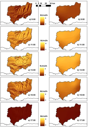
Fig. 2. Hourly global radiation(a)topographically corrected vs. (b)IDW interpolated (20 November 2004).
3 Results and discussion
In order to run the proposed set of algorithms at the water-shed scale, hourly global radiation was calculated from each 30×30 m2cell of the DEM in the study area for the period comprised between 4 November 2004 and 2 July 2010.
The results are organized into three sections. Firstly, com-parisons of the results obtained through the topographic radi-ation algorithm previously exposed with those derived from a classical interpolation technique are shown. Secondly, the suitability of the results at different temporal scales is presented through its comparison with field measurements, proving the accuracy of the estimated values for hydrologi-cal distributed modeling. Finally, in order to address the hy-drologic importance of using topographically corrected solar radiation fields over uniform values obtained through clas-sical interpolation techniques, the influence of both estima-tions as inputs to reference evapotranspiration computaestima-tions is evaluated.
Table 2. Maximum, minimum, mean and standard deviation (MJ m−2h−1) of hourly solar radiation estimates in the watershed on the 20 November 2004 obtained by the topographic approxima-tion and IDW to the values measured at staapproxima-tions with hourly avail-able datasets (601, 602, 603 and 802).
Topographic (MJ m−2h−1) IDW (MJ m−2h−1)
Hour Min Max Mean σ Min Max Mean σ
08:00 0.03 0.83 0.18 0.09 0.14 0.29 0.19 0.04 09:00 0.06 2.81 0.85 0.54 0.39 1.21 0.92 0.18 10:00 0.06 3.51 1.43 0.72 0.92 1.91 1.56 0.20 11:00 0.06 3.78 1.84 0.72 1.26 2.38 2.00 0.24 12:00 0.07 3.88 2.05 0.71 1.48 2.61 2.23 0.26 13:00 0.07 3.86 2.05 0.70 1.55 2.64 2.23 0.27 14:00 0.06 3.74 1.83 0.70 1.37 2.43 2.00 0.26 15:00 0.06 3.46 1.40 0.68 0.92 1.95 1.55 0.23 16:00 0.06 2.69 0.81 0.50 0.43 1.20 0.92 0.16 17:00 0.03 0.61 0.15 0.07 0.12 0.21 0.18 0.02
3.1 Topographic corrections v. classic interpolation techniques on solar radiation estimates
At the first stage, topographic information was derived from the DEM (Fig. 1) in the study area. Slope and orientation maps were obtained and the horizons for each cell were cal-culated as stated before. Once these parameters are available for a certain area they can be used in subsequent executions as they are considered to be independent of the time of year. In order to compare the results obtained through the to-pographic algorithm with those of classic interpolation tech-niques at an hourly scale, a reference day was selected. This date, 20 November 2004, was chosen as it was cloudless and it had not rained for several days. This condition is very important for the albedo estimation from remote sens-ing images, as the presence of moisture in the environment influences the quality of the estimates, and, therefore, con-secutively dry days are most suitable for an accurate perfor-mance. Moreover, remote sensing images were available for this date, and, therefore, the errors due to the temporal inter-polation of albedo values were minimized.
The hourly sequence of global radiation, as the sum of each component at an hourly scale once each component has been properly corrected, is shown in Fig. 2a, where the spa-tial gradient in hourly global radiation is evident. On the whole, it can be seen that the locations receiving more ra-diation are those in the highest part of the watershed, with a south-facing orientation that remains unobstructed during most of the hours of daylight.
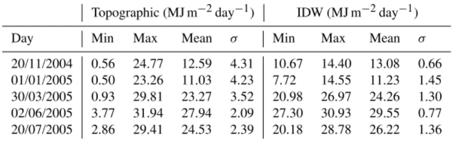
Table 3.Maximum, minimum, mean and standard deviation (MJ m−2day−1) of daily solar radiation estimates in the watershed on selected days obtained by the topographic approximation and IDW to the values measured at stations with daily available datasets (601, 602, 603, 702 and 802).
Topographic (MJ m−2day−1) IDW (MJ m−2day−1)
Day Min Max Mean σ Min Max Mean σ
20/11/2004 0.56 24.77 12.59 4.31 10.67 14.40 13.08 0.66 01/01/2005 0.50 23.26 11.03 4.23 7.72 14.55 11.23 1.45 30/03/2005 0.93 29.81 23.27 3.52 20.98 26.97 24.26 1.30 02/06/2005 3.77 31.94 27.94 2.09 27.30 30.93 29.55 0.77 20/07/2005 2.86 29.41 24.53 2.39 20.18 28.78 26.22 1.36
maximum values in the watershed, as well as the mean and standard deviation of the hourly estimates through both dis-tributed computations, are shown in Table 2. It can be seen that even though the mean values in the watershed present a slightly similar order of magnitude, differences in the stan-dard deviation, maximum and minimum values between both methodologies were remarkable in every hour of the day. From contrasting results between Fig. 2a and b, not only was a huge difference visible in the distributed values of the variable cell by cell, but also noticeable was the wider range of global values in the watershed, when topographic factors are taken into account, as shown by the maximum, minimum and standard deviation values in Table 2. In this latter case, extreme values, far exceeding the measured values, repre-sent extreme conditions, such as high areas remaining unob-structed most of the daytime and sometimes receiving almost double the values obtained through interpolation of the data recorded at the stations or, at the other end of the scale, val-leys that receive minimal or even zero quantities of solar ra-diation, due to the configuration of the surrounding terrain. The higher maximum hourly estimates and standard devia-tion values, as well as the lower minimum hourly estimates obtained by the topographic approximation (Table 2), quan-tify this fact. As a result, processes such as evaporation or snowmelt, which rely heavily on solar radiation, can be mis-calculated under a wide range of conditions, such as overes-timations in areas obstructed by nearby terrain or underesti-mations in the upper and exposed regions of the watershed, among others.
Hourly values can be aggregated in each cell at the re-quired temporal scale. In this way, Fig. 3 represents the spatial distribution of daily global radiation on 20 Novem-ber 2004 estimated through the topographic algorithm (Fig. 3a) and from IDW (Fig. 3b), respectively. Again, the same conclusions can be drawn as at an hourly time step, since maximum and minimum values found in the watershed considering topographic effects are quite different to those obtained through IDW and the daily values recorded at the weather stations (Table 1). Thus, we found differences of
Fig. 3. Daily global radiation (20 November 2004)(a) topograph-ically corrected vs.(b)IDW interpolated, and annual global radia-tion (1 September 2004–31 August 2005)(c)topographically cor-rected vs.(d)IDW interpolated.
as much as an extra 42% in the estimated daily values com-pared with those obtained through spatial interpolation with-out consideration of topography, predominantly on the swith-outh- south-facing hillsides in the northern part of the watershed, and un-derestimations of up to−1800 % in certain cells obstructed most of the daytime, with a mean difference of−4% in the whole watershed. In addition, the same computation was ap-plied for different cloudless days when there were remote sensing images available (1 January 2005, 30 March 2005, 2 June 2005 and 20 July 2005). Table 3 again shows the same general trend in the basic statistics (absolute minimum and maximum values and the mean and standard deviation of the daily estimates in the watershed) for all the days considered: proximity in the mean values obtained by both methodolo-gies, but considerable differences in the extreme values and in the standard deviation, as stated before.
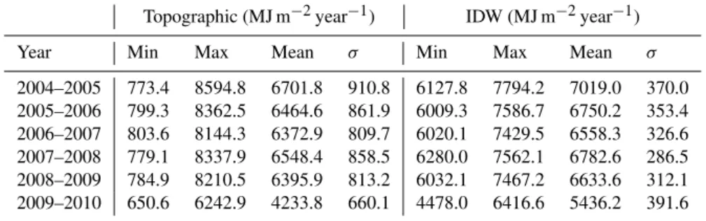
Table 4.Maximum, minimum, mean and standard deviation (MJ m−2year−1) of annual solar radiation estimates in the watershed obtained by the topographic approximation and IDW to the annual accumulated values measured at stations with daily available datasets (601, 602, 603, 702 and 802).
Topographic (MJ m−2year−1) IDW (MJ m−2year−1)
Year Min Max Mean σ Min Max Mean σ
2004–2005 773.4 8594.8 6701.8 910.8 6127.8 7794.2 7019.0 370.0 2005–2006 799.3 8362.5 6464.6 861.9 6009.3 7586.7 6750.2 353.4 2006–2007 803.6 8144.3 6372.9 809.7 6020.1 7429.5 6558.3 326.6 2007–2008 779.1 8337.9 6548.4 858.5 6280.0 7562.1 6782.6 286.5 2008–2009 784.9 8210.5 6395.9 813.2 6032.1 7467.2 6633.6 312.1 2009–2010 650.6 6242.9 4233.8 660.1 4478.0 6416.6 5436.2 391.6
Fig. 4.Observed (Rgo), and predicted (Rgp)global daily radiation (MJ m−2day−1) at station 702 and 802 for the evaluation period (4 November 2004–2 July 2010).
and d) resulted in a mean excess of 323.75 MJ m−2year−1
with a standard deviation of 860 MJ m−2year−1 when
ap-plying IDW over the topographic computation and extreme differences of the same order of magnitude as at the daily time step. The same comparison for the rest of the hydrolog-ical years of the study period can be seen in Table 4, where the last year is incomplete as data from July and August 2010 were not yet available. Once again, higher extremes and stan-dard deviation values through the topographic approximation were obtained. However, unlike at hourly and daily time scales, the accumulation of differences at annual scale leads to a certain variability in the mean values of annual radiation estimates in the watershed between both methodologies for every hydrological year (200–300 MJ m−2year−1).
Fig. 5. Extraterrestrial solar radiation (Ro), observed (Rgo), and predicted (Rgp)global radiation (MJ m−2day−1) at station 802 for the evaluation period (4 November 2004–2 July 2010).
3.2 Validation of topographic corrections
The radiation values generated from datasets of stations 601, 602 and 603 were compared to the radiation measurements at stations 802 and 702 and the agreement between gen-erated and measured data was evaluated through 1:1 lines. The period considered in the evaluation was determined by the availability of data in the weather station 802, which in-cluded almost six hydrological years, from 4 November 2004 to 2 July 2010. However, even though station 702 presents sparse measurements from the beginning 2008 until nowa-days, the adjustment for the rest of the period is shown.
measured and generated values appears to be more related to the direct interpolation of the cloudiness factor and to the fact that in those periods the availability of remote sensing im-ages for an accurate estimation of albedo was more limited than to the assumptions of the topographic approximation ap-plied in this study. Also, the low RMSE values as well as the proximity ofR2 estimates to 1 at both stations demonstrate the ability of the topographic approximation to estimate so-lar radiation in high elevations even when the only available datasets come from weather stations that are located at a rel-atively low elevation compared to the mean height of the watershed. To conclude, the accuracy of predicted hourly values was assessed in station 802, where measurements at this time scale were available. Despite the scattering effect observed in Fig. 6, which shows the agreement between pre-dicted (rgp)and measured (rgo)hourly values for the evalua-tion period, we can say that the algorithm reasonably predicts the observed data with aR2of 0.87, especially considering the time scale and some of the assumptions of the algorithm, which at this time step might appear to be rather simplistic. Therefore, the installation of a denser monitoring network provided with solar devices recording hourly direct and dif-fuse radiation data may improve the results. Firstly, it would provide the spatial scheme required for the spatial interpola-tion of hourly values. Secondly, it would allow the inclusion of more factors for the spatial distribution of the fCIcl as
previously suggested. Finally, the derivation of hourly corre-lations between the hourly diffuse radiation and the CI would be reasonable in the study area. To sum up, the possibility of working at finer scales would be the ideal as the geometrical relationships involved in the calculation of extraterrestrial ra-diation are continuous in time. However, independently of this continuous nature of extraterrestrial radiation, the time scale of the computation of the incoming solar radiation is determined by the temporal frequency of the monitoring net-work. Nevertheless, the calculations with aggregated hourly values at higher temporal scales such as the daily time step showed the same degree of detail as at the hourly time scale (R2around 0.9).
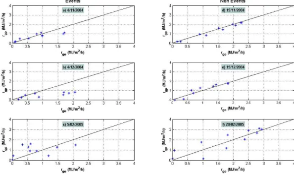
Finally, since cloudless skies are required for an accurate characterization of the albedo from remote sensing images, the results at an hourly time step were analyzed consider-ing this effect. Thus, two different atmospheric situations in terms of the occurrence of rainfall are defined as an in-dicator of the cloudiness in the atmosphere: events (when it rains somewhere in the watershed) and non-events (periods between events). Figure 7 represents hourly values for event days on the left-hand side (a, b, c) and non-events on the right (d, e, f).
Table 5 shows different linear fits for each day represented in Fig. 7 and its calculated R2 values. As was expected, the predicted values were much better for cloudless skies or non-events when acceptableR2 values were obtained even when forcing the adjustment to reach the origin. However, as with daily values, the algorithm slightly underestimated the
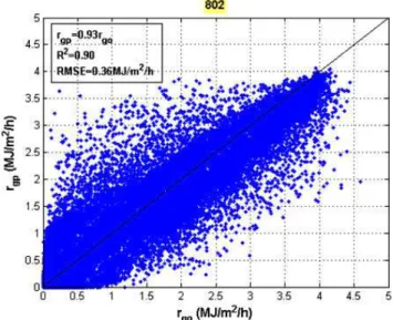
Fig. 6.Observed (rgo), and predicted (rgp)global hourly radiation (MJ m−2h−1) at station 802 for the evaluation period (4 Novem-ber 2004–2 July 2010).
Table 5. Linear fits of observed (rgo), and predicted (rgp)global hourly radiation (MJ m−2h−1) at station 802 for certain dates.
Equation type rgp=a·rgo rgp=a·rgo+b a R2 a b R2
Events
a) 4/11/2004 0.77 0.58 0.55 0.26 0.75 b) 4/12/2004 0.42 0.47 0.29 0.20 0.61 c) 5/02/2005 0.92 0.05 0.36 0.71 0.19
Non events
d) 15/11/2004 0.95 0.97 0.98 −0.04 0.97 e) 15/12/2004 1.05 0.89 1.03 0.04 0.89 f) 20/02/2005 0.99 0.73 0.88 0.32 0.76
observed hourly values, which could be improved with the consideration of the variation in cloudiness at an hourly time step and a more detailed study of the temporal variation in the albedo in the area. In any case, the worst fits obtained in situations when events occur are expected to be more closely related to the separation of the different components in the global radiation value than to the topographic interpolation process.
Fig. 7.Scatter plots of observed (rgo), and predicted (rgp)global hourly radiation (MJ m−2h−1) at station 802 for certain dates.
Fig. 8.Daily ET0with global radiation (20 November 2004)(a) to-pographically corrected vs.(b)IDW interpolated, and annual ET0 with global radiation (1 September 2004–31 August 2005)(c) topo-graphically corrected vs.(d)IDW interpolated.
days constitute a higher rate than cloudy days associated with situations when events occur in a Mediterranean area like the present study site: in this case, around 75% of clear sky days for the evaluation period.
3.3 Influence of the inclusion of topographic corrections on hydrological variables: ET0
Finally, a distributed computation of ET0was applied for the
same reference day of Sect. 3.1 (Fig. 8a) and the hydrological year 2004 (Fig. 8c) (1 September 2004 to 31 August 2005) once all the variables involved in the ASCE-PM equation had been spatially derived including topographic effects. Also, the ASCE-PM equation was computed with solar radiation surfaces obtained through IDW of the data recorded at the stations as inputs to the equation (Fig. 8b and d) in order to prove the importance of solar radiation fields which in-clude topographic corrections. Again, in Fig. 8a and c, not only the apparent spatial variability of ET0estimates cell by
cell which follows the topographic gradient can be seen, but also a wider range of values in the watershed than with IDW-interpolated solar radiation fields as inputs (Fig. 8b and d). Besides, in this latter case, ET0 estimates in the watershed
appear to be more influenced by the spatial distribution of other variables than by solar radiation (e.g. temperature in Fig. 8b). This spatial variability is quantified in terms of the basic statistics of the distributed estimates through both methodologies for the rest of the reference days and hydro-logical years, respectively (Table 6 and 7). Again, mean values of the same order of magnitude at daily scale but very extreme values for the maximum and minimum es-timates when using the topographic corrected solar radia-tion, and, therefore, higher standard deviation values than with IDW-interpolated solar radiation fields as inputs (Ta-ble 6) can be noted. However, as annual estimates of ET0
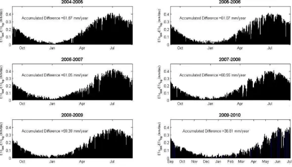
Fig. 9. Daily differences between mean ET0 estimates at watershed scale with global radiation IDW interpolated and topographically corrected (ET0IDW–ET0Top).
Table 6. Maximum, minimum, mean and standard deviation (mm/day) of daily evapotranspiration estimates in the watershed on selected days with global radiation topographically corrected and IDW interpolated.
Topographic (mm/day) IDW (mm/day)
Day Min Max Mean σ Min Max Mean σ
20/11/2004 0.15 3.60 1.68 0.74 0.90 2.20 1.71 0.26 01/01/2005 0.10 3.30 1.35 0.70 0.60 1.90 1.36 0.24 30/03/2005 0.20 5.42 3.89 0.61 3.30 4.80 4.07 0.22 02/06/2005 0.20 5.64 4.42 0.43 4.20 5.60 4.77 0.25 20/07/2005 0.90 7.12 5.46 0.74 3.30 7.10 5.78 0.64
accumulation of the differences between both methodolo-gies at finer scales becomes apparent in the mean annual values (around 60 mm/year) at watershed scale from both methodologies (Table 7).
Finally, Fig. 9 represents the mean daily difference at wa-tershed scale for each hydrological year of ET0estimations
when using IDW-interpolated and topographically-corrected solar radiation fields. It can be seen that there is a general overestimation with IDW-interpolated solar radiation fields every day of the year. Also, these overestimations follow the temporal pattern of solar radiation, and so the biggest differences (0.4 mm/day) take place in summer, when the im-portance of ET0in the water balance is greater. Considering
the mean statistics of the difference between both computa-tions on an annual basis, a mean excess of 61 mm/year and a standard deviation of 142 mm/year in ET0estimations when
using IDW-interpolated solar radiation fields were obtained for the study period. These differences in an area where the
mean annual rainfall varies from 450 mm/year on the coast to 800 mm/year on the highest peaks may constitute a con-siderable source of error in the water balance when apply-ing distributed hydrological models for the management and planning of water resources.
4 Conclusions
Difficulties are sometimes encountered in utilizing available solar radiation data, since they consist primarily of total (di-rect plus diffuse) radiation only, and a knowledge of the val-ues for each component is often required, especially for the consideration of topographic effects as they affect each com-ponent differently.
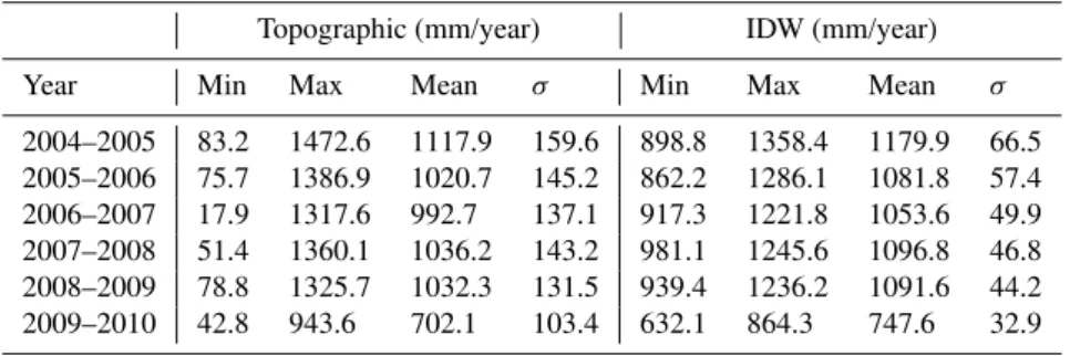
Table 7.Maximum, minimum, mean and standard deviation (mm/year) of annual evapotranspiration estimates in the watershed on selected days with global radiation topographically corrected and IDW interpolated
Topographic (mm/year) IDW (mm/year)
Year Min Max Mean σ Min Max Mean σ
2004–2005 83.2 1472.6 1117.9 159.6 898.8 1358.4 1179.9 66.5 2005–2006 75.7 1386.9 1020.7 145.2 862.2 1286.1 1081.8 57.4 2006–2007 17.9 1317.6 992.7 137.1 917.3 1221.8 1053.6 49.9 2007–2008 51.4 1360.1 1036.2 143.2 981.1 1245.6 1096.8 46.8 2008–2009 78.8 1325.7 1032.3 131.5 939.4 1236.2 1091.6 44.2 2009–2010 42.8 943.6 702.1 103.4 632.1 864.3 747.6 32.9
mountainous Mediterranean environments. The interpolation is managed through linear interpolation of the cloudiness ef-fects and the variation of the CI with elevation as a clue to mean daily radiation, plus topographic properties geometri-cally related to the sun’s position at hourly intervals. These calculations are easy to reproduce from standard weather sta-tion datasets. The significant incidence of topography on the values of global solar radiation throughout the watershed has been demonstrated by the results of the topographic so-lar radiation algorithm proposed. In this sense, differences of as much as an extra 42% in the estimated daily values compared with those obtained through spatial interpolation without consideration of topography, and underestimations of up to−1800% in certain cells obstructed most of the day-time were found. This affects the modeling of the slow but thorough drying out of the watershed during periods between events and the modeling of the snowmelt in the highest areas, among other processes.
The simulated results fit the measured values of global ra-diation at the 2510 m high monitoring point established for this work really well, with a correlation of 0.93 for daily val-ues, and a RMSE of 2 MJ m−2day−1, that confirms the
va-lidity of the assumptions made in the algorithm, as the pvious paragraphs have justified. However, the simulated re-sults constitute a further approach to the accurate character-ization of the spatial distribution of hourly global radiation values in mountainous areas with scant data recording sites. On-going work will develop a further approach, and test the inclusion of additional corrective terms in the cloudiness factor through the establishment of two additional weather stations equipped with pyranometers at points with an in-creasing height above sea-level and distance from the sea.
The importance of considering the topographic gradients in the spatial distribution of solar radiation for the study of hydrological processes in which this variable plays a cru-cial role became evident against ET0 estimates with solar
radiation fields obtained through classical interpolation tech-niques of data recorded at weather stations. Thus, a mean excess of 61 mm/year was found with IDW-interpolated so-lar radiation fields as inputs to the ASCE-PM equation with the highest overestimations taking place in summer periods.
Acknowledgements. This work was funded by the Andalusian Water Institute in the project Pilot study for the integral man-agement of the Guadalfeo river watershed and by the Regional Innovation, Science and Enterprise Ministry grant for PhD training in Andalusian Universities and Research Centers.
Edited by: X. Li
References
Aguilar, C.: Scale effects in hydrological processes. Application to the Guadalfeo river watershed (Granada). PhD Thesis. Uni-versity of C´ordoba, http://www.cuencaguadalfeo.com/archivos/ Guadalfeo/Tesis/TesisCris en.pdf, last access: 5 April 2010, 2008.
Allen, R. G.: A Penman for all seasons, J. Irrig. Drain. Eng. ASCE., 112, 348–368, 1986.
Allen, R. G., Pereira, L. S., Raes, D., and Smith, M.: Crop evapo-transpiration, guidelines for computing crop water requirements, Irrig. and Drain. Pap., 56. U.N. Food and Agric. Organ., Rome, 1998.
Allen, R. G., Trezza, R., and Tasumi, M.: Analytical integrated functions for daily solar radiation on slopes, Agric. For. Meteo-rol., 139, 55–73, 2006.
Annear, R. L. and Wells, S. A.: A comparison of five models for estimating clear-sky solar radiation, Wat. Resour. Res., 43, W10415, doi:10.1029/2006WR005055, 2007.
Antonic, O.: Modelling daily topographic solar radiation without site-specific hourly radiation data, Ecol. Modelling, 113, 31–40, 1998.
Arnold, J. G., Srinivasan, R., Muttiah, R. S., and Williams, J. R.: Large area hydrologic modelling and assessment-Part I: model development, J. Amer. Water Res. Assoc., 34, 73–89, 1998. Batlles, J., Bosch, J. L., Tovar-Pescador, J., Mart´ınez-Durb´an, M.,
Ortega, R., and Miralles, I.: Determination of atmospheric pa-rameters to estimate global radiation in areas of complex topog-raphy: Generation of global irradiation map, Energ. Convers. Manage., 49, 336–345, 2008.
Bingner, R. L. and Theurer, F. D.: AnnAGNPS Technical Processes. USDA-ARS. National Sedimentation Laboratory, 2003. Brest, C. L. and Goward, S. N.: Deriving surface albedo
Bugler, J. W.: The determination of hourly insolation on an inclined plane using a diffuse irradiance model based on hourly measured global radiation insolation, Sol. Energy, 19, 477–491, 1977. Chen, R., Kang, E., Ji, X., Yang, J., and Wang, J.: An hourly
so-lar radiation model under actual weather and terrain conditions: A case study in Heihe river watershed, Energy, 32, 1148–1157, 2007.
Collares-Pereira, M. and Rabl, A.: The average distribution of solar radiation – Correlations between diffuse and hemispherical and between daily and hourly insolation values, Sol. Energy, 22, 155– 164, 1979.
Cronshey, R. G. and Theurer, F. D.: AnnAGNPS-Non-Point Pol-lutant Loading Model, in: Proceedings First Federal Interagency Hydrologic Modeling Conference, 19–23 April 1998, Las Vegas, NV, 1–9 to 1–16, 1998.
D´ıaz, A.: Temporal series of vegetation for a distributed hy-drological model. Master Thesis, University of C´ordoba, http://www.cuencaguadalfeo.com/archivos/Guadalfeo/Libros/ TFM Adolfo%20D%C3%ADaz.pdf, last access: 5 April 2010, 2007 (in Spanish).
Diodato, N. and Bellocchi, G.: Modelling solar radiation over com-plex terrains using monthly climatological data, Agric. For. Me-teorol., 144, 111–126, 2007.
Donatelli, M., Bellocchi, G., and Carlini, L.: sharing knowledge via software components: Models on reference evapotranspiration, Europ. J. Agronomy, 24, 186–192, 2006.
Doorenbos, J. and Pruitt, W. O.: Guidelines for predicting crop wa-ter requirements, Irrig. and Drain. Pap., 24. U.N. Food and Agric. Organ., Rome, 1977.
Dozier, J.: A clear-sky spectral solar radiation model for snow-covered mountainous terrain, Wat. Resour. Res., 16, 709–718, 1980.
Dozier, J., Bruno, J., and Downey, P.: A faster solution to the hori-zon problem, Comp. Geosci., 7, 145–151, 1981.
Dozier, J. and Frew, J.: Rapid calculation of terrain parameters for radiation modeling from digital elevation data, IEEE Trans. Geosci. Remote Sens., 28, 963–969, 1990.
Dubayah, R. C.: Estimating net solar radiation using Landsat The-matic Mapper and digital elevation data, Wat. Resour. Res., 28, 2469–2484, 1992.
Dubayah, R. C.: Modeling a solar radiation topoclimatology for the Rio Grande river watershed, J. Veg. Sci., 5, 627–640, 1994. Dubayah, R. and van Katwijk, V.: The topographic distribution of
annual incoming solar radiation in the Rio Grande river basin, Geoph. Res. Let., 19, 2231–2234, 1992.
Erbs, D. G., Klein, S. A., and Duffie, J. A.: Estimation of the diffuse radiation fraction for hourly, daily and monthly average global radiation, Sol. Energy, 28, 293–302, 1982.
Essery, R. and Marks, D.: Scaling and parametrization of clear-sky solar radiation over complex topography, J. Geophys. Res., 112, D10122, doi:10.1029/2006JD007650, 2007.
Flint, A. L. and Childs, S. T.: Calculation of solar radiation in mountainous terrain, Agric. For. Meteorol., 40, 233–249, 1987. Fr¨ohlich, C. and Brusa, R. W.: Solar radiation and its variation in
time, Solar Phys., 74, 209–215, 1981.
Garen, D. and Marks, D.: Spatially distributed energy balance snowmelt modelling in a mountainous river watershed: estima-tion of meteorological inputs and verificaestima-tion of model results, J. Hydrol., 315, 126–153, 2005.
Gavilan, P., Est´evez, J., and Berengena, J.: Comparison of standard-ized reference evapotranspiration equations in southern Spain, J. Irrig. Drain. Eng., 134, 1–12, 2008.
Gonz´alez-Dugo, M. P., Chica-Llamas, M. C., and Polo-G´omez, M. J.: Modelo topogr´afico de radiaci´on solar para Andaluc´ıa, in: XXI Congreso Nacional de Riegos, M´erida, 53–55, 2003. Graham, D. N. and Butts, M. B.: Flexible, integrated watershed
modelling with MIKE SHE, in: Watershed Models, edited by: Singh, V. P. and Frevert, D. K., CRC Press, Boca Raton, 245– 272, 2005.
Herrero, J.: Modelo f´ısico de acumulaci´on y fusi´on de la nieve. Aplicaci´on a Sierra Nevada (Espa˜na). PhD Thesis, University of Granada, http://www.ugr.es/∼herrero, last access: 5 April 2010,
2007 (in Spanish).
Herrero, J., Aguilar, C., Polo, M. J., and Losada, M.: Mapping of meteorological variables for runoff generation forecast in distributed hydrological modeling., in: Proceedings, Hydraulic Measurements and Experimental Methods 2007 (ASCE/IAHR), Lake Placid, NY, 606–611, 2007.
Herrero, J., Polo, M. J., Mo˜nino, A., and Losada, M.: An energy balance snowmelt model in a Mediterranean site, J. Hydrol., 271, 98–107, 2009.
Ineichen, P.: Comparison of eight clear sky broadband models against 16 independent data banks, Sol. Energy, 80, 468–478, 2006.
Ineichen., P. and P´erez, R.: A new airmass independent formulation for the Linke Turbidity coefficient, Sol. Energy, 73, 151–157, 2002.
Iqbal, M.: Prediction of hourly diffuse radiation from measured hourly global radiation on a horizontal surface, Sol. Energy, 24, 491–503, 1980.
Iqbal, M.: An introduction to solar radiation, Academis Press Canada, Ontario, 1983.
Jacovides, C. P., Hadjioannou, L., Pashiardis, S., and Stefanou, L.: On the diffuse fraction of daily and monthly global radiation for the island of Cyprus, Sol. Energy, 56, 565–572, 1996.
Kambezidis, H. D., Psiloglou, B. E., and Gueymard, C.: Measure-ments and models for total solar irradiance on inclined surface in Athens, Greece, Sol. Energy, 53, 177–185, 1994.
Kasten, F. and Young, A. T.: Revised optical air mass tables and approximation formula, App. Optics., 28(22), 4735–4738, 1989. Klutcher, T. M.: Evaluation of models to predict insolation on tilted
surfaces, Sol. Energy, 23, 111–114, 1979.
Kondratyev, K. J. and Manolova, M. P.: The radiation balance on slopes, Sol. Energy, 4, 14–19, 1960.
Li, X., Koike, T., and Cheng, G. D.: Retrieval of snow reflectance from Landsat data in rugged terrain, Ann. Glaciol., 34, 31–37, 2002.
Liu, B. Y. H. and Jordan, R. C.: The interrelationship and character-istic distribution of direct, diffuse and total solar radiation, Sol. Energy, 4, 1–19, 1960.
Mart´ınez-Durb´an, M., Zarzalejo, L.F., Bosch, J. L., Rosiek, S., Polo, J., and Batlles, F. J.: Estimation of global daily irradia-tion in complex topography zones using digital elevairradia-tion models and meteosat images: Comparison of the results, Energ. Convers. Manage., 50, 2233–2238, 2009.
Millares, A.: Integraci´on del caudal base en un modelo distribuido de cuenca. Estudio de las aportaciones subterr´aneas en r´ıos de monta˜na. PhD Thesis, University of Granada, http://www.ugr.es/ local/mivalag, last access: 5 April 2010, 2008 (in Spanish). Moore, I. D., Grayson, R. B., and Ladson, A. R.: Digital terrain
modelling, a review of hydrological, geomorphological and bio-logical applications, Hydrol. Processes, 5, 3–30, 1991.
Orgill, J. F. and Hollands, K. G. T.: Correlation equation for hourly diffuse radiation on a horizontal surface, Sol. Energy, 19, 357– 359, 1977.
Ranzi, R. and Rosso, R.: Distributed estimation of incoming direct solar radiation over a drainage basin, J. Hydrol., 166, 461–478, 1995.
Refsgaard, J. C. and Storm, B.: MIKE SHE, in: Computer Mod-els of Watershed Hydrology, edited by: Singh, V. P., Water Re-sources Publications, USA, 809–846, 1995.
Ruth, D. W. and Chant, R. E.: The relationship of diffuse radiation to total radiation in Canada, Sol. Energy, 18, 153–154, 1976. Saxton, K. E.: Sensitivity analyses of the combination
evapotran-spiration equation, Agric. Meteorol., 15, 343–353, 1975. Suehrcke, H.: On the relationship between duration of sunshine and
solar radiation on the earth’s surface: ˚Angstr¨om’s equation revis-ited, Sol. Energy, 68, 417–425, 2000.
Shuttleworth, W. J.: Evaporation, in: Handbook of hydrology, edited by: Maidment, D. R., McGraw-Hill, New York, 4.1–4.53, 1993.
Singh, R., Subramanian, K., and Refsgaard, J. C.: Hydrological modelling of a small watershed using MIKE SHE for irrigation planning, Agric. Water Manage., 41, 149–166, 1999.
Spencer, J. W.: A comparison of methods for estimating hourly dif-fuse solar radiation from global solar radiation, Sol. Energy, 29, 19–32, 1982.
Susong, D., Marks, D., and Garen, D.: Methods for developing time-series climate surfaces to drive topographically distributed energy- and water- balance models, Hydrol. Processes, 13, 2003– 2021, 1999.
Tasumi, M., Allen, R. G., and Trezza, R.: DEM based solar radi-ation estimradi-ation model for hydrological studies, Hydrolog. Sci. Tech., 22, 1–4, 2006.
Temps, R. C. and Coulson, K. L.: Solar radiation incident upon slopes of different orientations, Sol. Energy, 19, 179–184, 1977. Tham, Y., Muneer, T., and Davison, B.: A generalized procedure to generate clear-sky radiation data for any location, Int. J. Low-Carbon Tech., 4, 205–212, 2009.
Tian, Y. Q., Davies-Colley, R. J., Gong, P., and Thorrold, B. W.: Estimating solar radiation on slopes of arbitrary aspect, Agric. For. Meteorol., 109, 67–74, 2001.
Vazquez, R. F., Feyen, L., Feyen, J., and Refsgaard, J. C.: Effect of grid size on effective parameters and model performance of the MIKE-SHE code, Hydrol. Processes, 16, 355–372, 2002. V´azquez, R. F. and Feyen, J.: Effect of potential evapotranspiration
estimates on effective parameters and performance of the MIKE SHE code applied to a medium-size catchment, J. Hydrol., 270, 309–327, 2003.