NUMERICAL ANALYSIS OF TEMPERATURE FIELD DURING
HARDFACING PROCESS AND COMPARISON
WITH EXPERIMENTAL RESULTS
by
Vukic N. LAZI]1, Ivana B. IVANOVI]2, Aleksandar S. SEDMAK3,
Rebeka RUDOLF4, Mirjana M. LAZI]5 and Zoran J. RADAKOVI]3
1Faculty of Mechanical Engineering, University of Kragujevac, Serbia
2Innovation Center of Faculty of Mechanical Engineering,University of Belgrade, Belgrade, Serbia 3Faculty of Mechanical Engineering, University of Belgrade, Serbia
4 Faculty of Mechanical Engineering, University of Maribor, Maribor, Slovenia 5Faculty of Sciences, University of Kragujevac, Kragujevac, Serbia
Original scientific paper DOI: 10.2298/TSCI130117177L
The three-dimensional transient nonlinear thermal analysis of the hard facing process is performed by using the finite element method. The simulations were executed on the open source Salome platform using the open source finite element solver Code Aster. The Gaussian double ellipsoid was selected in order to enable greater possibilities for the calculation of the moving heat source. The numerical results were compared with available experimental results.
Keywords: welding simulations; transient heat conduction; moving heat source;
Introduction
In the case of numerical analysis of the temperature field, the hard facing process belongs to a group of welding problems which are usually simulated as three-dimensional transient heat transfer problems, and also nonlinear if the thermal properties of the material are treated as temperature dependent. The most important issue of numerical model is the moving heat source.
The way in which the process is simulated numerically is a great simplification of the real process. The model is most often a plate with the heat source moving along one axis with constant velocity. Calculations are straightforward but, due to the size of the plate for example, they can be demanding in computation time and memory, and still do not give completely reliable results. For a long time numerous experimental and numerical studies have been dealing with different aspects of the problem, [1-5]. There is a wide range of functions for the heat source implementation, but the most accepted is certainly the double ellipsoidal heat source, [6]. Recently, those studies dealing with a reliability of both, experimental and numerical results have become significant, [7-11].
The model for this numerical analysis was a plate that was chosen from a very extensive experimental analysis of the hard facing process given in [12]. During selection priority was given to a group of measurements that provide most information for the setup of
the numerical model and for the validation of numerical results. The initial idea was to ensure accurate numerical results of the temperature field that would be used for the future mecha-nical analysis of the same model.
Model description
The models are two plates selected from a series of setups used for experimental analysis in [12]. The plates are made of unalloyed medium carbon steel, JUS Č1530 (DIN C45), they have different thicknesses, and , while the lengths and widths are the same, , and respectively.
As in experimental analysis from [12], numerical simulations were performed for two different heat sources with the characteristics listed in Table 1.
Table 1. Characteristics of heat sources used for experimental measurements
Electrode diameter [mm] Arc voltage [V] Arc current [A] Welding velocities [cm/s] Heat input [J/cm]
4 25.6 140 0.162 – 0.136 17650 – 21101
5 28.5 210 0.286 – 0.098 16736 – 48610
The experimental results for the point in the symmetry plane, at below the top surface, for five cases that were selected for numerical analysis, are presented in Table 2.
Table 2. Experimental results for JUS Č1530 (DIN C45) steel
Case number Plate thickness [mm] Electrode diameter [mm] Heat input [J/cm] Initial temperature [℃ ]
Cooling time from 800 to 500℃
[s] 1
20 4
17975 50 7.5
2 19809 20 8.5
3 21101 20 9.5
4
21 5 35817 100 28
5 35692 20 16
The maximal values of temperature in the heat affected zone, measured at a point located below the top surface of the plate in the symmetry plane, are given for the first case and the fourth case, ℃, and ℃ respectively. These two cases were used for the calibration of the numerical heat source.
Numerical solution
The geometry of the model used in numerical simulations is a well-known half plate model. This model is usually chosen since the temperature field can be treated symmetrically with respect to the path of the heat source moving along one axis with constant velocity. Here, the heat source was moving with a constant velocity along the axis, the top half-surface was placed in the - plane, and the symmetry plane coincides with the - plane.
A temperature dependent thermal conductivity and volumetric heat capacity of JUS
Figure 1. Thermal properties of the JUS C1530 (DIN C45) steel as function of temperature
Calculations were performed on the open source Salome platform using the open source finite element solver Code Aster, [13]. The thermal problem has been simulated as three-dimensional transient and also nonlinear as thermal properties are temperature dependent. Besides the symmetry plane where the zero flux condition was imposed at the boundary, at all other surfaces convection boundary conditions were imposed outside the influence of the heat source. For the volumetric heat source the Gaussian double ellipsoid was used, [6].
When the heat source is moving along the x-axis the double ellipsoid is given by the following equation
2 2 2 2 2 2
3 [ (0 )] / 3y / 3z /
6 3 ( , , , )
π π
x x v ts a b c
fQ
q x y z t e e e
abc
where is the power, is the velocity, and is the initial position of the heat source. Parameters , , and are the semi-axis of the ellipsoid. Since it is a double ellipsoid, the front and rear values of parameter are different, and , as well as front and rear values of parameter
2 f f
f r
a f
a a
and fr 2 ff
The same mesh of hexahedral elements was used in all simulations. The number of segments 1D hypothesis with equidistant distribution was used in direction ( segments).The same 1D hypothesis was used for the first in the and direction ( segments), and for the rest the arithmetic 1D hypothesis was applied with a start length of and an end length of .
Results and discussion
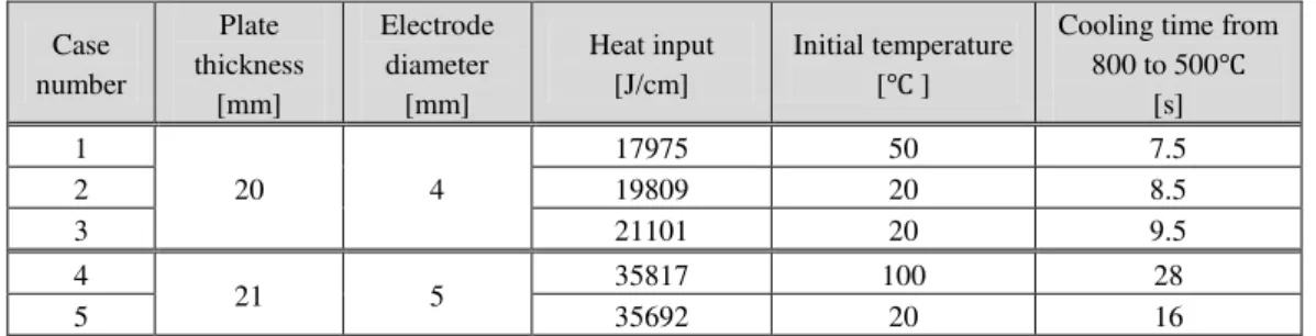
The first series of simulations was performed for the case 1 in Table 2. For the heat input given in Table 2, characteristics of the heat source given in Table 1, and the efficiency of , the velocity of the heat source is which was rounded to in calculations. The parameters of the double ellipsoidal heat source have been chosen randomly in order to carry out some kind of calibration of the heat source. The end time of simulations, , was chosen so that the temperature at the point ( ) m drops below ℃. The results are presented in Figure 2.
The three resulting curves in Figure 2 are marked additionally with symbols to highlight the differences. First is the one marked with stars where the semi-axis of a double ellipsoid is . The resulting maximal temperature is ℃ and is much higher than the measured temperature of ℃. The last two curves have , and other parameters have the same value, which is somewhat higher than in the other calculations, and . The resulting maximal temperature is still much higher but is approaching measured maximal temperature.
Figure 2. Numerical results for the temperature as a function of time for the first series of randomly selected double ellipsoid parameters for the point in the symmetry plane ( 0), at 0 05 and 0 004 , obtained for the case 1 in Table 2
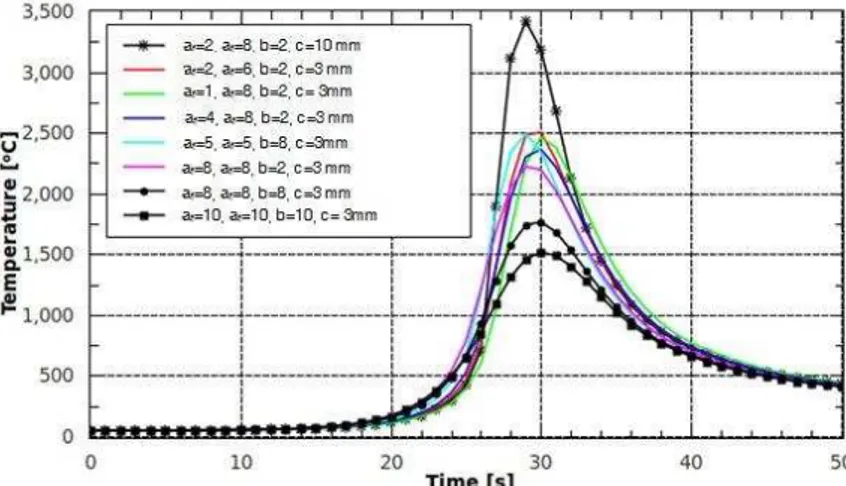
The calibration of the heat source has been continued for a couple more combinations of parameters. The results are illustrated in Figure 3. Again, the two resulting curves are marked additionally with symbols to highlight that the maximal temperature reached at the position ( ) m is slightly lower (blue line), or higher (red line), than the measured temperature. The combination of parameters presented with the blue line that results with the maximal temperature of ℃ was chosen for further calculations that include cases 1-3 from Table 2. At the position , the constant maximal value of the temperature that will be reached on the plate has still not been reached, which is the reason why the combination of parameters that produces the lower value of maximal temperature is selected for further simulations.
maximal temperature at the plate is approximately ℃, and the maximal temperature at the selected point is approximately ℃ (measured temperature is ℃).
Figure 3. Numerical results for the temperature as a function of time for the second series of randomly
selected double ellipsoid parameters for the point in the symmetry plane ( 0), at 0 05 and
0 004 , obtained for the case 1 in Table 2
Figure 4. Temperature distribution presented in cut planes distributed at every 2 in front and
behind the position 0 2 at time 125 when the temperature reaches the maximal value at the
symmetry plane ( 0), at the point 0 2 and 0 004 (marked with a blue dot).
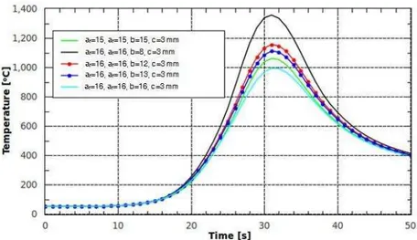
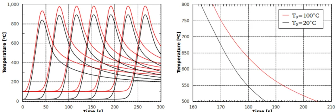
Simulations were continued for cases 2 and 3. For these cases, the initial temperature of the plate was ℃, and velocities of the heat source were rounded to , and respectively. The results are illustrated in Figure 5. Values for the cooling time obtained numerically, for case 1, for case 2, and for case 3, are pretty close to the experimentally measured values, for case 1, for case 2, and for case 3.
The calibration of the heat source was repeated for the last two cases from Table 2
are presented in Figure 6. The last combination of parameters resulted with the maximal temperature of approximately ℃ which is lower than, and closest to, the measured maximal temperature of ℃.
Figure 5. Temperature as a function of time at the position 0 2 0 0 004 for cases 1, 2, and 3
presented in Table 2 (left figure), and cooling time for the same cases (right figure)
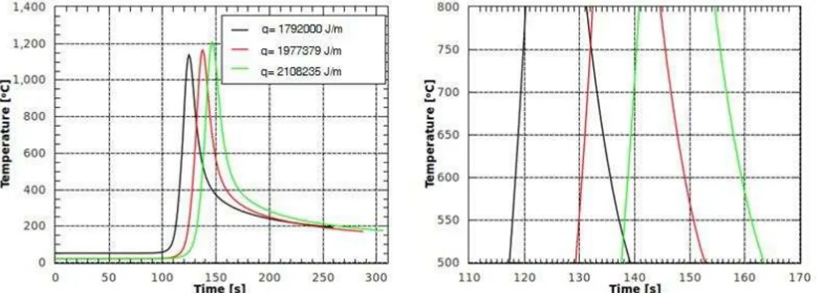
Figure 6. Numerical results for the temperature as a function of time for the series of randomly selected double ellipsoid parameters for the point in the symmetry plane ( 0), at 0 05 and 0 004 , obtained for the case 4 in Table 2
The temperature distribution for the last combination of the heat source parameters applied to the fourth case is illustrated in Figure 7. Temperature distribution for this case was chosen to be presented as the most illustrative. The initial temperature of the plate was the highest, the value of the heat input was higher and the velocity was lower than in the previous cases, and therefore the cooling of the plate was slower.
At ,(Figure 7 left), the maximal value of temperature at point is reached. At that time, the center of the source is more than in front of the point. At , (Figure 7 right), the maximal value of temperature at point is reached and the center of the source is almost in front of the point. The maximal temperature of the plate at is approximately ℃ while the maximal temperature that was reached on the plate is approximately ℃ (Figure 7 right).
The temperature distribution in cut planes around the position is illustrated in Figure 8. The maximal temperature at point is approximately ℃. The temperature is ℃ higher than the measured temperature.
Figure 8. Temperature distribution presented in cut planes distributed at every 10 in front and
behind the position 0 35 at time 267 when the temperature reaches the maximal value at the
symmetry plane ( 0), at the point 0 35 and 0 004 (marked with a blue dot).
Figure 9. Temperature as a function of time at positions 0 05, 0 1, 0 15, 0 2, 0 25, 0 3, and 0.35 m
0 0 004 for cases 4-5 presented in Table 2 (left), and cooling time for the same cases (right)
Conclusion
The selected series of experimental results was divided into two groups. A criterion was the characteristic of the heat source or, more precisely, the characteristic of the electrode. An available input data was the heat input, and an available output data was the maximal value of temperature at only one point in the heat effected zone and the cooling time from ℃ to ℃ for that point. Numerous calculations have been executed in an attempt to set the parameters of the numerical heat source. The double ellipsoidal heat source is complex, the possibilities are numerous, but the question still stands – how to decide which the correct principle of selection of parameters is.
References
[1] M. Berkovic, S. Maksimovic and A. Sedmak, "Analysis of Welded Joints by Applying the Finite Element Method," Structural Integrity and Life, 4 (2004), 2, pp. 75-83.
[2] V. N. Lazic, A. S. Sedmak, M. M. Zivkovic, S. M. Aleksandrovic, R. D. Cukic, R. D. Jovicic and I. B. Ivanovic, "Determining Of Cooling Time (t8/5) In Hard Facing Of Steels For Forging Dies," Thermal
science, 14 (2010), 1, pp. 235-246.
[3] S. Cvetkovski, L. P. Karjalainen, V. Kujanpaa and A. Ahmad, "Welding Heat Input Determination In TIG And Laser Welding of Ldx 2101 Steel by Implementing The Adams Equation For 2-D Heat Distribution," Structural Integrity and Life, 10 (2010), 2, pp. 103-109.
[4] D. Kalaba, A. Sedmak, Z. Radakovic and M. Miloš, "Thermomechanical Modeling the Resistance Welding of Pbsb Alloy" Thermal Science, 14 (2010), 2, pp. 437-450.
[5] W. Perret, C. Schwenk and M. Rethmeier, "Comparison of analytical and numerical welding temperature field calculation," Computational Materials Science, 47 (2010), 4, pp. 1005-1015.
[6] J. Goldak, A. Chakravarti and M. Bibby, "A New Finite Element Model for Welding Heat Sources,"
Metallurgical transactions B, 15 (1984), 2, pp. 299-305.
[7] M.C. Smith and A.C. Smith, "NeT bead-on-plate round robin: Comparison of transient thermal predictions and measurements," International Journal of Pressure Vessels and Piping, 86 (2009), 1, pp. 96-109.
[8] A. Pahkamaa, L. Karlsson, J. Pavasson, M. Karlberg, M. Nasstrom and J. Goldak, "A Method To Improve Efficiency In Welding Simulations For Simulation Driven Design," in ASME 2010 International Design Engineering Technical Conference & Computers and Information in Engineering Conference IDETC/CIE 2010, Montreal, Quebec, Canada, 2010.
[9]
[10]
[11]
J. Goldak, M. Asadi and R. Garcia Alena, "Why power per unit length of weld does not characterize a weld" Computational Materials Science, 48 (2010),2, pp. 390-401.
Veljic, M. Perovic, A. Sedmak, M. Rakin, N. Bajić, B. Medjo, H. Dascau, Numerical Simulation of the Plunge Stage in Friction Stir Welding, Structural Integrity and Life, 11 (2011), 2, pp.131-134.
I.Atanasovska, D.Momčilović, M.Burzić, T.Vuherer, Coupled Nonlineary Problems in Finite Element Analysis – A Case Study, Structural Integrity and Life, 12 (2012), 3, pp.201-208.
[12] V. N. Lazic, Optimization of surface welding process from the point of view of tribological characteristics of surface layer and residual stress (in Serbian), Ph.D. Thesis, Faculty of Mechanical Engineering, University of Kragujevac, Serbia, 2000.
[13] Code Aster, "Documentation version 11" [Online]. Available: www.code-aster.org. ]