www.biogeosciences.net/6/2265/2009/
© Author(s) 2009. This work is distributed under the Creative Commons Attribution 3.0 License.
Biogeosciences
Modelling regional scale surface fluxes, meteorology and CO
2
mixing ratios for the Cabauw tower in the Netherlands
L. F. Tolk1, W. Peters2, A. G. C. A. Meesters1, M. Groenendijk1, A. T. Vermeulen3, G. J. Steeneveld2, and A. J. Dolman1
1VU University Amsterdam, Amsterdam, The Netherlands
2Wageningen University and Research Centre, Wageningen, The Netherlands 3Energy Research Centre of the Netherlands, Petten, The Netherlands
Received: 2 May 2009 – Published in Biogeosciences Discuss.: 22 June 2009
Revised: 30 September 2009 – Accepted: 9 October 2009 – Published: 26 October 2009
Abstract. We simulated meteorology and atmospheric CO2 transport over the Netherlands with the mesoscale
model RAMS-Leaf3 coupled to the biospheric CO2 flux
model 5PM. The results were compared with meteorologi-cal and CO2 observations, with emphasis on the tall tower
of Cabauw. An analysis of the coupled exchange of en-ergy, moisture and CO2 showed that the surface fluxes in
the domain strongly influenced the atmospheric properties. The majority of the variability in the afternoon CO2mixing
ratio in the middle of the domain was determined by bio-spheric and fossil fuel CO2fluxes in the limited area domain
(640×640 km). Variation of the surface CO2fluxes,
reflect-ing the uncertainty of the parameters in the CO2flux model
5PM, resulted in a range of simulated atmospheric CO2
mix-ing ratios of on average 11.7 ppm in the well-mixed boundary layer. Additionally, we found that observed surface energy fluxes and observed atmospheric temperature and moisture could not be reconciled with the simulations. Including this as an uncertainty in the simulation of surface energy fluxes changed simulated atmospheric vertical mixing and horizon-tal advection, leading to differences in simulated CO2of on
average 1.7 ppm. This is an important source of uncertainty and should be accounted for to avoid biased calculations of the CO2mixing ratio, but it does not overwhelm the signal
in the CO2mixing ratio due to the uncertainty range of the
surface CO2fluxes.
Correspondence to:L. F. Tolk ([email protected])
1 Introduction
Terrestrial carbon uptake is an important process in the global carbon cycle. It removes a substantial part of the an-thropogenic emitted CO2from the atmosphere (Canadell et
al., 2007). A useful method to increase our understanding of the terrestrial CO2fluxes is inverse modelling of atmospheric
CO2mixing ratio observations (e.g. Gurney et al., 2002). In
this method the atmospheric signal is used to constrain the surface fluxes using an atmospheric transport model. The re-sults of inversion calculations depend to a large extent on the quality of atmospheric modelling (Stephens et al., 2007).
Therefore, correct simulation of the atmospheric transport, and accounting for the uncertainties, is an important goal in inverse modelling of CO2. Atmospheric transport is
mod-elled at increasingly higher resolutions to capture the high spatial and temporal variability in observed CO2mixing
ra-tios over the continent. Continental scale studies show that the forward simulation of CO2improved by increasing the
horizontal resolution from a number of degrees (Gurney et al., 2002) to one degree or less (Geels et al., 2007; Parazoo et al., 2008). Further increasing the horizontal resolution to just a few kilometres in more limited domain studies (Dolman et al., 2006) was shown to improve the CO2 mixing ratio
simulation at observation stations in uneven and coastal ter-rain, because of the models ability to simulate mesoscale circulations, like sea breezes and topography induced kata-batic flows (Nicholls et al., 2004; Riley et al., 2005; Van der Molen and Dolman, 2007; Sarrat et al., 2007; Ahmadov et al., 2009). This also avoids representation errors by resolv-ing a larger part of the variability in the CO2 mixing ratio
Despite these achievements correct modelling of the CO2
mixing ratios remains challenging. Model intercomparisons of global (Stephens et al., 2007; Law et al., 2008), continen-tal (Geels et al., 2007) and mesoscale models (Van Lipzig et al., 2006; Sarrat et al., 2007) showed discrepancies in the meteorology and CO2modelled of different models. In the
simulation of CO2mixing ratios both advection and
entrain-ment play an important role (Vila et al., 2004; Casso-Torralba et al., 2008) and the quantification of uncertainties in these physical processes is one of the major questions in transport modelling. Comparisons at a coarser scale with observa-tions showed that an erroneous simulation of the advection (Lin and Gerbig, 2005) and of vertical mixing (Gerbig et al., 2008) can lead to uncertainties in the simulated CO2
mix-ing ratio of several ppm. Here we study at regional scale the effect of surface flux uncertainties on these transport errors.
In the present study a high resolution simulation is performed with the non-hydrostatic Regional Atmospheric Modeling System (RAMS; Pielke et al., 1992). The per-formance of the simulation is assessed with meteorological and CO2observations. We address a potential source of
er-ror in the simulated atmospheric vertical mixing: the simula-tion of the surface energy fluxes. Its uncertainty is estimated based on a comparison of different models (RAMS, WRF and ECMWF) and by using different parameter values in the surface flux model within RAMS. The model simulations are compared with both surface flux observations and with atmo-spheric CO2mixing ratio observations.
We coupled the biospheric CO2 flux model 5PM to the
RAMS atmospheric transport model, in order to study the coupled exchange of energy, moisture and CO2. In this
framework the impact of the surface energy fluxes on the simulation of atmospheric transport and consequently on the CO2 mixing ratio is quantified. Novel in our approach is
that we distil the impact of the uncertainty in the simulated surface energy fluxes on the atmospheric CO2mixing ratio,
and that we quantify this CO2 transport error in a Eulerian
approach.
Also, the uncertainty in the CO2 surface fluxes is
ad-dressed. With the coupled RAMS-5PM simulation system these are propagated into a range of CO2mixing ratios. This
indicates the minimal performance of the atmospheric trans-port model required for the use in inversion studies, since the uncertainty in the transport modelling should not exceed the uncertainty related to CO2surface flux uncertainty. The
pa-rameters in the biospheric model 5PM have been optimized in a previous study for a number of eddy correlation flux ob-servations (Groenendijk et al., 2009). Innovative in this study is that we show at mesoscale a realistic uncertainty range of CO2 mixing ratios due to uncertainties in the CO2 surface
fluxes, based on independently determined a-priori flux esti-mates.
Finally, we separate the contribution of different CO2
sources and sinks to the CO2mixing ratio at Cabauw, i.e. the
influence of the advection of CO2 into our domain
(back-ground contribution), the fossil fuel emissions, sea-air CO2
exchange, and terrestrial respiration and assimilation fluxes. The relative importance of the different CO2 contributions
indicates which uncertainties in the surface CO2fluxes are
important and which can be neglected. Additionally, the rel-ative contribution of the near field versus the far field fluxes on the CO2mixing ratio is shown, another important subject
in regional scale inverse modelling (Zupanski et al., 2007; Lauvaux et al., 2008; Gerbig et al., 2009).
The paper is organized as follows: in Sect. 2 the simulation set-up is described, in Sect. 3 the performance of the model is validated against meteorological observations, Sect. 4 de-scribes the simulated CO2fluxes and mixing ratios compared
to observations and in Sect. 5 the implications of our results for the interpretation of the observations, future forward and inverse CO2simulations are discussed.
2 Methods
2.1 Simulation period and domain
We performed simulations with the Regional Atmospheric Modeling System (RAMS) for 22 days in June 2006. In this time of year the biogenic assimilation fluxes during daytime of CO2were large. This period was selected because it
cov-ers a number of meteorological regimes with different wind directions and frontal passages, influencing the atmospheric properties and carbon exchange. South-easterly winds coin-cided with clear sky conditions, while northerly and south-westerly winds caused more cloudy conditions.
A two way nested grid was used (Fig. 1) centred on the Netherlands at 52.25◦N and 5.2◦E, with a 320×320 km
do-main at 4 km resolution nested in a 640×640 km domain at 16 km resolution (Table 1). The centre of the domain is rela-tively flat, with a maximum elevation of∼100 m. The
south-east part of the domain has more orography, up to∼500 m.
The dominant land use types in the area are cultivated lands (crops and grasslands) and urban areas. Large cities and in-dustrial areas of the Netherlands, Belgium and the German Ruhr Area are within the domain. To the north and the west the Netherlands is bounded by the North Sea.
2.2 Simulation setup
The atmospheric simulations were performed with the non-hydrostatic mesoscale model RAMS (Pielke et al., 1992), which has already been used to simulate the behaviour of CO2in the atmosphere in a number of studies (e.g. Denning
Longitude
Latitude
2 4 6 8 10
50 51 52 53 54 55
4 5 6 7
51 51.5 52 52.5 53 53.5
Crops Grass Broadleaf forest Needle leaf forest Urban
0510 0 50 100
Cabauw (grass) Sc (grass) EC (forest) EC (grass) EC (crops) Radiosonde
Fig. 1. Simulation domain with 2 nested grids. The star indicates Cabauw, the square the location of the radiosonde release, the triangles indicate the scintillometers and the dots the eddy correlation observations.
their Eq. (9)). This scheme uses a non-local turbulence pa-rameterization within the convective boundary layer. Inclu-sion of this within the medium range forecast (MRF) model has been shown by Troen and Mahrt (1986), Holtslag et al. (1995) and Hong and Pan (1996) to simulate the day-time boundary layer structures more realistically than local mixing schemes. In our simulations with RAMS we applied this non-local scheme also to the CO2-transport. Cumulus
convection was not parameterized in the simulations. The surface energy fluxes were simulated using Leaf-3 (Walko et al., 2000). The vegetation Leaf Area Index (LAI) of the MODIS database was used.
Meteorology, soil temperature and soil moisture were ini-tialized with ECMWF analysis data (Uppala et al., 2005). In order to be consistent with the RAMS soil wilting point (wp) and field capacity (fc), the ECMWF soil moisture (η) was scaled towards RAMS soil variables based on a soil wetness index (SWI):
SWI= η−ηwp
ηf c−ηwp (1)
ηRAMS =ηwp,RAMS+SWI
ECMWF ηf c,RAMS−ηwp,RAMS
(2) Optimized CO2mixing ratio fields at 1×1◦resolution from
CarbonTracker Europe (Peters et al., 2009) were used for ini-tial and boundary conditions of the CO2mixing ratio. The
simulations were nudged every 3 h to CarbonTracker CO2
mixing ratios and every 6 h to the ECMWF analysis mete-orology with a nudging relaxation time scale of 900 s. The nudging extended inward from the lateral boundary by 5 grid cells and the centre of the domain was free of nudging.
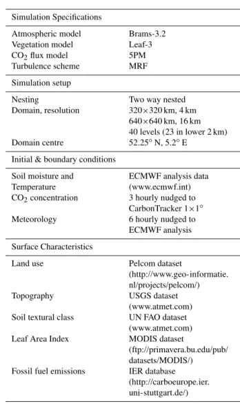
Table 1.Specification of the simulation settings.
Simulation Specifications
Atmospheric model Brams-3.2
Vegetation model Leaf-3
CO2flux model 5PM
Turbulence scheme MRF
Simulation setup
Nesting Two way nested
Domain, resolution 320×320 km, 4 km
640×640 km, 16 km
40 levels (23 in lower 2 km)
Domain centre 52.25◦N, 5.2◦E
Initial & boundary conditions
Soil moisture and Temperature
ECMWF analysis data (www.ecmwf.int)
CO2concentration 3 hourly nudged to
CarbonTracker 1×1◦
Meteorology 6 hourly nudged to
ECMWF analysis
Surface Characteristics
Land use Pelcom dataset
(http://www.geo-informatie. nl/projects/pelcom/)
Topography USGS dataset
(www.atmet.com)
Soil textural class UN FAO dataset
(www.atmet.com)
Leaf Area Index MODIS dataset
(ftp://primavera.bu.edu/pub/ datasets/MODIS/)
Fossil fuel emissions IER database
2.3 CO2fluxes
CO2fluxes from fossil fuel burning were included in the
sim-ulations based on the IER database at 10 km resolution (http: //carboeurope.ier.uni-stuttgart.de/). The CO2fluxes from the
coastal sea inside the domain were calculated based on cli-matologic estimates of the partial pressure of CO2in the sea
(Wanninkhof, 1992; Takahashi et al., 2002). Biospheric CO2
surface fluxes were modelled with 5PM (Groenendijk et al., 2009). This model was coupled to RAMS through the ra-diation, the temperature and humidity of the canopy air and influences the CO2 mixing ratio at the lowest atmospheric
level. The CO2assimilation does in this model not depend
on the energy fluxes of RAMS through the stomatal con-ductance (Collatz et al., 1991) or on Leaf Area Index (LAI) (Sellers et al., 1996). In 5PM the photosynthesis is calcu-lated following Farquhar et al. (1980), where photosynthesis is either limited by the carboxylation rate, which is enzyme limited, or by the light limited RuBP regeneration rate. The most important assimilation parameters in this model are the maximum carboxylation capacity (Vcmax)and the light use
efficiency (α). Respiration was calculated with the relation-ship by Lloyd and Taylor (1994):
R=R10 e
E0 ℜ
1 283.15−T0−
1 T−T0
(3) whereR10is the respiration rate at a reference temperature
of 10◦C, E0
ℜ is the activation energy divided by the universal
gas constant,T0is a constant of 227.13 K andTis soil
tem-perature. For further specifications of 5PM see Groenendijk et al. (2009).
Groenendijk et al. (2009) optimized the parameters of this model (Vcmax, α, R10 and E0) for the full canopy based
on a large number of Fluxnet observations (Baldocchi et al., 2001). We applied parameter values optimized for the temperate zone, for the period of May–July for all years (Table 2). The parameter values used in our simulations were kept constant in time. Simulations were performed with CO2
fluxes calculated based on the best guess parameter values. For respiration and assimilation of the most abundant vegeta-tion species (crops and grass) we also simulated fluxes using the upper and the lower parameter values within the standard deviation of the parameter estimate. In this way a range of CO2mixing ratios was simulated based on the different CO2
flux parameter settings. In the rest of this work, we report the range of uncertainties, i.e. the difference between the highest and lowest values in our set of simulations. Further specifi-cations on the design of the simulations are given in Table 1.
2.4 Observations
A large number of observations of the atmospheric proper-ties and the surface fluxes were available for model valida-tion. Data from continuous CO2mixing ratio measurements,
performed by a Licor 7000 with a precision of 0.05 ppm, and
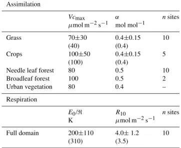
Table 2. CO2 flux parameter settings based on Groenendijk et
al. (2009). Vcmaxis the full canopy maximum carboxylation
ca-pacity, αthe light use efficiency for the full canopy,E0/ℜis the
respiration activation energy divided by the universal gas constant,
R10is the respiration rate at 10◦C and n sites indicates the number
of sites used in the optimizations of the parameters. Where uncer-tainty ranges are shown the best guess, upper and lower estimates of the parameters are used in the simulations. In between brackets
the parameter values that returned the best CO2mixing ratios.
Assimilation
Vcmax
µmol m−2s−1
α
mol mol−1
nsites
Grass 70±30
(40)
0.4±0.15
(0.4)
10
Crops 100±50
(100)
0.4±0.15
(0.4)
5
Needle leaf forest 80 0.5 10
Broadleaf forest 100 0.5 2
Urban vegetation 80 0.4 –
Respiration
E0/ℜ
K
R10
µmol m−2s−1
nsites
Full domain 200±110
(310)
4.0±1.2
(3.5)
10
meteorological data from the tall tower at Cabauw at a height of 20 m, 60 m, 120 m and 200 m were used. Also, atmo-spheric observations for temperature, humidity, wind speed and direction were available at 110 synoptic 2 m stations over the Netherlands and from the radiosondes that were released twice a day at De Bilt, which is about 25 km north-east of the Cabauw site. Observations of the surface fluxes were available for sensible heat, latent heat and CO2fluxes from
eddy correlation measurements (Aubinet et al., 2001; Dol-man et al., 2002; Wilson et al., 2002; Jacobs et al., 2007; Braam, 2008; Aubinet et al., 2009). Additionally, scintil-lometer measurements provided extra sensible heat flux mea-surements over a horizontal path of 0.35–5 km (De Bruin et al., 2004). The locations are specified in Fig. 1 and in Table 3.
3 Results: Meteorological performance of the model
3.1 Consistency of the simulation in time
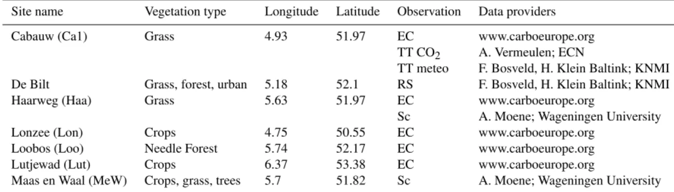
Table 3.Observation specifications. EC is eddy correlation measurements, Sc is scintillometer, RS is radiosonde and TT is tall tower.
Site name Vegetation type Longitude Latitude Observation Data providers
Cabauw (Ca1) Grass 4.93 51.97 EC www.carboeurope.org
TT CO2 A. Vermeulen; ECN
TT meteo F. Bosveld, H. Klein Baltink; KNMI
De Bilt Grass, forest, urban 5.18 52.1 RS F. Bosveld, H. Klein Baltink; KNMI
Haarweg (Haa) Grass 5.63 51.97 EC www.carboeurope.org
Sc A. Moene; Wageningen University
Lonzee (Lon) Crops 4.75 50.55 EC www.carboeurope.org
Loobos (Loo) Needle Forest 5.74 52.17 EC www.carboeurope.org
Lutjewad (Lut) Crops 6.37 53.38 EC www.carboeurope.org
Maas en Waal (MeW) Crops, grass, trees 5.7 51.82 Sc A. Moene; Wageningen University
south-westerly winds brought more cloudy conditions with reduced radiation, lower temperatures and smaller nocturnal cooling.
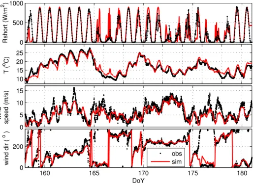
Here we show the results of the standard simulation used in this study. For this simulation, the standard RAMS set-tings have been modified to obtain a more realistic Bowen ra-tio, as will be described in Sect. 3.2. The model reproduced the synoptic variations over the full 22-day period without any re-initialization of the simulation (Fig. 2 and Table 4). This was achieved by prescribing boundary conditions from reanalysis products such as ECMWF meteorology and Car-bonTracker CO2mixing ratios. A change in the large-scale
atmospheric situation was thus passed on to the inner do-main for which RAMS simulated, mimicking the effect of a initialization. A large advantage of not needing to re-initialize the RAMS model over multi-week periods is that mass continuity of tracers and a balance of the physical equa-tions for energy and water was ensured.
A comparison of the statistics for the first and last half of the period showed the consistency of the model performance in time (Table 4). Hourly temperature (T) and humidity (q) were simulated comparably well in both periods. Radiation showed a better performance in the first half of the period, which can be attributed to the occurrence of clouds in the second half of the period, rather than to a drift of the simu-lated meteorology with time. Incoming solar radiation and its reduction by clouds was mostly simulated with the cor-rect amplitude and frequency. However, the exact location of the clouds and subsequently the timing of the radiation reduction sometimes deviated from the observations, as was also seen in similar mesoscale model studies (Denning et al., 2003; Van Lipzig et al., 2006; Parazoo et al., 2008).
3.2 Uncertainties in the surface energy fluxes
Surface energy fluxes are important drivers of processes in the atmosphere, influencing amongst others the atmospheric
T,qand vertical mixing. Uncertainties in the surface energy fluxes thus may be an important source of uncertainty in the
simulation of the atmospheric properties and are addressed in this section.
We compared the simulated energy fluxes with eddy co-variance and scintillometer measurements (Fig. 3) and made a comparison with two other models: WRF and ECMWF. Additionally, we studied the sensitivity of the simulated sen-sible (H) and latent (LE) heat fluxes to changes in the surface flux calculation by Leaf3, and its effect on the atmosphere. This revealed that the simulations at some days either cap-tured the observed surface energy fluxes, or the observedT
andqvertical profile in the planetary boundary layer (PBL), but could not reconcile both. The atmospheric observations and the comparison with other models suggested a higher Bowen ratio (i.e. the ratio of sensible to latent heat flux,β) than simulated with standard Leaf3 settings. Possible options for such an increasedβ are shown in Table 5 and described below, with a focus onTandHbecause of their importance for atmospheric vertical mixing.
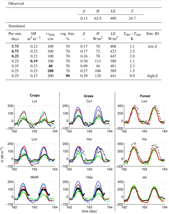
The energy fluxes showed a large variation between low (crops, grasslands) and high (forest) vegetation types (Fig. 3, note the different scale on the y-axis for low and high vegeta-tion). These differences were driven by differing vegetation characteristics such as the low aerodynamic resistance and stomatal conductance in forest and were reproduced in the RAMS simulations.
With the standard Leaf3 vegetation characteristics (green line in Fig. 3) most of the eddy correlation observations were captured reasonably well. The scintillometer observa-tions at Maas-en-Waal and Haarweg were slightly underes-timated. With these settings the PBLT was underestimated andqoverestimated at clear days with eastern winds, in com-parison with radiosonde observations (Fig. 4 and Table 5), the Cabauw tall tower and synoptic 2 m observations (not shown).
160 165 170 175 180 0
500 1000
Rshort (W/m
2 )
160 162 164 166 168 170 172 174 176 178 180
10 15 20 25
T (
o C)
160 165 170 175 180
0 5 10 15
wind
speed (m/s)
160 165 170 175 180
0 200
wind dir (
o )
DoY
obs sim
Fig. 2.Observed and simulated time series at the Cabauw of(a)short wave radiation,(b)potential temperature,(c)wind speed and(d)wind direction at 200 m.
Table 4.Statistics of the simulation, in comparison with observations of the potential temperature (T) and CO2at 20 m and 200 m, humidity
(q) at 2 m and the incoming shortwave radiation (rshort) at Cabauw, for the full period, the first and the second half of the simulation period.
Humidity is compared to the simulated canopy air humidity, CO2andTwith simulated atmospheric values.
Full period First half Second half
R2 RMSE R2 RMSE R2 RMSE
T 200 m 0.90 1.2 K 0.92 1.2 K 0.87 1.1 K
T 20 m 0.87 1.4 K 0.92 1.3 K 0.80 1.5 K
q 2 m 0.51 1.1 g kg−1 0.47 1.3 g kg−1 0.65 0.8 g kg−1
Rshort 0.78 143.4 W m−2 0.88 113.2 W m−2 0.64 165.6 W m−2
CO2200 m 0.21 5.9 ppm 0.15 5.8 ppm 0.23 6.3 ppm
CO220 m 0.67 10.1 ppm 0.71 11.0 ppm 0.55 9.8 ppm
matched the observedT well (not shown), but also failed to match the observedHfor grass and crops (light and dark blue lines in Fig. 3).
Sensitivity tests showed that the strength ofLEandH de-pended strongly on (1) the water availability, (2) the minimal stomatal resistance, which determines the plants’ resistance to transport of water and CO2and (3) the fraction of the
sur-face that is vegetated (Table 5).
(1) Decreasing the soil moisture content led to a strong increase inβ, because of the decrease in evaporation from the soil and transpiration from the plants. (2) Also a dou-bling of the minimal stomatal resistance, a rather uncertain
parameter in Leaf3 (Walko et al., 2000), for grass and crops from 100 sm−1to 200 sm−1increasedβ. (3) With standard Leaf3 settings the vegetation fraction of grass and crops did not exceed∼70%, even with a high LAI. We increased the
vegetation fraction to 90% when the LAI is larger than 1, in line with for example the settings in the ECMWF surface model. This increase led to a considerable increase inHand the atmosphericT(Table 5).
Table 5.Overview of the sensitivity tests. Results are given for 11 June 12:00. Simulation settings: Pre-sim is the time simulated before this
moment,SMis the soil moisture content,rsminis the minimal stomatal resistance of the low vegetation, veg. frac. is the vegetation fraction.
Results: Bowen ratio (β), sensible (H) and latent (LE) heat flux, all for Cabauw; and observed potential temperature (T) for De Bilt at 500 m
height (radiosonde observation), and its difference (Tsim−Tobs) with the simulated value. Sim. ID identifies the two simulations further used
in this study (for more information see the text). The bold numbers indicate the change compared to the preceding simulation.
Observed
β H LE T
0.13 62.9 480 24.7
Simulated
Pre-sim. SM rsmin veg. frac. β H LE Tobs−Tsim Sim. ID
days m3m−3 s/m % – W/m2 W/m2 K
5.75 0.23 100 70 0.17 70 408 3.1 lowβ
0.75 0.23 100 70 0.17 72 423 2.5
0.25 0.23 100 70 0.16 70 447 2.0
0.25 0.19 100 70 0.30 113 380 1.1
0.25 0.23 40 70 0.09 44 481 2.3
0.25 0.23 200 70 0.27 106 389 1.5
0.25 0.23 200 90 0.29 128 441 0.9 highβ
162 163 164
−100 0 100 200
Ca1
162 163 164
−200 0 200 400
Loo
162 163 164
−100 0 100 200
Lut
162 163 164
−100 0 100 200
Haa
time (doy)
162 163 164
−100 0 100 200
Hor
162 163 164
−200 0 200 400
Vie
162 163 164
−100 0 100 200
Lon
H (W m
−2 )
162 163 164
−200 0 200 400
Jal
162 163 164
−100 0 100 200
MeW
Crops Grass Forest
15 20 25 30 35 0
1000 2000 3000
Theta (oC)
Height (m)
12:00
15 20 25 30 35
0 1000 2000 3000
Theta (oC) 24:00
0 5 10
0 1000 2000 3000
q (g/kg)
Height (m)
0 5 10
0 1000 2000 3000
q (g/kg)
370 380 390
0 1000 2000 3000
Height (m)
CO2 mixing ratio (ppm)
370 380 390
0 1000 2000 3000
CO2 mixing ratio (ppm) c.
b. a.
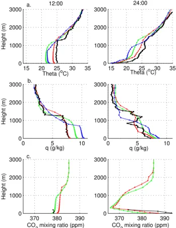
Fig. 4. Simulated and observed potential temperature(a)and
hu-midity(b)profiles at De Bilt, and CO2mixing ratio(c)profiles at
Cabauw, 11 June 2006, at 12:00 (left) and 24:00 (right). Black in-dicates the radiosonde (a), (b) or tall tower (c) observations, red the simulation with a high Bowen ratio, green the simulation with a low Bowen ratio. Blue indicates the simulated temperature and humid-ity with a low Bowen ratio, but with the Mellor Yamada instead of MRF turbulence scheme.
We will refer to the simulation with increased stomatal re-sistance and vegetation fraction and standard soil moisture as the “highβ simulation”, while the simulation with stan-dard Leaf3 vegetation characteristics will be referred to as the “lowβsimulation”.
These two cases however do not capture the full range of uncertainty in beta, as even the low beta simulation some-times still overestimatesHand underestimatesLE(Fig. 3 and Table 5). Decreasing for example the stomatal resistance as suggested for Cabauw by Jackson et al. (2003) would fur-ther reduceβin such situations (Table 5). The uncertainty in surface energy fluxes may thus even be larger than inferred here from the atmospheric observations, indicating that our uncertainty estimates may be conservative.
We tested the sensitivity of our findings to the moment of initialization. When initialized 6 h, 18 h or over 5 days in
advance, the simulated noon temperatures deviated 2.0, 2.5 or 3.1 K from the observations, respectively (Table 5) using the settings yielding the lowβ. Hence, the largest part of the temperature underestimation built up within a few hours and was rather independent of the moment of initialization. For the highβ simulation the results were robust to a change of the moment of initialization (not shown).
The fact that the surface flux observations and the atmo-spheric observations both suggest different optimalβ’s indi-cated an uncertainty in what the correctβ should be in the simulations for the full domain. Further discussion on this will be presented in Sect. 5. We will use the simulation with the highβ(and hence lowestTandqbias in the atmosphere) to investigate the structure of the simulated CO2fields. This
simulation corresponds to the standard run that was discussed in Sect. 3.1. In the next section the effects of the uncertainty in the surface energy fluxes on the atmospheric vertical mix-ing are addressed.
3.3 Atmospheric temperature and humidity profiles
The results of the simulations with (1) lowβ and (2) highβ were compared with the radiosonde observations in De Bilt (e.g. Fig. 4). Generally a well-mixed PBL developed that has a lower potential temperature and is moister than the free troposphere. At clear nights cooling near the surface led to a shallow (200 m) and stable PBL.
Simulations with the MRF turbulence scheme showed a better performance than the standard RAMS Mellor Yamada turbulence scheme (Fig. 4). Still, the height of the PBL was not always captured correctly and the jump ofT andqwas less pronounced than observed. Increasing the vertical reso-lution to 60 instead of 25 vertical layers in the lower 3 km of the atmosphere did not change this. This may be due to the limited horizontal resolution of 4 km, or to uncertain-ties in the parameterization of vertical transport, like lack of subsidence, too much entrainment or an incorrect free tro-pospheric lapse rate ofT orq. The free tropospheric values are generally assumed reasonable due to the use of ECMWF analysis boundary conditions.
Simulation of the nocturnal PBL is even more challeng-ing. The atmospheric stability during clear nights was sys-tematically underestimated by the model, which is a com-mon feature for most atmospheric transport models (Geels et al., 2007; Gerbig et al., 2008). In the simulation the noc-turnal surface signal reached up to∼400 m while in the
ob-servations it was limited to∼200 m. The poorly simulated
height of the PBL will cause discrepancies in the mixing ra-tios which are not directly related to the magnitude of the CO2fluxes.
160 165 170 175 180 0
5 10
Ca1
160 165 170 175 180
0 5 10
Hor
resp. umol/m
2/s
0 5 10
Lut
160 165 170 175 180
0 5 10
Lon
DoY
160 165 170 175 180
−60 −40 −20 0
Ca1
160 165 170 175 180
−60 −40 −20 0
Hor
Assimilation umol/m
2/s
160 165 170 175 180
−60 −40 −20 0
Lut
160 165 170 175 180
−60 −40 −20 0
Lon
DoY
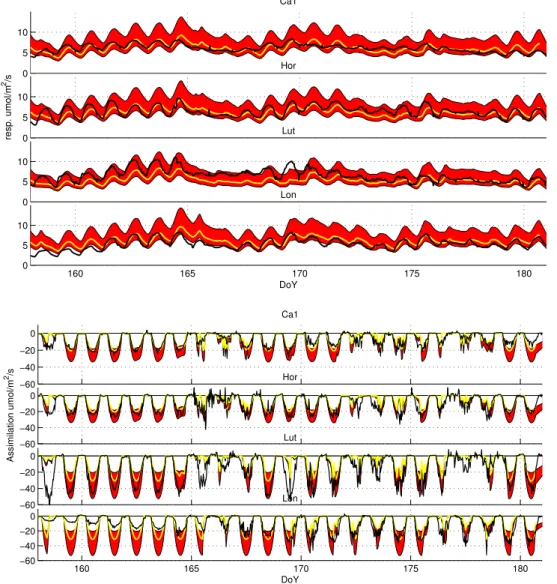
Fig. 5.CO2respiration(a)and assimilation(b)fluxes for 2 grass (Ca1 and Hor) and 2 crops (Lut and Lon) sites. In black the observations.
The red band is the range of CO2fluxes simulated with a spread of biosphere model parameters (Table 2). Yellow shows the simulation that
best fits the CO2mixing ratio observations.
both simulations∼350 m. The simulation with a relative low
β(1, green line in Fig. 4) showed a mean bias of∼−100 m,
while the simulation with a higherβ (2, red line in Fig. 4) had a positive mean bias of∼75 m. The uncertainty in the
surface fluxes can thus explain part of the uncertainty in the simulated PBL height as for example indicated for ECMWF simulations in Gerbig et al. (2008).
4 Results: CO2fluxes and mixing ratios
The framework of the simulated meteorology as described in the previous sections allows us to study the coupling be-tween the surface CO2fluxes and the atmospheric CO2
mix-ing ratios. First, we will address the uncertainties in the CO2
fluxes. Secondly, we will show how these propagate into a range of simulated CO2mixing ratios which is compared to
the observations at the Cabauw tall tower. Finally, the contri-bution of the different CO2fluxes and the background CO2
to the total CO2mixing ratio is unravelled. 4.1 CO2flux variability
The parameters optimized in the biosphere model 5PM showed a rather large variability in time and space, which is reflected in the uncertainty in the average CO2flux parameter
values (Table 2). The range of CO2fluxes (Fig. 5) simulated
with these parameter settings, which were optimized based on European observations for the temperate zone, agreed well with observations and literature values (Jacobs et al., 2007) for our much smaller domain.
CO2fluxes simulated with the parameters that gave an
un-biased result compared to the observed CO2mixing ratio at
160 162 164 166 168 170 172 174 176 178 180 350
400 450 500
20 m
160 162 164 166 168 170 172 174 176 178 180
350 400 450 500
60 m
160 162 164 166 168 170 172 174 176 178 180
350 400 450 500
120 m
160 162 164 166 168 170 172 174 176 178 180
350 400 450 500
200 m
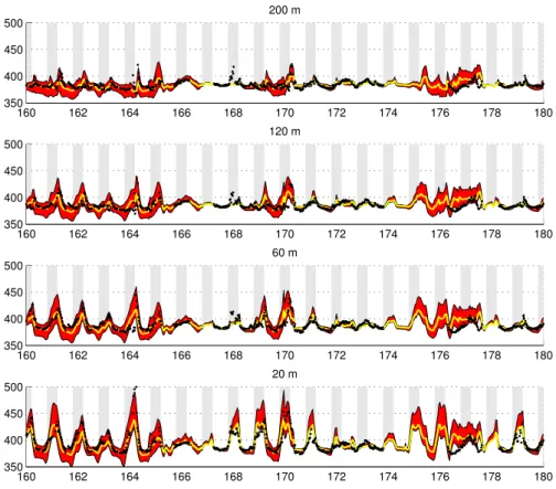
Fig. 6.CO2concentration at 4 heights at Cabauw tower. In black the observations. The red band is the range of CO2mixing ratio simulated
with a spread of CO2flux parameters (Table 2), it reflects the effect of uncertainties in the surface CO2fluxes on the CO2mixing ratios.
brackets in Table 2. Note that in a follow-up study we intend to formally estimate the parameters of the 5PM model based on the forward results presented here, rather than simply se-lecting an unbiased set of values.
Respiration fluxes show a soil temperature driven diur-nal and synoptic variation, which is represented by the model (Fig. 5a). Additionally, the observed respiration fluxes showed differences between sites in magnitude and diurnal amplitude, not observed inT and not included in the model. These kind of variations are meant to be implicitly included in the parameter uncertainties. The observed respiration at Cabauw, Horstermeer and Lonzee are in the lower part of the uncertainty range, while the observations at Lutjewad are often near the top of the range.
Assimilation fluxes were inhomogeneous in space and time as well (Fig. 5b). Generally, the uptake by crops was higher than by grass, as was correctly simulated. Also the observed assimilation reduction at days with limited radia-tion was captured by the model (within the limitaradia-tions of the RAMS radiation calculations). Observed assimilation at Lut-jewad is relatively high and near the maximum of the uncer-tainty range, while Lonzee and Cabauw are near the mini-mum and Horstermeer is in the middle of the range.
Both simulated respiration and assimilation at Lonzee were in the beginning of the period outside the uncertainty range from observations, most likely because the CO2 flux
calculations were not LAI dependent. To overcome this the biosphere model should be extended with spatially explicit, time-varying LAI (e.g. Sellers et al., 1996), which should also give a better representation of the spatial variability of the assimilation fluxes.
Our uncertainty estimates agreed with variability in Dutch grass sites estimated by Jacobs et al. (2007). The standard de-viations of their respiration parameters were almost the same as in our study. Their photosynthesis model, and therefore these parameters are different, but the range is also compa-rable to the range used in this study, with 20–60% variations on the parameters in the GPP model. They concluded that within small regions with relatively uniform climatic condi-tions the variability may be similar to the one observed at European larger scales, as is applied here.
4.2 CO2mixing ratios
Uncertainties in the CO2respiration and assimilation fluxes
had a significant influence on the CO2 mixing ratio when
the air had passed land areas. The different CO2 flux
pa-rameter settings returned a range of simulated CO2mixing
158 160 162 164 166 168 170 172 174 176 178 180 −30
−20 −10 0 10 20 30 40 50
158 160 162 164 166 168 170 172 174 176 178 180
370 380 390
Background
Fossil Fuel Resp. Assim. Grass Asim. Crops Needleleaf Forest Broadleaf forest
Fig. 7.Contribution of the background CO2to the mixing ratio at Cabauw 200 m(a)and the cumulative contribution of the CO2fluxes in
the domain(b). The variation in the CO2mixing ratio is mainly determined by the fossil fuel, respiration and assimilation fluxes, where
atmospheric signal from assimilation by crops dominates over grass assimilation.
when the air predominantly originated from over sea and the land signal is suppressed, while a broader range occurred when the continental signal was large, i.e. with south-easterly wind, low wind speeds or frontal passages. This broad range indicates that the atmospheric mixing ratio potentially con-tains much information about the CO2fluxes within the
sim-ulation domain. This agrees with studies from Lauvaux et al. (2008) and Zupanski et al. (2007) and shows the potential for future inversion on this temporal and spatial scale.
As mentioned previously, the uncertainties in the simula-tion of the meteorology discussed in Sect. 3 give rise to un-certainties in the simulated CO2transport. Here we give an
overview of the impact of those features on the simulation of the CO2mixing ratios.
The uncertainty in the surface energy fluxes (Sect. 3.2) and consequently the vertical mixing (Sect. 3.3) results in an un-certainty in the CO2mixing ratio. To quantify this the results
of the simulations with relative low (1) and high (2) simu-latedβ, were compared for CO2(Fig. 7). These two
simu-lations (with the same CO2flux parameter settings) returned
a difference in the afternoon CO2mixing ratio of on average
1.9 ppm.
This was to a small extent due to changes in the CO2 fluxes between the two simulations. The RMSE of
the total flux change was 0.69µmol m−2s−1. Changes
in the respiration caused by the temperature difference (RMSE=0.63µmol m−2s−1)were systematic. Assimilation fluxes slightly changed due to changes in cloud cover forma-tion (RMSE=0.29µmol m−2s−1), and their difference over the full period was near to zero. Hence, the effect of respi-ration change on the CO2 mixing ratio was relatively large
compared to the assimilation change. Compensating for this
by adjusting theR10left a difference of 1.7 ppm. This
uncer-tainty in the CO2mixing ratio is caused by the difference in
vertical mixing and horizontal advection, due to the surface flux uncertainty.
Other difficulties were related to the simulation of the noc-turnal CO2 mixing ratio, which is up to now, because of
the known large uncertainties in the transport model vertical mixing schemes in stable conditions, not used in inversion studies (Gurney et al., 2002; Stephens et al., 2007; Geels et al., 2007). Our simulations confirm that the simulation of nocturnal CO2is biased, because of the simulation of a too
deep nocturnal PBL (see Sect. 3.3). The absolute nocturnal CO2mixing ratio accumulation was not simulated correctly,
leading to a lowR2 of the CO2mixing ratio time series at
200 m (Table 4) and simulated mixing ratios at 60–200 m that were during some nights totally outside the range of simu-lated CO2mixing ratios. As such it is clear that the
represen-tation of the nocturnal boundary layer in mesoscale models requires improvement.
Nevertheless a significant part of the diurnal variation, es-pecially at lower sample levels, is captured by simulations. During the nights CO2accumulates near the surface and
FF (4.3)
Sea (0.1)
Resp (7.8)
Assim (10.5) Grass (3.5)
Crops (5.3) Nlf (0.4) Blf (0.7) urban (0.1)
Bio FF Sea BG 0
5 10 15
var (ppm
2)
a. b. c.
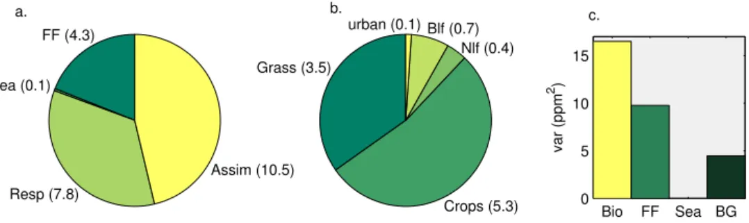
Fig. 8.Average contribution of the different tracers to the diurnal CO2mixing ratio(a)and(b)and its variance(c)at 200 m at Cabauw. (a)
shows the influence of the assimilation (assim), respiration (resp), sea and fossil fuel (FF) fluxes. In (b) the assimilation flux influence is separated by vegetation type: urban vegetation, broadleaf forest (Blf), needle leaf forest (Nlf), crops and grass. In (c) the variability is shown which is due to variations in the biospheric (bio), fossil fuel (FF), and sea fluxes, and in the background mixing ratio (BG).
uncertainty is the simulated location and the timing of the cloud cover (Sect. 3.1). At partly clouded days, this led to an error in simulation of the CO2 fluxes and the depth of
the PBL, and consequently biases in the CO2 mixing ratio.
Therefore, the exact simulated mixing ratios at these days should be regarded as more uncertain. Frontal passages may cause a comparable misrepresentation of the simulated con-centrations (e.g. at 25 June; doy 176).
4.3 Different tracer signals at Cabauw
To study the relative importance of the different sources and sinks influencing the CO2 mixing ratios we separated the
simulated CO2 mixing ratios at Cabauw into contributions
from (a) background CO2entering through the lateral
bound-aries and (b) fluxes from within the RAMS domain. The latter were further separated into contributions from assim-ilation and respiration of different vegetation types, sea-air fluxes and fossil fuel emissions, which were included in the simulation as separate atmospheric tracers (Figs. 7 and 8).
Assimilation and respiration fluxes were important in de-termining the CO2mixing ratio. They had an average
influ-ence during the day of−10.5 and 7.8 ppm respectively, with
peaks up to∼30 ppm at 200 m (Figs. 7 and 8a). In the noctur-nal PBL the respiration tracer showed peaks up to∼60 ppm at 20 m (not shown). The total biosphere signal, i.e. the sum of the respiration and assimilation, was because of the can-celling opposite signs more modest and had an average influ-ence of 3.2 ppm.
Generally, the crops tracer was the most abundant as-similation tracer, even though Cabauw is a grassland site (Fig. 8b). This was due to the relatively high assimilation of crops compared to grass (Fig. 5b) combined with the large area of crops in the domain (Fig. 1).
In our domain the fossil fuel was also an important con-tributor to the total signal. Plumes with high fossil fuel tracer concentrations originating from the industrial sources moved over the domain. The major sources were the Ruhr Area, southeast of the Netherlands, the ports in the southwest of
the Netherlands and in Belgium, and smaller diffuse sources found over the total domain. Afternoon values in the well mixed PBL varied between 2–8 ppm and the average mixing ratio of the fossil fuel fluxes was almost as large as the bio-spheric signal whereas its afternoon variance is half that of the biospheric signal (Fig. 8c).
The contribution of the sea-air CO2 fluxes to the total
signal was very limited at these time scales (Fig. 8a and c), although on a global scale the exchange of CO2 by
the oceans plays an important role. The average flux of
∼0.02µmol m−2s−1at the North Sea was a negligible com-pared to the continental fluxes in the domain.
CO2mixing ratios entering the domain through the lateral
boundaries showed a strong diurnal cycle over land, and a much smaller cycle over the sea. When the wind direction was from the east or south the low daily continental values in the background mixing ratio, caused by assimilation over the continent outside of our simulation domain, reached Cabauw. This was for example seen at 12 and 13 June (doy 163 and 164) when the background concentration was reduced by
∼10 ppm. Because the influence on the mixing ratios in the
middle of the domain can be considerable, the quality of the boundary conditions in a limited domain simulation is im-portant.
5 Discussion and conclusions
We simulated three weeks in June 2006 with the B-RAMS-3.2 mesoscale model at 4 km resolution. The simulations were able to reproduce the observed time series of the me-teorological variables and CO2 mixing ratios satisfactorily
in our simulations a re-initialization of the meteorology was not necessary. The advection of the ECMWF meteorological and CarbonTracker CO2 mixing ratio boundary conditions
over the domain prevents a runaway of the results in a dy-namical and continuous way. This opens the way towards seasonal inversions at a high resolution.
The simulations with the RAMS MRF scheme showed a better performance than the standard Mellor Yamada scheme. This is in line with the findings of Holtslag et al. (1995) and confirms the importance of the parameteriza-tions of turbulence and entrainment (Vila et al., 2004; Casso-Torralba et al., 2008) for the simulation of the atmospheric profiles.
Also a realistic simulation of surface energy fluxes is im-portant for the simulation of atmospheric transport. Compar-ison with other models (WRF, ECMWF) and observations revealed a discrepancy between the simulations and the sur-face observations on the one hand and the atmospheric obser-vations on the other hand. For a number of days the observed
Tprofile could not be reconciled withHobservations, some-thing also seen in previous studies (e.g. Holtslag et al., 1995; Ek and Holtslag, 2004). At those times, the observed PBL height could also not be reproduced with a simple mixed layer model (Vila and Casso-Torralba, 2007) based on the observedH.
The atmospheric observations suggests that the total Bowen ratio (β) over the full domain may be higher than in-dicated by the surface observations. This may be due to het-erogeneity of the energy fluxes within one vegetation type (e.g. Baldocchi et al., 2001) which is not included in our land surface scheme. Also, the limited amount of observa-tions over grass and crops, especially in the eastern part of the domain, and energy balance closure problems (Wilson et al., 2002) of ∼30% for the Cabauw surface flux
obser-vations (Braam, 2008) may add uncertainty to the total sur-face energy flux estimate over the domain. Moreover, (free-standing) houses, trees and roads may lead to a different do-main averagedβthan observed with the surface observations over vegetated terrain only. Hence, optimizations for a single site (e.g. Jackson et al., 2003) may lead to another estimate of the surface energy fluxes than optimizations with atmo-spheric properties, which reflect larger scale processes and fluxes over a larger area (e.g. Uppala et al., 2005).
The uncertainty in the sensible heat flux adds uncertainty to the simulation of the vertical mixing, i.e. the simulated shallow and deep convection and the PBL height, and conse-quently horizontal advection. A comparison of simulations with standard Leaf3 settings with a relative lowβ(suggested by the surface observations) and with adjusted settings with a relative highβ(suggested by atmospheric observations and the ECMWF and WRF simulations) was made.
The surface energy flux and the resulting atmospheric transport uncertainty caused a difference in the simulated CO2 mixing ratio of on average 1.7 ppm. The estimate of
the surface flux uncertainty used in our work is conservative,
and represents a minimal value to take into account in future inversion studies. It is in the same order of magnitude as other estimated CO2modeling errors, such as due to
misrep-resentation of smaller scales (0.5–3 ppm; Van der Molen and Dolman, 2007; Tolk et al., 2008), and much larger than the measurement accuracy.
The change in energy fluxes led to a difference in the noon PBL height of∼22%. A comparable sensitivity of the PBL
height to changes in the surface energy fluxes (20%) was found by Vila and Casso-Torralba (2007) in a simple mixed layer study for Cabauw. Gerbig et al. (2008) showed at a lower model resolution that uncertainty in the PBL height of 40% gave a uncertainty of 3.5 ppm in the CO2mixing ratio.
The ∼20% change in PBL height and consequent 1.7 ppm
range due to surface energy flux uncertainty found here can thus explain a part of those errors.
As a consequence of the change in turbulent mixing, the horizontal advection also changed. The wind change had a standard deviation of 0.85 ms−1and 0.98 ms−1inuandv di-rection, respectively. This is about 40% of the random error found by Lin and Gerbigat 80 km resolution. It suggests that the simulated change in CO2mixing ratios is importantly
in-fluenced by changed advection resulting from the changes in turbulent mixing.
Hence, changing horizontal and vertical transport due to uncertainties in surface energy fluxes can explain an impor-tant part of the errors found in previous studies at a coarser resolution. To avoid biased CO2 mixing ratio estimates, a
comparison with observations of the simulated wind direc-tion, wind speed and PBL height and, if needed, adjustment of the surface fluxes like described in Sect. 3.2 is recom-mended as first step in an inversion.
The surface CO2fluxes in the domain strongly influenced
the simulated CO2 mixing ratios at Cabauw, causing by far
the most of afternoon CO2mixing ratio variability (Fig. 8c).
A realistic variation of parameter settings for the calcula-tion of CO2 fluxes (Groenendijk et al., 2009) resulted in a
range of simulated CO2mixing ratios that spans on average
11.7 ppm. This atmospheric signal will in future inversion studies be used to constrain the surface CO2 fluxes. The
rather broad range indicates the potential for inversions, even though transport errors are in the order of several ppm. It confirms, with a complementary approach, the findings of Lin and Gerbig (2005) and Gerbig et al. (2008) and is in line with previous studies that stress the importance of the near field fluxes for the CO2mixing ratios over the continent
(Zu-panski et al., 2007; Lauvaux et al., 2008; Gerbig et al., 2009). Although grass is the dominant vegetation type near Cabauw (Fig. 1) its atmospheric CO2mixing ratio is strongly
limited to the very local fluxes within the nearest tens of kilometres. We conclude therefore that the scale of tens to hundreds of kilometers is convenient for future inversions of the atmospheric CO2mixing ratio signal at the tall tower of
Cabauw.
Another important contributor to the CO2mixing ratio at
Cabauw are the fossil fuel CO2fluxes. At these small scales
uncertainties in the timing and exact location of the fluxes are important. The general assumption in global inversions that the fossil fuel fluxes are well known (Gurney et al., 2002) may be true for aggregated values in space and time (annual country totals) but is certainly not true for the scales in time and space that are modeled here. Because of the relative importance of the fossil fuel atmospheric signal, uncertain-ties in the timing and magnitude fossil fuel fluxes should be quantified and taken into account in future regional inversion studies.
The time series of grass and crops assimilation tracers as simulated for Cabauw were correlated (r=0.67). This sug-gests that the ability of the observed atmospheric CO2to
dis-tinguish between these vegetation types will be limited. The respiration and assimilation flux signals cancel each other during the day (correlation=−0.80), providing a relatively
modest net atmospheric signal that may not constrain the two fluxes separately. During the night, when assimilation stops, the contribution of the respiration tracer to the total CO2
mix-ing ratio becomes large compared to the contribution of the assimilation tracers. Potentially, nocturnal mixing ratios will be able to provide us therefore with a constraint on the di-vision between respiration and assimilation (Ahmadov et al., 2009).
However, simulation of the nocturnal PBL is an impor-tant and long known source of uncertainty (e.g. Geels et al., 2007). The stability of the atmosphere at clear nights was systematically underestimated in our simulations which will lead to biased CO2mixing ratio estimates. Before simulated
nocturnal CO2mixing ratios can be used in inversion studies
they must at least be corrected for the PBL height. More portantly, the simulation of the nocturnal PBL should be im-proved as indicated for example by Steeneveld et al. (2008). The ability of the simulations to capture variations in the at-mospheric stability at small temporal scales is promising. Because of the potential high value of the nocturnal mix-ing ratios in separatmix-ing assimilation and respiration fluxes we plan to focus more work on this issue in the future.
Summarizing, the influence of the surface CO2and energy
fluxes on the simulated atmospheric CO2mixing ratio, the
temperature and humidity is large, especially at days with a continental footprint. This shows that atmospheric observa-tions potentially contain much information about these fluxes at the scale of our simulation, i.e. at a spatial scale of tens to hundreds of kilometres. Most of the variability in the CO2
mixing ratio is caused by fluxes within the domain, mainly by biospheric fluxes. Also the fossil fuel CO2fluxes play a
role and their uncertainty should be taken into account in
in-versions for such an urbanized and industrialized area. Diffi-culties identified in the simulation of CO2mixing ratios that
reduce the information content of the simulated mixing ra-tio are (a) the systematic underestimara-tion of the stability of the nocturnal PBL at clear nights which may lead to a bi-ased CO2estimate, (b) incorrect timing of cloud formation,
(c) uncertainty in the diurnal PBL height due to uncertainties in the parameterization of vertical transport and (d) the un-certainties in the driving of the atmospheric mixing by the surface energy fluxes. We quantified the latter and show it is with ∼1.7 ppm an important source of uncertainty in
the CO2mixing ratio in the afternoon well-mixed PBL.
Be-sides these shortcomings the atmospheric mesoscale simula-tion was shown to simulate the meteorological situasimula-tion over the Netherlands non-stop for three weeks with reasonable ac-curacy. This, combined with the large simulated range of at-mospheric CO2mixing ratios due to the spread in the CO2
flux parameter settings provides a promising starting point for future inversion studies at the mesoscale.
Acknowledgements. This work has been executed in the frame-work of the Dutch project “Climate changes Spatial Planning”, BSIK-ME2 and the Carboeurope Regional Component (GOCE CT2003 505572). W. Peters was supported by NWO VIDI grant
864.08.012. We gratefully acknowledge the researchers who
carried out measurements in the BSIK and CarboEurope consortia, with special thanks to A. Moene for providing the scintillometer data, F. Bosveld and H. Klein Baltink for the meteorological data, and E. Moors, J. Elbers, W. Jans, D. Hendriks, M. Aubinet, B. Heinesch, L. Francois and M. Carnol for the eddy correlation observations. ECMWF is acknowledged for providing meteoro-logical observational and analysis data. Further, we would like to thank J. Vila for helpful discussions and H. ter Maat for his contribution to the RAMS simulations.
Edited by: E. Falge
References
Ahmadov, R., Gerbig, C., Kretschmer, R., Krner, S., R¨odenbeck, C., Bousquet, P., and Ramonet, M.: Comparing high resolution
WRF-VPRM simulations and two global CO2 transport
mod-els with coastal tower measurements of CO2, Biogeosciences,
6, 807–817, 2009, http://www.biogeosciences.net/6/807/2009/. Aubinet, M., Chermanne, B., Vandenhaute, M., Longdoz, B.,
Yer-naux, M., and Laitat, E.: Long term carbon dioxide exchange above a mixed forest in the Belgian Ardennes, Agr. Forest Mete-orol., 108(4), 293–315, 2001.
Aubinet, M., Moureaux, C., Bodson, B., Dufranne, D., Heinesch, B., Suleau, M., Vancutsem, F., and Vilret, A.: Carbon seques-tration by a crop over a 4-year sugar beet/winter wheat/seed potato/winter wheat rotation cycle, Agr. Forest Meteorol., 149(3–4), 407–418, 2009.
K., Schmid, H. P., Valentini, R., Verma, S., Vesala, T., Wilson, K., and Wofsy, S.: FLUXNET: A new tool to study the temporal and spatial variability of ecosystem-scale carbon dioxide, water vapor, and energy flux densities, B. Am. Meteorol. Soc., 82(11), 2415–2434. 2001.
Bosveld, F. C., De Bruijn, E. I. F., and Holtslag, A. A. M.: Inter-comparison of single-coumn models for GABLS3: preliminary results, AMS, 18th Symposium on Boundary Layers and Turbu-lence, 8A.5, 2008.
Braam, M.: Determination of the surface sensible heat flux from the structure parameter of temperature at 60 m height during day-time, KNMI TR-303, De Bilt, 36 pp., 2008.
Canadell, J. G., Le Qu´er´e, C., Raupach, M. R., Field, C. B., Buiten-huis, E. T., Ciais, P., Conway, T. J., Gillett, N. P., Houghton, R. A., and Marland, G.: Contributions to accelerating atmospheric
CO2 growth from economic activity, carbon intensity, and
ef-ficiency of natural sinks, P. Natl. Acad. Sci., 104(47), 18866, doi:10.1073/pnas.0702737104, 2007.
Casso-Torralba, P., Vila-Guerau De Arellano, J. V. G., Bosveld, F. C., Soler, M. R., Vermeulen, A. T., Werner, C., and Moors, E. J.: Diurnal and vertical variability of the sensible heat and carbon dioxide budgets in the atmospheric surface layer, J. Geophys. Res.-Atmos., 113(D12), D12119, doi:10.1029/2007JD009583, 2008.
Collatz, G. J., Ball, J. T., Grivet, C., and Berry, J. A.: Physiological and Environmental-Regulation of Stomatal Conductance, Pho-tosynthesis and Transpiration – a Model That Includes a Lami-nar Boundary-Layer, Agr. Forest Meteorol., 54(2–4), 107–136, 1991.
Corbin, K. D., Denning, A. S., Lu, L., Wang, J. W. ,and Baker, I. T.: Possible representation errors in inversions of satellite
CO2 retrievals, J. Geophys. Res.-Atmos., 113(D2), D02301,
doi:10.1029/2007JD008716, 2008.
De Bruin, H. A. R., Moene, A. F., and Bosveld, F. C.: An Inte-grated MSG-Scintillometer network system to monitor sensible and latent heat fluxes, in: Proc. 2nd MSG RAO Workshop (ESA SP-582), edited by: Lacoste, H., 137–142, 2004.
Denning, A. S., Nicholls, M., Prihodko, L., Baker, I., Vidale, P. L., Davis, K., and Bakwin, P.: Simulated variations in
atmo-spheric CO2over a Wisconsin forest using a coupled
ecosystem-atmosphere model, Glob. Change Biol., 9(9), 1241–1250, 2003. Dolman, A. J., Moors, E. J., and Elbers, J. A.: The carbon uptake
of a mid latitude pine forest growing on sandy soil, Agr. Forest Meteorol., 111(3), 157–170, 2002.
Dolman, A. J., Noilhan, J., Durand, P., Sarrat, C., Brut, A., Piguet, B., Butet, A., Jarosz, N., Brunet, Y., Loustau, D., Lamaud, E., Tolk, L., Ronda, R., Miglietta, F., Gioli, B., Magliulo, V., Es-posito, M., Gerbig, C., Korner, S., Glademard, R., Ramonet, M., Ciais, P., Neininger, B., Hutjes, R. W. A., Elbers, J. A., Macatan-gay, R., Schrems, O., Perez-Landa, G., Sanz, M. J., Scholz, Y., Facon, G., Ceschia, E., and Beziat, P.: The CarboEurope re-gional experiment strategy, B. Am. Meteorol. Soc., 87(10), 1367, doi:10.1175/BAMS-87-10-1367, 2006.
Ek, M. B. and Holtslag, A. A. M.: Influence of soil moisture on boundary layer cloud development, J. Hydrometeorology, 5(1), 86–99, 2004.
Farquhar, G. D., Caemmerer, S. V., and Berry, J. A.: A
biochem-ical model of photosynthetic CO2assimilation in leaves of C3
species, Planta, 149(1), 78–90, 1980.
Geels, C., Gloor, M., Ciais, P., Bousquet, P., Peylin, P., Vermeulen, A. T., Dargaville, R., Aalto, T., Brandt, J., Christensen, J. H., Frohn, L. M., Haszpra, L., Karstens, U., R¨odenbeck, C., Ra-monet, M., Carboni, G., and Santaguida, R.: Comparing atmo-spheric transport models for future regional inversions over
Eu-rope – Part 1: mapping the atmospheric CO2 signals, Atmos.
Chem. Phys., 7, 3461–3479, 2007,
http://www.atmos-chem-phys.net/7/3461/2007/.
Gerbig, C., K¨orner, S., and Lin, J. C.: Vertical mixing in atmo-spheric tracer transport models: error characterization and prop-agation, Atmos. Chem. Phys., 8, 591–602, 2008,
http://www.atmos-chem-phys.net/8/591/2008/.
Gerbig, C., Dolman, A. J., and Heimann, M.: On observational and modelling strategies targeted at regional carbon exchange over continents, Biogeosciences, 6, 1949–1959, 2009,
http://www.biogeosciences.net/6/1949/2009/.
Groenendijk, M., van der Molen, M. K., and Dolman, A. J.: S ea-sonal variation in ecosystem parameters derived from FLUXNET data, Biogeosciences Discuss., 6, 2863–2912, 2009,
http://www.biogeosciences-discuss.net/6/2863/2009/.
Gurney, K. R., Law, R. M., Denning, A. S., Rayner, P. J., Baker, D., Bousquet, P., Bruhwiler, L., Chen, Y. H., Ciais, P., Fan, S., Fung, I. Y., Gloor, M., Heimann, M., Higuchi, K., John, J., Maki, T., Maksyutov, S., Masarie, K., Peylin, P., Prather, M., Pak, B. C., Randerson, J., Sarmiento, J., Taguchi, S., Takahashi,
T., and Yuen, C. W.: Towards robust regional estimates of CO2
sources and sinks using atmospheric transport models, Nature, 415(6872), 626–630, 2002.
Holtslag, A. A. M., Meijgaard, E., and Rooy, W. C.: A comparison of boundary layer diffusion schemes in unstable conditions over land, Bound.-Lay. Meteorol., 76(1), 69–95, 1995.
Hong, S. Y. and Pan, H. L.: Nonlocal boundary layer vertical dif-fusion in a medium-range forecast model, Mon. Weather Rev., 124(10), 2322–2339, 1996.
Jackson, C., Xia, Y., Sen, M. K., and Stoffa, P. L.: Optimal param-eter and uncertainty estimation of a land surface model: A case study using data from Cabauw, Netherlands, J. Geophys. Res., 108(D18), 4583, doi:10.1029/2002JD002991, 2003.
Jacobs, C. M. J., Jacobs, A. F. G., Bosveld, F. C., Hendriks, D. M. D., Hensen, A., Kroon, P. S., Moors, E. J., Nol, L., Schrier-Uijl, A., and Veenendaal, E. M.: Variability of annual CO2 exchange from Dutch grasslands, Biogeosciences, 4, 803–816, 2007, http://www.biogeosciences.net/4/803/2007/.
Lauvaux, T., Uliasz, M., Sarrat, C., Chevallier, F., Bousquet, P., Lac, C., Davis, K. J., Ciais, P., Denning, A. S., and Rayner, P. J.: Mesoscale inversion: first results from the CERES campaign with synthetic data, Atmos. Chem. Phys., 8, 3459–3471, 2008, http://www.atmos-chem-phys.net/8/3459/2008/.
Law, R. M., Peters, W., R¨odenbeck, C., Aulagnier, C., Baker, I. T., Bergmann, D. J., Bousquet, P., Brandt, J., Bruhwiler, L., and Cameron-Smith, P. J.: TransCom model simulations of
hourly atmospheric CO2: Experimental overview and diurnal
cycle results for 2002, Global Biogeochem. Cy., 22, GB3009, doi:10.1029/2007GB003050, 2008.
Lin, J. C. and Gerbig, C.: Accounting for the effect of transport errors on tracer inversions, Geophys. Res. Lett., 32, L01802, doi:10.1029/2004GL021127, 2005.
Medvigy, D., Moorcroft, P. R., Avissar, R., and Walko, R. L.: Mass conservation and atmospheric dynamics in the regional atmo-spheric modeling system (RAMS), Environ. Fluid Mech., 5(1– 2), 109–134, 2005.
Meesters, A. G. C. A., Tolk, L. F., and Dolman, A. J.: Mass con-servation above slopes in the Regional Atmospheric Modelling System (RAMS), Environ. Fluid Mech., 8(3), 239–248, 2008. Nicholls, M. E., Denning, A. S., Prihodko, L., Vidale, P. L.,
Baker, I., Davis, K., and Bakwin, P.: A multiple-scale simula-tion of variasimula-tions in atmospheric carbon dioxide using a cou-pled biosphere-atmospheric model, J. Geophys. Res.-Atmos., 109(D18), D18117, doi:10.1029/2003JD004482, 2004. Parazoo, N. C., Denning, A. S., Kawa, S. R., Corbin, K. D.,
Lokupi-tiya, R. S., and Baker, I. T.: Mechanisms for synoptic variations
of atmospheric CO2in North America, South America and
Eu-rope, Atmos. Chem. Phys., 8, 7239–7254, 2008, http://www.atmos-chem-phys.net/8/7239/2008/.
Peters, W., Jacobson, A. R., Sweeney, C., Andrews, A. E., Conway, T. J., Masarie, K., Miller, J. B., Bruhwiler, L. M. P., P´etron, G., and Hirsch, A. I.: An atmospheric perspective on North Ameri-can carbon dioxide exchange: CarbonTracker, P. Natl. Acad. Sci. USA, 104(48), 18925–18930, 2007.
Pielke, R. A., Cotton, W. R., Walko, R. L., Tremback, C. J., Lyons, W. A., Grasso, L. D., Nicholls, M. E., Moran, M. D., Wesley, D. A., Lee, T. J., and Copeland, J. H.: A Comprehensive Mete-orological Modeling System – RAMS, Meteorol. Atmos. Phys., 49(1-4), 69–91, 1992.
Riley, W. J., Randerson, J. T., Foster, P. N., and Lueker,
T. J.: Influence of terrestrial ecosystems and topography
on coastal CO2 measurements: A case study at Trinidad
Head, California, J. Geophys. Res.-Biogeos., 110(G1), G01005, doi:10.1029/2004JG000007, 2005.
Sarrat, C., Noilhan, J., Dolman, A. J., Gerbig, C., Ahmadov, R., Tolk, L. F., Meesters, A. G. C. A., Hutjes, R. W. A., Ter Maat,
H. W., P´erez-Landa, G., and Donier, S.: Atmospheric CO2
mod-eling at the regional scale: an intercomparison of 5 meso-scale atmospheric models, Biogeosciences, 4, 1115–1126, 2007, http://www.biogeosciences.net/4/1115/2007/.
Sellers, P. J., Los, S. O., Tucker, C. J., Justice, C. O., Dazlich, D. A., Collatz, G. J., and Randall, D. A.: A revised land surface pa-rameterization (SiB2) for atmospheric GCMs. Part II: The gen-eration of global fields of terrestrial biophysical parameters from satellite data, J. Climate, 9(4), 706–737, 1996.
Skamarock, W. C. and Klemp, J. B.: A time-split nonhydrostatic atmospheric model for weather research and forecasting applica-tions, J. Comp. Phys., 227(7), 3465–3485, 2008.
Steeneveld, G. J., Mauritsen, T., De Bruijn, E. I. F., Vil`a-Guerau De Arellano, J., Svensson, G., and Holtslag, A. A. M.: Evaluation of limited-area models for the representation of the diurnal cycle and contrasting nights in CASES-99, J. Appl. Meteorol. Clim., 47(3), 869–887, 2008.
Stephens, B. B., Gurney, K. R., Tans, P. P., Sweeney, C., Pe-ters, W., Bruhwiler, L., Ciais, P., Ramonet, M., Bousquet, P., and Nakazawa, T.: Weak northern and strong tropical land
car-bon uptake from vertical profiles of atmospheric CO2Science,
316(5832), 1732–1735, 2007.
Takahashi, T., Sutherland, S. C., Sweeney, C., Poisson, A., Metzl, N., Tilbrook, B., Bates, N., Wanninkhof, R., Feely, R. A., and
Sabine, C.: Global sea-air CO2flux based on climatological
sur-face ocean pCO2, and seasonal biological and temperature
ef-fects, Deep-Sea Res. Pt II, 49(9–10), 1601–1622, 2002. Ter Maat, H. W. and Hutjes, R. W. A.: Simulating carbon exchange
using a regional atmospheric model coupled to an advanced land-surface model, Biogeosciences Discuss., 5, 4161–4207, 2008, http://www.biogeosciences-discuss.net/5/4161/2008/.
Tolk, L. F., Meesters, A. G. C. A., Dolman, A. J., and Peters, W.: Modelling representation errors of atmospheric CO2 mixing ratios at a regional scale, Atmos. Chem. Phys., 8, 6587–6596, 2008, http://www.atmos-chem-phys.net/8/6587/2008/.
Troen, I. B. and Mahrt, L.: A simple model of the atmospheric boundary layer; sensitivity to surface evaporation, Bound.-Lay. Meteorol., 37(1), 129–148, 1986.
Uppala, S. M., Kallberg, P. W., Simmons, A. J., Andrae, U., Bech-told, V. D., Fiorino, M., Gibson, J. K., Haseler, J., Hernandez, A., Kelly, G. A., Li, X., Onogi, K., Saarinen, S., Sokka, N., Allan, R. P., Andersson, E., Arpe, K., Balmaseda, M. A., Beljaars, A. C. M., Van De Berg, L., Bidlot, J., Bormann, N., Caires, S., Cheval-lier, F., Dethof, A., Dragosavac, M., Fisher, M., Fuentes, M., Hagemann, S., Holm, E., Hoskins, B. J., Isaksen, L., Janssen, P., Jenne, R., Mcnally, A. P., Mahfouf, J. F., Morcrette, J. J., Rayner, N. A., Saunders, R. W., Simon, P., Sterl, A., Trenberth, K. E., Untch, A., Vasiljevic, D., Viterbo, P., and Woollen, J.: The ERA-40 re-analysis, Q. J. Roy. Meteor. Soc., 131(612), 2961–3012, 2005.
Van Der Molen, M. K. and Dolman, A. J.: Regional carbon fluxes and the effect of topography on the variability of
at-mospheric CO2, J. Geophys. Res.-Atmos., 112(D1), D01104,
doi:10.1029/2006JD007649, 2007.
Van Lipzig, N. P. M., Schr¨oder, M., Crewell, S., Ament, F., Chaboureau, J. P., L¨ohnert, U., Matthias, V., Van Meijgaard, E., Quante, M., and Will´en, U.: Model predicted low-level cloud parameters Part I: Comparison with observations from the BAL-TEX Bridge Campaigns, Atmos. Res., 82(1–2), 55–82, 2006. Vila-Guerau De Arellano, J. V. G., Gioli, B., Miglietta, F., Jonker,
H. J. J., Baltink, H. K., Hutjes, R. W. A., and Holtslag, A. A. M.: Entrainment process of carbon dioxide in the at-mospheric boundary layer, J. Geophys. Res., 109, D18110, doi:10.1029/2004JD004725, 2004.
Vila-Guerau De Arellano, V. G. and Casso-Torralba, P.: The radia-tion and energy budget in mesoscale models, F´ısica de la tierra, (19), 117–132, 2007.
Walko, R. L., Band, L. E., Baron, J., Kittel, T. G. F., Lammers, R., Lee, T. J., Ojima, D., Pielke, R. A., Taylor, C., Tague, C., Trem-back, C. J., and Vidale, P. L.: Coupled atmosphere-biophysics-hydrology models for environmental modeling, J. Appl. Meteo-rol, 39(6), 931–944, 2000.
Wanninkhof, R.: Relationship between Wind-Speed and
Gas-Exchange over the Ocean, J. Geophys. Res.-Oceans, 97(C5), 7373–7382, 1992.
Wilson, K., Goldstein, A., Falge, E., Aubinet, M., Baldocchi, D., Berbigier, P., Bernhofer, C., Ceulemans, R., Dolman, H., and Field, C.: Energy balance closure at FLUXNET sites, Agr. Forest Meteorol., 113(1–4), 223–243, 2002.