The Cryosphere, 7, 321–332, 2013 www.the-cryosphere.net/7/321/2013/ doi:10.5194/tc-7-321-2013
© Author(s) 2013. CC Attribution 3.0 License.
Geoscientiic
Geoscientiic
Geoscientiic
The Cryosphere
Open Access
Future Arctic marine access: analysis and evaluation
of observations, models, and projections of sea ice
T. S. Rogers1,2, J. E. Walsh1,2, T. S. Rupp1, L. W. Brigham2,3, and M. Sfraga3
1The International Arctic Research Center, P.O. Box 757340, Fairbanks, AK 99775, USA
2Scenarios Network for Alaska and Arctic Planning, 3352 College Road, Fairbanks, AK 99709, USA 3The University of Alaska Geography Program, P.O. Box 757200, Fairbanks, AK 99775, USA
Correspondence to:T. S. Rogers ([email protected])
Received: 16 August 2012 – Published in The Cryosphere Discuss.: 19 September 2012 Revised: 31 January 2013 – Accepted: 31 January 2013 – Published: 25 February 2013
Abstract. There is an emerging need for regional applica-tions of sea ice projecapplica-tions to provide more accuracy and greater detail to scientists, national, state and local planners, and other stakeholders. The present study offers a prototype for a comprehensive, interdisciplinary study to bridge ob-servational data, climate model simulations, and user needs. The study’s first component is an observationally based eval-uation of Arctic sea ice trends during 1980–2008, with an emphasis on seasonal and regional differences relative to the overall pan-Arctic trend. Regional sea ice loss has var-ied, with a significantly larger decline of winter maximum (January–March) extent in the Atlantic region than in other sectors. A lead–lag regression analysis of Atlantic sea ice ex-tent and ocean temperatures indicates that reduced sea ice extent is associated with increased Atlantic Ocean temper-atures. Correlations between the two variables are greater when ocean temperatures lag rather than lead sea ice. The performance of 13 global climate models is evaluated us-ing three metrics to compare sea ice simulations with the observed record. We rank models over the pan-Arctic do-main and regional quadrants and synthesize model perfor-mance across several different studies. The best performing models project reduced ice cover across key access routes in the Arctic through 2100, with a lengthening of seasons for marine operations by 1–3 months. This assessment suggests that the Northwest and Northeast Passages hold potential for enhanced marine access to the Arctic in the future, including shipping and resource development opportunities.
1 Introduction
An abundance of literature has contributed to widespread understanding that pan-Arctic sea ice coverage decreased over the past several decades, especially in the summer sea-son (e.g., Meier et al., 2006; Parkinsea-son and Cavalieri, 2008; Perovich et al., 2010; Polyak et al., 2010; Stroeve et al., 2012). The accelerated rate of ice loss has increased the like-lihood that the Arctic Ocean will become seasonally ice-free during the present century, although the time frame for dis-appearance of summer sea ice remains highly uncertain. Cli-mate models built on projections have shown wide variation in the timing of ice loss. Such uncertainty holds serious im-plications for planning activities (marine transport, offshore resource extraction, national defense, local projects, tourism, and fishing) that will be affected by the presence or absence of sea ice. Moreover, many stakeholder interests require re-gionally specific planning, and it is unlikely that the loss of sea ice will occur at similar rates in different regions.
A substantial number of studies have evaluated global cli-mate model simulations of Arctic sea ice, both hindcasts for recent decades and projections for the remainder of the 21st century (e.g., Arzel et al., 2006; Zhang and Walsh, 2006; Overland and Wang, 2007; Stroeve et al., 2012). Sev-eral assessments have examined potential consequences of an ice-diminished or a seasonally ice-free Arctic (e.g., ACIA, 2005; AMSA, 2009; Overland et al., 2011), highlighting the need for a comprehensive assessment of Arctic marine accessibility.
apparent. This study sought to fill some of those needs with a prototype end-to-end study that encompassed the follow-ing: developing a synthesis of observational information con-cerning regional sea ice decline; preparing a systematic ap-plication of this information to evaluate and select an op-timal combination of climate models for regional sea ice projections; and analyzing what these projections imply for changes in key Arctic marine access routes. The latter in-formation is most directly relevant to stakeholders in mil-itary, government, commercial and industrial sectors. The present study offers a prototype for a comprehensive, in-terdisciplinary study to bridge observational data, climate model simulations, and user needs. While the examples pre-sented here are geographically limited, the study is intended to illustrate the potential uses of an integrative approach em-ploying observational data to inform and guide the use of model output to meet user needs.
In the following three sections, we (1) present a diagnos-tic evaluation of regional variations of sea ice trends over the past several decades, highlighting an oceanic connection that has not been extensively documented; (2) use the obser-vationally derived pan-Arctic and regional sea ice trends to identify and select a set of global climate models with the most successful hindcasts; and (3) obtain information from the selected models to more accurately project future sea ice changes of greatest relevance to regional marine access in key areas of the Arctic.
2 Regional variations in Arctic sea ice extent
Several studies have concluded that the widely cited loss of pan-Arctic sea ice was not similar in all seasons and regions of the Arctic. The most recent studies indicated a significant decline in pan-Arctic sea ice extent (SIE) year-round, with the largest declines in the summer (Meier et al., 2007; Parkin-son and Cavalieri, 2008). Pacific and Atlantic Ocean temper-atures have increased over the past 30 yr, which has in turn brought warmer water further into the Arctic Ocean, reduc-ing SIE (Shimada et al., 2006; Francis and Hunter, 2007).
The recognized role of natural variation in fluctuation of Arctic sea ice required consideration of whether the satel-lite record is extensive enough to meet significance require-ments for time series analyses. Meier et al. (2007) calculated the number of years required for significance within the ob-served record of 1979–2006 and determined that, for annu-ally averaged SIE, less than a decade was necessary to de-tect a trend at the 95 % confidence interval. However, for simulated September SIE, Kay et al. (2011) concluded that two decades were required to establish the statistical signifi-cance of a trend. Further, approximately half of the observed September trend was found to be externally forced, and the other half was attributed to internal variability. These results suggested that while variability of pan-Arctic SIE within the 29 yr record may be high, the strength of the external forcing
on the trend was clear within a short record. It should be noted here that regional variability tends to be greater than pan-Arctic variability.
We studied the differences in SIE loss by geographic sec-tor and examined potential drivers. A particular interest of this study was the Atlantic sector, where our preliminary analysis indicated SIE was decreasing much more rapidly in winter than the other regions, a trend not identified in pre-vious studies. We tested the hypothesis that warmer Atlantic waters quickened the rate of decline in the Atlantic quadrant winter SIE.
2.1 Pan-Arctic and regional sea ice trends
All statistical analyses in this study were performed us-ing the R language and environment for statistical com-puting and graphics. Observed SIE data from 1980 to 2008 were obtained from the National Snow and Ice Data Center’s (NSIDC) passive microwave dataset (Cavalieri et al., 1996; Meier et al., 2006; Fetterer et al., 2009). These data were comprised of four sets of satellite data: Nimbus-7 SMMR (January 1980–August 1987), DMSP-F8 SSM/I (July 1987–December 1991), DMSP-F11 SSM/I (December 1991–September 1995), and DMSP-F13 SSM/I (May 1995–December 2008). Sea ice concentrations came from a revised NASA Team algorithm (Cavalieri et al., 1996).
The sea ice data were interpolated from the original 25 km resolution to 1◦latitude by 1◦longitude for the purpose of
comparison to global climate model (GCM) output in the next part of this study. A comparison between pixel resolu-tions indicated that our interpolated September data underes-timated SIE by 5 to 7 %, while retaining essentially the same inter-annual variability and trend slope as the full-resolution data. The difference in interpolated and archived SIE was due to the land–sea classification mask that changed with a coarser grid resolution. In the conversion process, more coastal regions became land than sea, reducing coastline SIE. Each pixel with sea ice presence (15 % or more sea ice) was converted into a square kilometer estimate using 12 347 km2 (area inside a one latitude by one longitude pixel at the Equa-tor) multiplied by the cosine of the latitude.
The Arctic was divided into four quadrants: 45◦W to
45◦E (Atlantic quadrant), 45◦E to 135◦E (Russian
quad-rant), 135◦E to 135◦W (Pacific quadrant), and 135◦W to
45◦W (Canadian quadrant), based on the divisions used
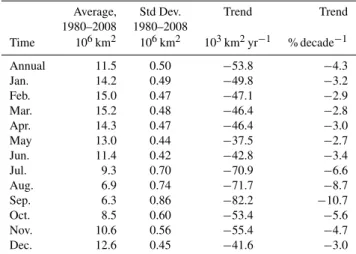
Table 1.Pan-Arctic SIE, 1980–2008. Average values from 1980– 2008, the standard deviation for that period, the trend, and the decadal trend are given for each month. For the trend % per decade, the annual trend and all months reached significance at 99.9 % or greater.
Average, Std Dev. Trend Trend
1980–2008 1980–2008
Time 106km2 106km2 103km2yr−1 % decade−1
Annual 11.5 0.50 −53.8 −4.3
Jan. 14.2 0.49 −49.8 −3.2
Feb. 15.0 0.47 −47.1 −2.9
Mar. 15.2 0.48 −46.4 −2.8
Apr. 14.3 0.47 −46.4 −3.0
May 13.0 0.44 −37.5 −2.7
Jun. 11.4 0.42 −42.8 −3.4
Jul. 9.3 0.70 −70.9 −6.6
Aug. 6.9 0.74 −71.7 −8.7
Sep. 6.3 0.86 −82.2 −10.7
Oct. 8.5 0.60 −53.4 −5.6
Nov. 10.6 0.56 −55.4 −4.7
Dec. 12.6 0.45 −41.6 −3.0
Pacific Quadrant
Russian Quadrant Canadian
Quadrant
Atlantic Quadrant
Study Quadrants
Fig. 1.Study quadrants and sea surface temperature (SST) sam-pling. Quadrant divisions are shown by black longitudinal lines. The rounded box in the Atlantic and Russian quadrants depicts the
sub-region from which SSTs were analyzed: 20◦W to 70◦E, 75◦N to
80◦N.
analyses and used a least squares fit approach and an F-test for confidence intervals.
Our evaluation of sea ice trends identified variations be-tween pan-Arctic (Table 1) and regional sea ice losses (Ta-ble 2). Pan-Arctic summer (July–September) SIE decreased at a more rapid rate (8.7 % per decade – ppd) than late winter (January–March, 3 ppd) from 1980–2008. The Russian and Pacific quadrants had summer SIE decline (9.2 and 9 ppd) similar to the pan-Arctic decline, although the Pacific quad-rant had a much greater September decline (15 ppd). The
Table 2.Regional SIE loss per decade. Trend % per decade calcu-lated for each month for the four quadrants, and annual trend % per decade. Standard typeface represents 95 % significance; italics rep-resent significance of 99 %; bold reprep-resents significance of 99.9 % or greater; and underline represents no significance at 95 %.
Time Atlantic Russian Pacific Canadian
Annual −7.6 −3.7 −3.2 −4.4
Jan. −9.4 −2.7 −0.8 −3.4
Feb. −8.5 −2.2 −1.0 −2.8
Mar. −7.8 −1.4 −1.6 −2.7
Apr. −8.0 −1.7 −2.1 −2.4
May −6.8 −2.4 −1.3 −2.5
Jun. −5 −3.8 −1.2 −4.7
Jul. −6.1 −8.1 −2.4 −10.1
Aug. −6.8 −10.0 −9.6 −7.3
Sep. −6.7 −9.5 −15.0 −6.2
Oct. −5.6 −3.1 −6.5 −6.3
Nov. −7.1 −2.4 −2.7 −7.3
Dec. −9.4 −2.5 −0.7 −2.9
September Sea Ice Extent by Region
Year
SIE
as
Proportion of 1980 S
IE
Pan-Arctic
Canadian Quadrant Pacific Quadrant Atlantic Quadrant
Legend
Russian Quadrant
Fig. 2.September sea ice extent (SIE) by region, 1980–2008. The legend indicates line colors of the different domains in the graph. The graph identifies that Atlantic and Canadian quadrant SIEs are decreasing much slower than the pan-Arctic, while Pacific SIE is decreasing much faster than the pan-Arctic. The Russian quadrant has been decreasing similarly to pan-Arctic trend.
Canadian and Atlantic quadrant summer SIE losses were less rapid (7.9 and 6.5 ppd). Russian, Pacific, and Canadian win-ter SIE losses (2.1, 1.1, and 3 ppd) were similar to pan-Arctic, while the Atlantic quadrant’s winter loss (8.6 ppd) was sig-nificantly more rapid (Fig. 2, Table 2).
the Atlantic quadrant lost annual SIE at almost double the pan-Arctic rate (Tables 1 and 2).
2.2 Arctic sea ice extent and North Atlantic sea surface temperatures
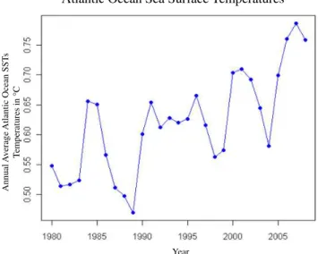
We investigated Atlantic Ocean sea surface temperatures (SSTs) as a possible explanation for the anomalous decrease in winter Atlantic SIE. National Centers for Environmen-tal Prediction (NCEP) and National Center for Atmospheric Research (NCAR) reanalysis data provided Atlantic Ocean temperature values: the average SSTs in degrees Celsius from 75◦N to 80◦N, 20◦W to 70◦E (Fig. 3) (Kalnay et
al., 1996). The NCEP/NCAR SSTs, in turn, were prescribed from Reynolds et al. (2007). Our initial regression analyses of March SIE used a 12-month average of Atlantic Ocean SSTs, with the SSTs preceding March SIE. This regression of Atlantic quadrant SIE had statistical significance at the 99.9 % level (R2= 0.51). Conversely, March SIE in the Pa-cific and Canadian quadrants had no significant correlation with Atlantic SSTs, while Russian and pan-Arctic SIE had a lower correlation with Atlantic SSTs (R2= 0.39 and 0.47, respectively).
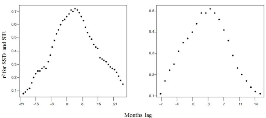
Following the initial test, we ran lead–lag correlations be-tween March SIE and Atlantic Ocean SSTs. The lead–lag correlations consisted of the average of a year’s SSTs, shifted a month with each new correlation. For example, the cen-ter of the lead–lag correlations was October of the previous year’s SSTs to September of the current year’s SSTs, as they relate to March SIE. The next correlation, moving forward, averaged November to October SSTs. If the correlation be-tween SSTs and SIE was symmetric, the strongest correlation should have occurred with the correlation centered on March: October of the previous year through September of the con-current year (e.g., October 1979–September 2008 SSTs re-gressed with March SIE from 1980–2008). Instead, the peak occurred four months later, with February of the concur-rent year to January of the following year (Fig. 4). These two datasets correlated best when the Atlantic Ocean SSTs lagged Atlantic quadrant SIE by several months.
We correlated these variables with de-trended datasets, us-ing the residuals from a linear time series of each dataset. The datasets had the same peak (Fig. 4), indicating that At-lantic region SIE both had a correlation with and preceded changes in North Atlantic SSTs. However, the results do not exclude the possibility that a common driver was responsible for changes in both variables (e.g., air temperatures or deep ocean currents).
Our analysis of regional SIE trends and drivers identified significant sea ice declines across all regions. The Atlantic quadrant’s trends differed substantially from the other quad-rants. Our research points to the likelihood that Atlantic sea ice losses were coupled with and perhaps altered SSTs in the North Atlantic Ocean.
Year
Annual
A
ver
age
Atla
nti
c
Oce
an S
ST
s
T
empera
ture
s
in
°
C
Atlantic Ocean Sea Surface Temperatures
Fig. 3.Atlantic Ocean sea surface temperatures (SST). SST (◦C)
averaged over 75–80◦N, 20◦W–70◦E for the 12 months ending in
February of the indicated year for 1980–2008. For example, 1990 is calculated as March of 1989 through February of 1990.
3 Global climate model performance
In the Coupled Model Inter-comparison Project, Phase 3 (CMIP3) set of simulations, climate models under-simulated the speed with which SIE was diminishing in the Arctic (Stroeve et al., 2007, 2012; Winton, 2011). At the onset of CMIP3, the general expectation was for an ice-free sum-mer Arctic Ocean towards the end of this century based on model simulations; after analyzing the limitations of the sea ice output and the current rate of sea ice decline, sev-eral groups recently estimated an ice-free summer earlier than 2050 (Comiso et al., 2008; Wang and Overland, 2009; Stroeve et al., 2012). Comparison of performance between models offers a guide to those models’ potential for captur-ing the effects of changes in atmospheric and oceanic forc-ing. Improvement of climate models, especially their sea ice components, will be of critical importance in providing the information required to develop sound management strate-gies and informed policy (ACIA, 2005; AMSA, 2009).
Fig. 4.Sea ice extent (SIE) and sea surface temperature (SST) lead lag correlations. March Atlantic SIE correlated with annual average SSTs. At 0, SSTs were averaged from October to September, centered on March of the same year as SIE. Each step forward indicates a one-month lead/lag increment. The left graph has lead–lag correlations squared for the data; the right graph has lead–lag correlations squared for the
detrended data. Correlations (r) are plotted as correspondingr2values to indicate fractions of explained variance.
internal variability, Kay et al. (2011) show that while a 10-yr trend only captured the proper sign of major trends approxi-mately 66 % of the time, a 20-yr time period allows a model to simulate the sign of major trends with 95 % confidence. A 30-yr trend will have a greater likelihood of representing the major trend.
While several studies have evaluated SIE simulation per-formance in climate models (e.g., Zhang and Walsh, 2006), only Overland and Wang (2007) analyzed regional varia-tions in the Arctic. In this study we evaluated the perfor-mance of 13 atmosphere–ocean general circulation models (AOGCMs) in simulating SIE for the period 1980 through 2008 in the Arctic and four sub-regions.
3.1 AOGCM performance evaluation
Model performance was assessed for pan-Arctic SIE and four quadrants from Sect. 2. The AOGCMs used in this research were forced with the A1B emissions scenario. At the release of the IPCC’s AR4, A1B was a middle-of-the-road scenario for emissions. Since that report, global emissions of green-house gases (GHGs) have exceeded all emission scenarios from AR4. Higher emissions are expected to result in more climate forcing than prescribed in these models (IPCC, 2007; Solomon et al., 2009). However, the AOGCMs used observed GHG concentrations for 1980–2000. Because this study cov-ered 1980–2008, we used the emissions scenario for 2001– 2008 (IPCC, 2007; UNMDG, 2010). All forcing scenarios were very similar during this period.
Simulated SIE for 13 models (Table 3) for the histori-cal period 1980–2008 was compared to the observed satel-lite record to develop a performance ranking. The perfor-mance ranking measured accuracy of each model based on three metrics: September SIE trend, March SIE trend, and the absolute value over the annual cycle of SIE. The first two
metrics were analyzed using a least squares linear regression time series for each month’s SIE. The difference between the slope of the regression line for the model output and the observed record was used to rank the simulated March and September trends. The third performance metric, named the absolute error, was based on the 12 calendar-month differ-ences between the observed and modeled SIE from 1980– 2008. The modeled mean value for each month (1980–2008) was subtracted from the observed mean value for that month. Once all monthly differences were computed, the absolute values of the 12 monthly differences were averaged. Each model earned a rank for each metric from 1–13, and the dif-ferent metrics were summed for each model. In this case, a smaller number represented a better rank for the model. These methods were repeated for regional SIE performance to determine which models performed best in each of the four quadrants. The rankings from the four quadrants were also summed to create a combined quadrants rank.
We summarized the pan-Arctic performance of models in Table 4. The models that performed best for the Septem-ber trend simulated the greatest decrease in SeptemSeptem-ber SIE. The INM (Institute for Numerical Mathematics) model had a more rapid trend in September than the observed record, while all other models underestimated the September trend. CCSM estimated a more rapid rate of decline in March than the observed record; all other models underestimated the March trend (Table 3). See full performance results by re-gion in Table 4.
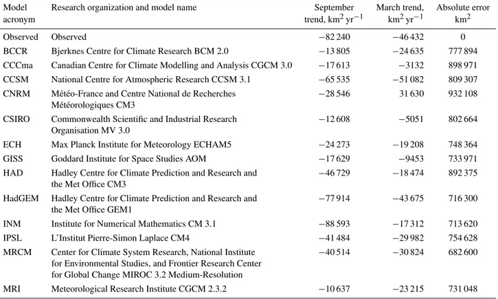
Table 3.Pan-Arctic sea ice models. The model acronyms used in this study, the full names of their research organizations, and the evaluation metrics from this study. The top row displays the observed satellite record and subsequent rows show the output for each model. The third performance metric (absolute error) was based on the 12 calendar-month differences between the observed and modeled SIE from 1980– 2008. The modeled mean value for each month (1980–2008) was subtracted from the observed mean value. Once all monthly differences were computed, the absolute values of the 12 monthly differences were averaged.
Model Research organization and model name September March trend, Absolute error
acronym trend, km2yr−1 km2yr−1 km2
Observed Observed −82 240 −46 432 0
BCCR Bjerknes Centre for Climate Research BCM 2.0 −13 805 −24 635 777 894
CCCma Canadian Centre for Climate Modelling and Analysis CGCM 3.0 −17 613 −3132 898 971
CCSM National Centre for Atmospheric Research CCSM 3.1 −65 535 −51 082 809 307
CNRM M´et´eo-France and Centre National de Recherches −28 546 31 630 932 108
M´et´eorologiques CM3
CSIRO Commonwealth Scientific and Industrial Research −12 608 −5051 802 664
Organisation MV 3.0
ECH Max Planck Institute for Meteorology ECHAM5 −24 273 −19 208 748 364
GISS Goddard Institute for Space Studies AOM −17 629 −9453 733 971
HAD Hadley Centre for Climate Prediction and Research and −46 729 −18 474 892 375
the Met Office CM3
HadGEM Hadley Centre for Climate Prediction and Research and −77 914 −43 675 716 300
the Met Office GEM1
INM Institute for Numerical Mathematics CM 3.1 −88 593 −17 312 713 620
IPSL L’Institut Pierre-Simon Laplace CM4 −41 484 −29 982 754 628
MRCM Center for Climate System Research, National Institute −40 514 −30 824 682 600
for Environmental Studies, and Frontier Research Center for Global Change MIROC 3.2 Medium-Resolution
MRI Meteorological Research Institute CGCM 2.3.2 −10 637 −23 215 731 048
Table 4.GCM performance. The composite ranks of models evaluated in this study, by study region. The models’ order follows pan-Arctic ranking. Each model earns a rank for each metric from 1–13, which is summed to create a composite rank. The first number in each column shows the rank of each model within that region; the number in parentheses is the composite rank.
Pan-Arctic Atlantic Russian Pacific Canadian Combined
quadrants
HadGEM 1 (5) 2 (9) 13 (28) 3 (16) 8 (25) 4 (78)
MRCM 2 (10) 10 (27) 6 (20) 4 (17) 1 (3) 2 (67)
INM 3 (13) 1 (18) 4 (19) 1 (14) 2 (14) 1 (55)
CCSM 4 (15) 13 (32) 9 (25) 11 (26) 8 (25) 13 (108)
IPSL 5 (16) 7 (23) 7 (23) 1 (14) 10 (26) 6 (86)
ECH 6 (21) 11 (28) 1 (10) 12 (27) 6 (24) 9 (89)
HAD 7 (23) 8 (25) 9 (25) 7 (21) 4 (15) 6 (86)
MRI 7 (23) 3 (10) 4 (19) 9 (24) 11 (27) 5 (80)
BCCR 9 (24) 5 (19) 8 (24) 6 (19) 6 (24) 6 (86)
GISS 9 (24) 4 (18) 9 (25) 5 (18) 2 (14) 3 (75)
CSIRO 11 (32) 6 (20) 12 (26) 10 (25) 13 (32) 12 (103)
CNRM 12 (33) 8 (25) 3 (15) 7 (21) 12 (28) 9 (89)
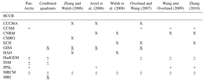
Table 5.Model evaluation synthesis. This table synthesizes model performance over several studies. An X or a + indicates the model was selected by that study. A + indicates the model was among the best five models in our pan-Arctic evaluation. An underline indicates the model performed in the best five models in our combined quadrants evaluation.
Pan- Combined Zhang and Arzel et Walsh et Overland and Wang and Zhang
Arctic quadrants Walsh (2006) al. (2006) al. (2008) Wang (2007) Overland (2009) (2010)
BCCR
CCCMA X X X
CCSM + + + +
CNRM X X X X
CSIRO X
ECH X X X
GISS X X X X
HAD X X
HadGEM + + + + +
INM + +
IPSL + + + +
MRCM + + + + + + + +
MRI X
Projected VS. Observed September SIE
Sea Ice
Ext
ent
in M
il
li
on
Sq. K
m
.
4
5
6
7
8
Fig. 5. Projected vs. observed September sea ice extent (SIE). September SIE from 1980–2008 for the mean of four best perform-ing models in red, the observed SIE in black, and the mean of the remaining nine models in blue.
model. We compared an average of these models to an av-erage of the remaining nine models for their September SIE and trend; while the points for the four-model mean were scattered, their trend line was much closer to the observed record’s trend line than that of the remaining nine models (Fig. 5). Projections from top pan-Arctic models revealed a relatively narrow range of future sea ice scenarios, all of which pointed to the loss of at least two-thirds of 1980 sea ice cover by 2080 (Fig. 6). The MRCM, HadGEM, and CCSM models simulated a complete loss of September sea ice by 2080.
Fig. 6.Pan-Arctic sea ice extent projections, September 2010–2100. Models include CCSM, HadGEM, INM, IPSL, and MRCM.
3.2 AOGCM evaluation study synthesis
sea ice to temperature most closely matched the correspond-ing observational sensitivity durcorrespond-ing 1979–2004.
Our comparison of model performance across these stud-ies indicated that MRCM was the most consistent model: it was selected by every study in our comparison. Five studies selected HadGEM as a top-performing model (Table 5). Of the top four models in our study, INM was the only model not selected by any other study. This model was the only model to overestimate September SIE losses (Table 3). None of the earlier studies included years more recent than 2004, when SIE loss was the most dramatic.
AOGCMs vary in reproducing current sea ice trends. Therefore, it is important to identify models that best simu-late recent SIE and to project future changes with those mod-els. This study found several models that worked best across the Arctic and on regional scales.
4 Arctic marine access
Since 2000, reduced sea ice conditions have resulted in greater Arctic shipping activity and a surge of interest in fu-ture sea ice conditions. Observational records indicated that changes are occurring faster with each decade, such that even the most extreme sea ice simulations from AR4 were not keeping pace (IPCC, 2007; Stroeve et al., 2007, 2012).
The Arctic Marine Shipping Assessment (AMSA) (2009) examined Arctic sea ice observations and model simulations, reviewing social, economic, environmental, and political im-plications of increasing Arctic marine navigation. AMSA used projections from the Hadley Centre GEM1 model for March and September of 2010–2030, 2040–2060, and 2070– 2090. These projections indicated decreasing sea ice condi-tions in the future, with the possibility of a sea ice-free sum-mer by the end of the century. However, several studies have used AOGCM projections to estimate future sea ice condi-tions and found this estimate conservative (Stroeve et al., 2007, 2012; Wang and Overland, 2009; Zhang, 2010).
AMSA investigated Arctic marine access using model pro-jections that, while limited in scope, provided information about the increasing need for safe Arctic transit. This study expanded upon AMSA’s scenarios of Arctic marine accessi-bility by using best-performing AOGCMs to analyze multi-ple future scenarios and to evaluate potential changes in ac-cess to the Arctic Ocean by ice-strengthened vessels through several key passages.
4.1 AOGCM projection analysis
In Sect. 3.1, we identified the models that best simulated sea ice in the Arctic: Hadley Centre Global Environmen-tal Model GEM1 (HadGEM), MIROC Medium Resolution Model (MRCM), Community Climate System Model 3.0 (CCSM), and the Institute of Numerical Mathematics (INM). Nine-year means were constructed for each model for 2030,
2060, and 2090 (2026–2034, 2056–2064, 2086–2094). For comparative purposes, we computed a 9-yr mean of the ob-served sea ice record from 2000 through 2008 based on satel-lite records of sea ice presence (Sect. 2.1). For each 9-yr mean, if the model indicated sea ice presence in a pixel for 5 or more years, the 9-yr mean was classified to have sea ice present.
Because these projections are 9-yr means, they represent what might be expected for normal or median-year condi-tions in 2030, 2060, and 2090. However, significant inter-annual variability exists, such as the extreme minimum of 2007. Even if these opening and closing dates are accurate for a mean year, they are not indicative of the range of sea ice conditions that are possible within the time period shown.
To examine the practicality of these projections, we extrapolated current trends for comparison. The 1980– 2008 time series for September indicated a decrease of 82 240 km2yr−1 (Fig. 8). An extrapolation of this trend to
2030, 2060, and 2090 indicated less SIE than projected by the model averages for 9-yr periods centered on 2030, 2060, and 2090. Further, the 2000–2008 average SIE was less than 1 million km2greater than the 2030 model average. By com-parison, SIE has declined by 2.5 million km2 over the past three decades. The years 2008–2011 have all had less SIE than pre-2007 levels (Stroeve et al., 2012), which implies that SIE will likely continue to decrease at a faster rate than these AOGCMs indicate. However, it is still possible for recently low SIE to be a result of the high natural variability seen in the climate system.
We examined projected Arctic ice-cover, defined as the percent of Arctic seas north of the Arctic Circle with SIE presence, for every month of the 9-yr means centered on 2030, 2060, and 2090. We averaged the projected percent of ice-cover from the four models. This calculation pro-vides insight into the cycle of future SIE decline; our anal-ysis determined significant declines, primarily between July and October, for 2030, 2060, and 2090 (Fig. 9). By 2030, these models projected 90 % or greater ice coverage in win-ter, while September cover decreased to 60 %. The 2060 model projections decreased to 85 % winter cover and less than 40 % September cover. By 2090, the model projections showed less than 85 % winter ice coverage and less than 10 % August–September ice coverage.
4.2 Arctic marine access evaluation
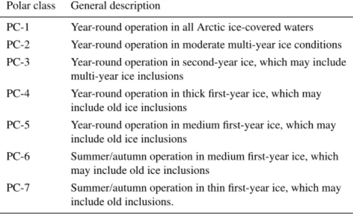
Table 6. The Arctic Guidelines and the Unified Requirements, from AMSA (2009). The Polar Code designates “a system of polar classes for ships with different levels of capability and construction, structural and equipment requirements under various ice conditions. The Unified Requirements apply to ships of member associations constructed on or after March 1, 2008” (AMSA, 2009, p. 56).
Polar class General description
PC-1 Year-round operation in all Arctic ice-covered waters
PC-2 Year-round operation in moderate multi-year ice conditions
PC-3 Year-round operation in second-year ice, which may include
multi-year ice inclusions
PC-4 Year-round operation in thick first-year ice, which may
include old ice inclusions
PC-5 Year-round operation in medium first-year ice, which may
include old ice inclusions
PC-6 Summer/autumn operation in medium first-year ice, which
may include old ice inclusions
PC-7 Summer/autumn operation in thin first-year ice, which may
include old inclusions.
segments of ocean in which sea ice was depicted by satellite imagery or climate models.
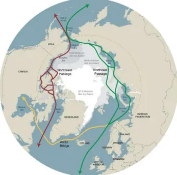
The region and routes evaluated in this study include the Bering Strait, Northeast Passage, Northwest Passage, and Arctic Bridge (Fig. 7). The Bering Strait region separates the Pacific and Arctic Oceans between Russia and Alaska. This region has particular significance to the Arctic, because it provides access to the Arctic Ocean from the Pacific region. It freezes every winter and thaws every summer, a condition which is expected to continue through 2099 in all model out-puts. For the purposes of this study, a route can be considered open if sea ice does not block the route in question. Visually, this means the existence of a corridor of open water along the entire route. However, in the early stages of ice freeze-up or during late stages of thaw, a Polar Class 7 vessel is capable of traversing thin ice; some leeway was required when interpret-ing the results. In some stretches of both the Northwest and Northeast Passages, where the data have only a single pixel of sea ice, the ice may be capable of blocking the entire route. In these cases, we considered a route closed if at least two consecutive pixels of sea ice blocked the route. While trans-port ships can contract icebreakers for escort through these corridors, for the purposes of this study, we considered the route only open if a PC-7 could traverse the route unaided.
The Northeast Passage was defined as a route from the Bering Strait to northern Europe, across the top of Eurasia (Fig. 7). In recent years, most of the Russian coast has be-come ice-free by September, except for the crossing from the Kara Sea to the Laptev Sea. The Northwest Passage “... is the name given to the various marine routes between the Atlantic and Pacific oceans along the north coast of North America that spans the Canadian Arctic Archipelago” (AMSA, 2009). Figure 7 displays several variants of the Northwest Passage. The Arctic Bridge, a proposed future shipping route, starts in
Sea Ice
Ext
ent
in M
il
li
on
Sq. K
m
.
4
5
6
7
8
Observed, Extrapolated, and Modeled Trends
SIE in Million Sq. Km.
Fig. 7.Observed, extrapolated, and modeled Trends. Observed av-erage sea ice extent (SIE) for September 2000–2008; results of the model mean forecasts for September 2030, 2060, 2090; and 1980 observed trends, extrapolated to September 2030, 2060, and 2090.
The x-axis shows SIE, in million km2.
Murmansk, Russia, crosses the Atlantic Ocean, and ends in Churchill, Canada (Fig. 7).
The results for accessibility in the Arctic Ocean are shown in Fig. 10. As indicated previously, “ice-free” is defined as up to 15 % ice cover in the observed record, and therefore pas-sage may require an ice-strengthened vessel such as a PC-7. Under the scenarios in this study, all routes become accessi-ble for longer periods over the course of the century, chang-ing by as much as two months on each end of the season. Most models indicated that the Northwest Passage was inac-cessible in 2030, and one model indicated it was inacinac-cessible in 2060. However, in 2007, and every year since, the North-west Passage was fully navigable for a short period of time. Further, a recent study determined that some routes were al-ready more accessible than these models described for 2030 (Stammerjohn et al., 2012). Since the model-estimated ice-cover for 2030 was similar to current ice-ice-cover, future navi-gation seasons could be longer than suggested by the model simulations.
4
5
6
7
8
Projected Arctic Sea Ice Cover
Per
ce
nt
Ic
e-Cov
ere
d
Fig. 8.Projected Arctic sea ice coverage. Ice coverage of seas within the Arctic Circle by % from January through December for 9-yr model means centered on 2030, 2060, and 2090, averaged over four models.
5 Conclusions
This prototype of an end-to-end assessment of Arctic marine access in the context of changing sea ice cover has assem-bled evaluations of the regional and seasonal trends, drivers, projections, and impacts of Arctic sea ice change. Section 2 highlighted that recent trends of sea ice extent vary region-ally and seasonregion-ally. While the extent to which sea surface temperature anomalies in the Atlantic subarctic drove or re-sulted from sea ice variations could not be established by the correlative analysis performed here, the study made it clear that oceanic coupling must be considered in the diagnosis of North Atlantic sea ice variability and trends. It is important to note that, contrary to our hypothesis, changes in SSTs in the North Atlantic were unlikely to have driven Atlantic SIE changes; changes in North Atlantic SSTs lagged the Atlantic sector SIE.
Section 3 confirmed that global climate models vary in their ability to capture the seasonal amplitude and recent
Fig. 9.Arctic marine navigational routes. The routes depicted are the Northwest Passage, north of Canada; the Northeast Passage, north of Russia; and the Arctic Bridge, which crosses the Atlantic Ocean.
Fig. 10.Arctic accessibility. Projected Arctic marine accessibility from four AOGCMs. A solid line indicates that no models showed accessibility. A long line with a very small dash indicates that one model showed accessibility. A dashed line with equal space cates two models showed accessibility. A sparsely dotted line indi-cates three models showed accessibility. No line indiindi-cates that all models showed accessibility.
trends of Arctic sea ice. Using a three-metric evaluation, we identified the best performing models for the various sectors and for the Arctic as a whole. Our synthesis of GCM perfor-mance evaluations indicated that, regardless of methodology, several models consistently performed well.
access through the 21st century. While this study could not guarantee that models with the best hindcast success will produce the most credible projections for the coming decades, we found no justification for reliance on models with poorer track records in their simulated seasonal cycles and trends. Scenarios obtained from the subset of the four best-performing models pointed to a lengthening open wa-ter season, and hence the period of marine access, by one to three months in the navigation corridors considered here. This assessment suggests that the Northwest and Northeast Passages hold potential for enhanced marine access to the Arctic in the future, including shipping and resource devel-opment opportunities.
We accompany this assessment with a crucial question and caution: does the extreme sea ice retreat observed during 2007–2011 represent natural variability, or is it an indicator that models are not sensitive enough to external forcing on Arctic sea ice? While 2007–2011 SIE levels could be due to natural variability, several studies (Johannessen et al., 1999; Hilmer and Jung, 2000; Comiso et al., 2008) have suggested that, in the last two decades, the sea ice regime has shifted, resulting in faster SIE decline. Previous studies (Stroeve et al., 2007, 2012; Zhang, 2010), as well as our analyses in Sects. 3.1 and 4.2, point to the conclusion that while GCMs can reproduce historic trends with some accuracy, they are not keeping pace with the observed trends of the past decade. Future analyses could extend the work of this study in several ways. Most importantly, new models from the IPCC Fifth Assessment are becoming available. Future generations of models will provide finer resolution to more accurately de-fine Arctic regions and marine routes, and to achieve greater precision in determining when those navigation routes might be accessible. In particular, accessibility should be deter-mined on a sub-monthly basis. Finally, as more realistic ice thickness distributions become available, assessments of fu-ture changes in marine access could be performed for mul-tiple types of Polar Class vessels; the primary difference be-tween PC-5 and lower vessels is the thickness of ice they are capable of traversing. A detailed assessment, including evaluation of multiple Polar Class designations, will be im-perative as the development of the Arctic matures and natural resource extraction and associated commerce increases.
Acknowledgements. We thank William Chapman for his help in
re-trieving the National Snow and Ice Data Center sea ice data and for providing the National Centers for Environmental Prediction and National Center for Atmospheric Research reanalysis ocean sea sur-face temperature data. Thanks to Tom Kurkowski and Dustin Rice for data management and analysis support, Kristin Timm for Fig. 9, and Sherry Modrow and Steven Seefeldt for their additional reviews. This work was supported by the National Science Founda-tion’s Office of Polar Programs through Grant ARC-1023131, the Alaska Climate Science Center, through Cooperative Agreement Number G10AC00588 from the United State Geological Survey, and by the University of Alaska, Fairbanks Scenarios Network for
Alaska and Arctic Planning (SNAP; www.snap.alaska.edu). The contents are solely the responsibility of the authors and do not necessarily represent the official views of USGS. All statistical analyses were performed using the R language and environment for statistical computing and graphics. For more information, see http://www.r-project.org/.
Edited by: J. Stroeve
References
ACIA – Arctic Climate Impact Assessment: available at: http:// www.acia.uaf.edu, last access: 26 March 2012, Cambridge Uni-versity Press, Cambridge, 1024 pp., 2005.
AMSA – Arctic Marine Shipping Assessment: 2009 Report, avail-able at: http://www.pame.is/amsa, last access: 26 March 2012, Arctic Council, Norwegian Chairmanship, Oslo, Norway, April 2009.
Arzel, O., Fichefet, T., and Goosse, H.: Sea ice evolution over the 20th and 21st centuries as simulated by current AOGCMs, Ocean Model., 12, 401–415, 2006.
Cavalieri, D., Parkinson, C., Gloersen, P., and Zwally, H. J.: Sea ice concentrations from Nimbus-7 SMMR and DMSP SSM/I pas-sive microwave data (1980–2007), National Snow and Ice Data Center, Digital Media, updated 2008, Boulder, CO, USA, 1996. Comiso, J., Parkinson, C., Gersten, R., and Stock, L.: Accelerated
decline in the Arctic sea ice cover, Geophys. Res. Lett., 35, L01703, doi:10.1029/2007GL031972, 2008.
Fetterer, F., Knowles, K., Meier, W., and Savoie, M.: Sea Ice Index, National Snow and Ice Data Center, Digital Media, Boulder, CO, USA, 2009.
Francis, J. and Hunter, E.: Drivers of declining sea ice in the Arc-tic winter: a tale of two seas, Geophys. Res. Lett., 34, L17503, doi:10.1029/2007GL030995, 2007.
Hilmer, M. and Jung, T.: Evidence for a recent change in the link between the North Atlantic Oscillation and the Arctic sea ice export, Geophys. Res. Lett., 27, 989–992, doi:10.1029/1999GL010944, 2000.
IPCC: Climate Change 2007: the Physical Science Basis – Con-tribution of Working Group I to the Fourth Assessment Re-port, 15 IPCC Model Documentation: CMIP3 climate model documentation, references, and links, Intergovernmental Panel on Climate Change, available at: http://www-pcmdi.llnl.gov/ ipcc/model documentation/ipcc model documentation.php, last access: 26 July 2011, Cambridge University Press, Cambridge, 2007.
Johannessen, O., Shalina, E., and Miles, M.: Satellite evidence for an Arctic sea ice cover in transformation, Science, 286, 5446, doi:10.1126/science.286.5446.1937, 1999.
Kalnay, E., Kanamitsu, M., Kistler, R., Collins, W., Deaven, D., Gandin, L., Iredell, M., Saha, S., White, G., Woollen, J., Zhu, Y., Leetmaa, A., and Reynolds, R.: The NCEP/NCAR 40-year reanalysis project, B. Am. Meteorol. Soc., 77, 437–472, 1996. Kay, J. E., Holland, M. M., and Jahn, A.: Inter-annual to
Meier, W., Fetterer, F., Knowles, K., Meier, W., Savoie, M., and Brodzik, M. J.: Sea ice concentrations from Nimbus-7 SMMR and DMSP SSM/I passive microwave data (2008), National Snow and Ice Data Center, updated quarterly, Digital Media, Boulder, CO, USA, 2006.
Meier, W., Stroeve, J., and Fetterer, F.: Whither Arctic sea ice? A clear signal of decline re-gionally, seasonally, and extending be-yond the satellite record, Ann. Glaciol., 46, 428–434, 2007. Overland, J. and Wang, M.: Future regional Arctic sea ice declines,
Geophys. Res. Lett., 34, L17705, doi:10.1029/2007GL030808, 2007.
Overland, J., Wang, M., Bond, N., Walsh, J., Kattsov, V., and Chap-man, W.: Considerations in the selection of global climate mod-els for regional climate projections: the Arctic as a case study, J. Climate, 24, 1583–1597, doi:10.1175/2010JCLI3462.1, 2011. Parkinson, C. and Cavalieri, D.: Arctic sea ice variability
and trends, 1979–2006, J. Geophys. Res., 113, C07003, doi:10.1029/2007JC004558, 2008.
Parkinson, C., Cavalieri, D., Gloersen, P., Zwally, H., and Comiso, J.: Arctic sea ice extents, areas, and trends, 1978–1996, J. Geophys. Res., 104, 20837–20856, doi:10.1029/1999JC900082, 1999.
Perovich, D., Meier, W., Maslanik, J., and Richter-Menge, J.: Sea Ice Cover (in Arctic Report Card 2010), available at: http://www. arctic.noaa.gov/reportcard (last access: 20 February 2013), 2010. Polyak, L., Alley, R., Andrews, J., Brigham-Grette, J., Cronin, T., Darby, D., Dyke, A., Fitzpatrick, J., Funder, S., Holland, M., Jennings, A., Miller, G., O’Regan, M., Savelle, J., Ser-reze, M., St. John, K., White, J., and Wolf, E.: History of sea ice in the Arctic, Quarternary Sci. Rev., 29, 1757–1778, doi:10.1016/j.quascirev.2010.02.010, 2010.
Reynolds, R. W., Smith, T., Liu, C., Chelton, D., Casey, K., and Schlax, M.: Daily high-resolution blended analyses for sea sur-face temperature, J. Climate, 20, 5473–5496, 2007.
Shimada, K., Kamoshida, T., Itoh, M., Nishino, S., Carmack, E., McLaughlin, F., Zimmerman, S., and Proshutinsky, A.: Pacific Ocean inflow: influence on catastrophic reduction of sea ice cover in the Arctic Ocean, Geophys. Res. Lett., 33, L08605, doi:10.1029/2005GL025624, 2006.
Solomon, S., Plattner, G., Knutti, R., and Friedlingstein,
P.: Irreversible climate change due to carbon dioxide
emissions, P. Natl. Acad. Sci. USA, 106, 1704–1709, doi:10.1073/pnas.0812721106, 2009.
Stammerjohn, S., Massom, R., Rind, D., and Martinson, D.: Regions of rapid sea ice change: an inter-hemispheric seasonal comparison, Geophys. Res. Lett., 39, L06501, doi:10.1029/2012GL050874, 2012.
Stroeve, J., Holland, M., Meier, W., Scambos, T., and Serreze, M.: Arctic sea ice decline: faster than forecast, Geophys. Res. Lett., 34, L095101, doi:10.1029/2007GL029703, 2007.
Stroeve, J., Serreze, M., Holland, M., Kay, J., Malanik, J., and Barrett, A.: The Arctic’s rapidly shrinking sea ice cover: a research synthesis, Climatic Change, 110, 1005–1027, doi:10.1007/s10584-011-0101-1, 2012.
UNMDG – United Nations Statistics Division: Millennium Development Goals Indicators: Carbon Dioxide Emissions
(CO2), available at: http://mdgs.un.org/unsd/mdg/SeriesDetail.
aspx?srid=749&crid= (last access: 26 July 2011), 2010. Walsh, J., Chapman, W., Romanovsky, V., Christensen, J., and
Sten-del, M.: Global climate model performance over Alaska and Greenland, J. Climate, 21, 6156–6174, 2008.
Wang, M. and Overland, J. E.: A sea ice free summer Arc-tic within 30 years?, Geophys. Res. Lett., 36, L07502, doi:10.1029/2009GL037820, 2009.
Winton, M.: Do climate models underestimate the sensitivity of Northern Hemisphere sea ice cover?, J. Climate, 24, 3924–3934, doi:10.1175/2011JCLI4146.1, 2011.
Zhang, X.: Sensitivity of Arctic summer sea ice coverage to global warming forcing: towards reducing uncertainty in Arctic climate change projections, Tellus A, 62, 220–227, 2010.