The Cryosphere, 6, 1383–1394, 2012 www.the-cryosphere.net/6/1383/2012/ doi:10.5194/tc-6-1383-2012
© Author(s) 2012. CC Attribution 3.0 License.
The Cryosphere
Constraining projections of summer Arctic sea ice
F. Massonnet1, T. Fichefet1, H. Goosse1, C. M. Bitz2, G. Philippon-Berthier1,3, M. M. Holland4, and P.-Y. Barriat1
1Georges Lemaˆıtre Centre for Earth and Climate Research, Earth and Life Institute, Universit´e catholique de Louvain,
Louvain-la-Neuve, Belgium
2Department of Atmospheric Sciences, University of Washington, Seattle, WA, USA 3Laboratoire des Sciences du Climat et de l’Environnement, Gif-sur-Yvette, France 4National Center for Atmospheric Research, Boulder, CO, USA
Correspondence to:F. Massonnet ([email protected])
Received: 7 July 2012 – Published in The Cryosphere Discuss.: 27 July 2012
Revised: 2 November 2012 – Accepted: 5 November 2012 – Published: 22 November 2012
Abstract. We examine the recent (1979–2010) and future (2011–2100) characteristics of the summer Arctic sea ice cover as simulated by 29 Earth system and general cir-culation models from the Coupled Model Intercomparison Project, phase 5 (CMIP5). As was the case with CMIP3, a large intermodel spread persists in the simulated summer sea ice losses over the 21st century for a given forcing sce-nario. The 1979–2010 sea ice extent, thickness distribution and volume characteristics of each CMIP5 model are dis-cussed as potential constraints on the September sea ice ex-tent (SSIE) projections. Our results suggest first that the fu-ture changes in SSIE with respect to the 1979–2010 model SSIE are related in a complicated manner to the initial 1979– 2010 sea ice model characteristics, due to the large diversity of the CMIP5 population: at a given time, some models are in an ice-free state while others are still on the track of ice loss. However, in phase plane plots (that do not consider the time as an independent variable), we show that the transition towards ice-free conditions is actually occurring in a very similar manner for all models. We also find that the year at which SSIE drops below a certain threshold is likely to be constrained by the present-day sea ice properties. In a sec-ond step, using several adequate 1979–2010 sea ice metrics, we effectively reduce the uncertainty as to when the Arc-tic could become nearly ice-free in summertime, the interval [2041, 2060] being our best estimate for a high climate forc-ing scenario.
1 Introduction
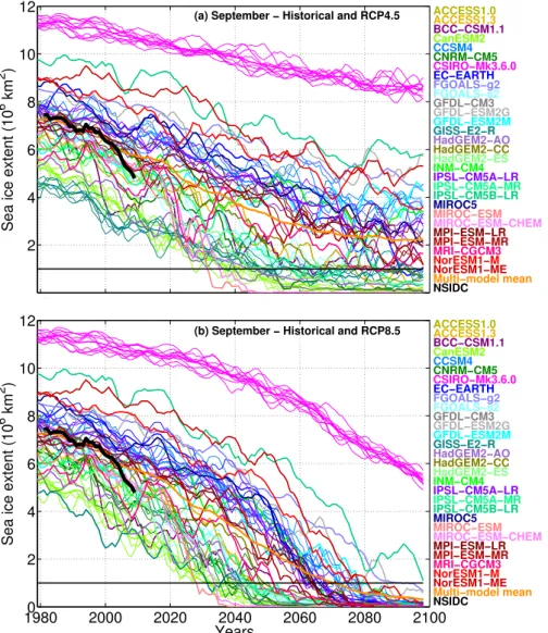
The evolution of summer Arctic sea ice in the next decades is of particular economic, ecological and climatic relevance (ACIA, 2005). Indeed, the area of surviving Arctic sea ice at the end of the melt season (in September) determines in large part the proportion of seasonal, first-year ice in the fol-lowing months (Armour et al., 2011; Maslanik et al., 2007). Given that the shift towards a full first-year sea ice regime would have important implications (AMAP, 2011), the re-cent observed dramatic sea ice retreats in late summer (2005, 2007, 2008, 2011; Fetterer et al., 2012) stress the urgent need for extracting reliable information from the abundant exist-ing projections of Arctic sea ice. Here we examine the 21st century projections of summer Arctic sea ice from 29 Earth system and general circulation models (ESMs and GCMs) participating in the Coupled Model Intercomparison Project, phase 5 (CMIP5, http://pcmdi3.llnl.gov/esgcet). All these models project a decline in summer Arctic sea ice extent over the next decades for medium and high forcing scenarios (Fig. 1).
potential drawbacks. In the former, one needs to identify a reasonable criterion for selection and, if the models are to be combined collectively, a sound multi-model weighting rule. In the latter, one has to work with the hypothesis that the recalibration is physically robust and meaningful, given that the different models are often in very different states.
To the best of our knowledge, only four studies have made use of the CMIP5 output of Arctic sea ice so far. Pavlova et al. (2011) focused on the recent model properties and showed that the 1980–1999 Arctic mean sea ice extent in CMIP5 models is closer to reality than for CMIP3, in both winter and summer. Stroeve et al. (2012) also reported that the Arc-tic sea ice extent properties are better reproduced with the CMIP5 models; their results suggest, in line with other recent studies (e.g. Notz and Marotzke, 2012), that the role of ex-ternal forcings on the simulated and observed summer Arctic sea ice retreat is becoming increasingly clear. In a recent re-view, Maslowski et al. (2012) describe the recent Arctic sea ice properties simulated by 8 CMIP5 models and point out that large biases still remain compared to CMIP3. For ex-ample, 4 of the 8 CMIP5 models considered in this study display an unrealistic summer sea ice thickness distribution. Finally, Wang and Overland (2012) make a CMIP5 model se-lection based on the climatological sea ice extent properties and adjust the summer sea ice extents of these models to the observed value as to narrow the large spread present among the different integrations.
In this work, we focus on the summer Arctic sea ice pro-jections and show that several variables related to the cur-rent 1979–2010 sea ice state are influencing the most recent generation of summer Arctic sea ice projections. Long-term means of September sea ice extent, amplitude of the seasonal cycle of sea ice extent, annual mean sea ice volume and trend in September sea ice extent are considered as metrics to con-strain sea ice projections. In our selection, we take into ac-count the effects of internal variability – particularly large for the trend – as to not reject models for wrong reasons. In this paper, we also identify that the transition from stable, pre-industrial states to seasonally (near) ice-free conditions is marked by a nonlinear relationship between the mean and the trend in September sea ice extent. This strengthens the idea that simulating a reasonable sea ice state over the recent decades is a necessary condition to limit biases in summer Arctic sea ice projections.
Section 2 presents the CMIP5 archive, how sea ice-related quantities were derived from the outputs and the reference products that we use for model selection. In Sect. 3, we re-late the present-day sea ice properties in the CMIP5 mod-els to their future behaviour, and present our model selection procedure. We discuss this selection and its implications in the Discussion (Sect. 4) and close the paper by a conclusion.
2 Model output and observational data
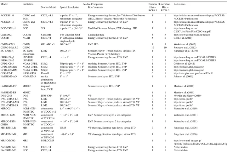
Table 1 lists the 29 ESMs and GCMs used for this study, selected on the requirement that they archive sea ice fields up to 2100 (a final sample of ∼35 models is expected when all simulations are uploaded onto the repository). Out of the existing climate forcing scenarios, we only retain two “representative concentration pathways” (RCPs, Moss et al., 2010): RCP4.5 and RCP8.5. The radiative forcing in RCP8.5 increases nearly steadily over the 21st century to peak at+8.5 W m−2in 2100 relative to pre-industrial levels. In RCP4.5, the increase is also nearly linear up to 2060, and then eventually flattens out so that a net value of+4.5 W m−2 is reached in 2100 (van Vuuren et al., 2011). Because of the much smaller population of available models under RCP2.6 and RCP6.0, these two other scenarios are not discused here. For each simulation, we derive three quantities from the monthly sea ice fields on the model native grid: the sea ice extent (calculated as the area of grid cells comprising at least 15 % of ice); the total sea ice volume (sum, over the grid cells, of the grid cell area multiplied by the mean thickness including open water), and the thin ice extent, which is the extent of sea ice with mean grid cell thickness between 0.01 and 0.5 m. Working on the original grid is a well-founded choice, (1) because the grid is part of the model experimental design, and (2) because no ice is artificially created/removed due to interpolation onto a common grid, with a prescribed land-sea mask. However, as the area covered by ocean in the Arctic (defined here north of 65◦N) is different on each model grid (∼1.8 million km2 difference between the ex-tremes), care must be taken when the output is analysed: for example, a model may misrepresent the observed sea ice ex-tent due to too coarse a grid resolution or to an inaccurate representation of coastlines and land distribution. We there-fore consider the land-sea mask as an important property of the CMIP5 simulations.
Here the term “CMIP5 model” refers to each of the 29 ESMs and GCMs listed in Table 1. If a model comprises several members, then an equally weighted average of these members is considered, but the distribution of the members is still displayed. Therefore, for models with members, we use the mean of the members to evaluate the average character-istics of this model, the scatter of the ensemble providing in-formation on the possible contribution of internal variability in additional analyses. For the other models, the information relies on the only one available realization. The multi-model mean is obtained in two steps. First, the members are aver-aged for each CMIP5 model. If a model only comprises one member, then this single member is considered. Then the av-erage is taken with equal weight over all the models. In this sense, the multi-model mean is not biased towards models with more members.
19800 2000 2020 2040 2060 2080 2100 2
4 6 8 10 12
Years
Sea ice extent (10
6 km 2 )
Northern Hemisphere September Sea ice extent (historical_rcp45)
19800 2000 2020 2040 2060 2080 2100
2 4 6 8 10 12
Years
Sea ice extent (10
6 km 2 )
Northern Hemisphere September Sea ice extent (historical_rcp85)
ACCESS1.0 ACCESS1.3
BCC−CSM1.1
CanESM2 CCSM4 CNRM−CM5
CSIRO−Mk3.6.0 EC−EARTH FGOALS−g2
FGOALS−s2
GFDL−CM3 GFDL−ESM2G
GFDL−ESM2M GISS−E2−R
HadGEM2−AO
HadGEM2−CC HadGEM2−ES INM−CM4
IPSL−CM5A−LR IPSL−CM5A−MR IPSL−CM5B−LR MIROC5 MIROC−ESM MIROC−ESM−CHEM MPI−ESM−LR MPI−ESM−MR MRI−CGCM3 NorESM1−M NorESM1−ME Multi−model mean NSIDC
(a) September − Historical and RCP4.5
(b) September − Historical and RCP8.5
Fig. 1.September Arctic sea ice extent (5-yr running mean) as simulated by 29 CMIP5 models. The historical runs are merged with the RCPs (representative concentration pathways, Moss et al., 2010) 4.5(a)and 8.5(b)runs. Members of a same model, if any, are represented by thin lines. Individual models (or the mean of all their members, if any) are represented by thick lines. The multi-model mean (equal weight for each model) is depicted by the thick orange line. Observations (Fetterer et al., 2012) are shown as the thick black line. The horizontal black line marks the 1 million km2September sea ice extent threshold defining ice-free conditions in this paper.
calculated on a polar stereographic 25 km resolution grid, with the same 15 % cutoff definition as that described above. We also use the Pan-Arctic Ice Ocean Modeling and Assimi-lation System (PIOMAS, Schweiger et al., 2011) output for sea ice volume estimates. This Arctic sea ice reanalysis is obtained by assimilation of sea ice concentration and sea sur-face temperature data into an ocean–sea ice model. We use an adjusted time series of sea ice volume partly accounting for the possible thickness biases in the reanalysis (A. Schweiger, personal communication, 2012). We perform the comparison to observations and to the reanalysis over the 1979–2010 ref-erence period. For that purpose, we have extended the 1979– 2005 available CMIP5 sea ice output from the historical sim-ulations with the 2006–2010 fields under RCP4.5. At such
short time scales and so early in the 21st century, the choice of the scenario to complete the 1979–2005 time series is of no particular importance (not shown).
3 Results
Table 1.The 29 CMIP5 models used in the study, and the principal characteristics of their sea ice components.
Model Institution Sea Ice Component Number of members References Sea Ice Model Spatial Resolution Brief contents Hist – Hist –
RCP4.5 RCP8.5
ACCESS1.0 CSIRO and CICE, v4.1 tripolar, 1◦×1◦, Energy-conserving thermo, Ice Thickness Distribution 1 1 http://wiki.csiro.au/confluence/display/ACCESS/ BOM refinement at equator (ITD), Elastic-Viscous-Plastic (EVP) rheology ACCESS+Publications
ACCESS1.3 CSIRO and CICE, v4.1 tripolar, 1◦×1◦, Energy-conserving thermo, ITD, EVP 1 1 http://wiki.csiro.au/confluence/display/ACCESS/
BOM refinement at equator ACCESS+Publications
BCC-CSM1-1 BCC SIS tripolar,1◦×(1–1/3)◦ Modified Semtner 3-layer; EVP rheology; ITD 1 1 http://www.lasg.ac.cn/ C20C/UserFiles/File/C20C-xin.pdf CanESM2 CCCma CanSIM1 T63 Gaussian Grid Cavitating fluid 5 5 http://www.cccma.ec.gc.ca/models CCSM4 NCAR CICE, v4 1◦orthogonal rotated, Energy-conserving thermo, ITD, EVP 5 6 Gent et al. (2011)
displaced pole
CNRM-CM5 CNRM GELATO v5 ORCA-1◦ EVP, ITD 1 5 Voldoire et al. (2012)
CSIRO-Mk6.3.0 CSIRO 10 10 Rotstayn et al. (2012)
EC-EARTH EC-Earth LIM2 ORCA-1◦ Semtner 3 layer+brine pockets, virtual ITD, 1 1 Hazeleger et al. (2010) consortium Viscous-Plastic (VP) rheology
FGOALS-g2 IAP-THU CICE, v4 ∼1×1◦ Energy-conserving thermo, ITD, EVP 1 1 http://www.lasg.ac.cn/FGOALS/CMIP5
FGOALS-s2 IAP-THU 3 3 http://www.lasg.ac.cn/FGOALS/CMIP5
GFDL-CM3 NOAA GFDL SISp2 Tripolar grid∼1◦×1◦ modified Semtner 3-layer, ITD, EVP 1 1 Griffies et al. (2011) GFDL-ESM2G NOAA GFDL SISp2 Tripolar grid∼1◦×1◦ modified Semtner 3-layer, ITD, EVP 1 1 http://nomads.gfdl.noaa.gov/ GFDL-ESM2M NOAA GFDL SISp2 Tripolar grid∼1◦×1◦ modified Semtner 3-layer, ITD, EVP 1 1 http://nomads.gfdl.noaa.gov/ GISS-E2-R NASA GISS Russell 1◦×1.25◦ 5 1 http://data.giss.nasa.gov/modelE/ar5/ HadGEM2-AO NIMR/KMA sea ice 1◦×1◦ Semtner zero layer, ITD, EVP 1 1 Johns et al. (2006)
component of HadGOM2
HadGEM2-CC MOHC inspired Semtner zero layer, ITD, EVP 1 1 Martin et al. (2011) from CICE
HadGEM2-ES MOHC 1 1 Martin et al. (2011)
INM-CM4 INM INM-CM4 1◦×0,5◦ VP 1 1 Volodin and Gusev (2010) IPSL-CM5A-LR IPSL LIM2 ORCA-2◦ Semtner 3 layer+brine pockets, virtual ITD, VP 3 3 http://icmc.ipsl.fr/ IPSL-CM5A-MR IPSL LIM2 ORCA-2◦ Semtner 3 layer+brine pockets, virtual ITD, VP 1 1 http://icmc.ipsl.fr/ IPSL-CM5B-LR IPSL LIM2 ORCA-2◦ Semtner 3 layer+brine pockets, virtual ITD, VP 1 1 http://icmc.ipsl.fr/ MIROC5 AORI-NIES- component 1.4◦×(0.5◦–1.4◦) 1 1 Watanabe et al. (2010)
JAMSTEC of COCO v4.5
MIROC-ESM AORI-NIES- component ∼1,4◦×1◦, L44 EVP, Semtner zero layer, 2 ice categories 1 1 Watanabe et al. (2011) JAMSTEC of COCO3.4
MIROC-ESM- AORI-NIES- component ∼1,4◦×1◦, L44 EVP, Semtner zero layer, 2 ice categories 1 1 Watanabe et al. (2011) CHEM JAMSTEC of COCO3.4
MPI-ESM-LR MPI component GR15 VP rheology, Semtner zero-layer, virtual ITD 3 3 Jungclaus et al. (2006) of MPI-OM
MPI-ESM-MR MPI component ∼0,4◦×0,4◦ VP rheology, Semtner zero-layer, virtual ITD 1 1 Jungclaus et al. (2006) of MPI-OM
MRI-CGCM3 MRI MRI.COM3 1 1 http://www.mri-jma.go.jp/
Publish/Technical/DATA/VOL 64/tec rep mri 64.pdf NorESM1-ME NCC CICE, v4 Energy-conserving thermo, ITD, EVP 1 1 Not available
NorESM1-ME NCC CICE, v4 Energy-conserving thermo, ITD, EVP 1 1 Not available
Note: this table has been filled with as much information as possible (July 2012). A full documentation about the models is expected soon from the CMIP5 consortium.
SSIE crosses a given threshold is linearly related to the base-line state (Sect. 3.3). This motivates the model selection in-troduced in Sect. 3.4.
3.1 1979–2100 simulated September sea ice extent
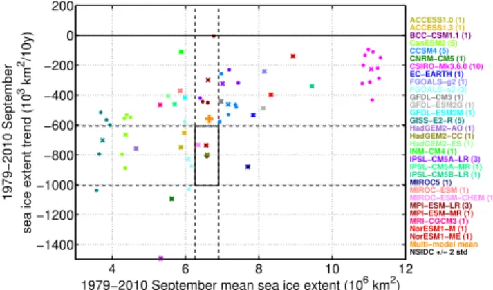
A summary of the summer Arctic sea ice extent characteris-tics simulated by the 29 CMIP5 models and their members is shown in Fig. 2 for the 1979–2010 reference period. We make the distinction between the climatological mean state (x-axis) and the linear trend (y-axis) over that period. The multi-model mean compares well with the observed SSIE (x-axis). The distribution of the extents among CMIP5 models is roughly symmetric about the multi-model mean, with one notable outlier (CSIRO-Mk3.6.0). The width of the distri-bution is substantial (∼7 million km2) and has not narrowed since CMIP3 (Parkinson et al., 2006).
The CMIP5 multi-model mean trend underestimates the observed trend (y-axis in Fig. 2) in magnitude. However the observations lie inside the distribution of the modeled trends (as an ensemble), and hence, the models as a whole cannot be considered inconsistent with the observed trend. The same is true for CMIP3 models for the 1979–2006 period as shown
by Stroeve et al. (2007). It is worth noting that the magni-tude of the SSIE trend of the multi-model mean for 1979– 2006 is considerably higher in the CMIP5 models compared to CMIP3 models (not shown here), suggesting that model improvements or tuning have caused models to have greater sea ice decline in September (see also Stroeve et al., 2012, for a detailed analysis of the CMIP5 model trends in summer Arctic sea ice extent).
All the models examined in this study project a decline in the summer sea ice extent over the present century (Fig. 1). Consistently, the response is faster for individual models and the multi-model mean under the higher emission scenario (RCP8.5). Still, the spread in the projections remains large. For both scenarios, the September sea ice extent during a par-ticular decade of the 21st century and the decade at which an ice-free Arctic could be realized, are highly uncertain quan-tities if all models are considered.
3.2 Relating present-day sea ice to projected losses
4 6 8 10 12 −1400
−1200 −1000 −800 −600 −400 −200 0 200
1979−2010 September mean sea ice extent (106 km2)
1979−2010 September
sea ice extent trend (10
3 km 2/10y)
1979−2010 September Northern Hemisphere sea ice extent
ACCESS1.0 (1)
ACCESS1.3 (1)
BCC−CSM1.1 (1) CanESM2 (5) CCSM4 (5) CNRM−CM5 (1)
CSIRO−Mk3.6.0 (10) EC−EARTH (1)
FGOALS−g2 (1)
FGOALS−s2 (3)
GFDL−CM3 (1)
GFDL−ESM2G (1)
GFDL−ESM2M (1)
GISS−E2−R (5) HadGEM2−AO (1)
HadGEM2−CC (1)
HadGEM2−ES (1)
INM−CM4 (1)
IPSL−CM5A−LR (3)
IPSL−CM5A−MR (1)
IPSL−CM5B−LR (1)
MIROC5 (1) MIROC−ESM (1) MIROC−ESM−CHEM (1) MPI−ESM−LR (3) MPI−ESM−MR (1) MRI−CGCM3 (1) NorESM1−M (1) NorESM1−ME (1) Multi−model mean NSIDC +/− 2 std
Fig. 2.1979–2010 mean of (x-axis) and trend in (y-axis) September Arctic sea ice extent, as simulated by the CMIP5 models and their members. Members of a same model (if any) are represented by dots (•). Individual models (or the mean of all their members, if any) are represented by crosses (×). The number of members for each model is indicated in parentheses. The multi-model mean is depicted as the orange plus (+). Observations (Fetterer et al., 2012) are shown as the black dot, with±2σ windows for the mean and trend estimates (dashed lines). The values ofσare calculated as the standard deviation of the 1979–2010 SSIE time series divided by the square root of the number of observations (32) for the mean, and as the standard deviation estimate of the slope of the 1979–2010 SSIE linear fit.
a relationship could exist between the two time periods is not clear: with the CMIP3 data set, Arzel et al. (2006) showed that the summer mean 1981–2000 extent influences the rel-ative (i.e. in %) but not the absolute changes in SSIE. How-ever, a relationship can be found by construction even if the mean X and the projected changes 1X are actually inde-pendent. In addition, they found no relationship between the 1981–2000 mean sea ice thickness and future SSIE changes. On the other hand, Holland et al. (2008) found that the base-line thickness of ice is well correlated with the SSIE through-out the 21st century. Using the CMIP2 data set, Flato (2004) – using annual mean values of Arctic sea ice extent – reported that the initial extent does not strongly impact future changes in sea ice extent; this is consistent with the hypothesis that, if such relationships exist, they may be seasonally dependent (Bitz et al., 2012). Bo´e et al. (2009) found that the future re-maining SSIE correlates well with the 1979–2007 trends in SSIE and the area of thin (0.01–0.5 m) ice over 1950–1979, but again they worked with relative values. Moreover, the re-lationship involving the 1950–1979 thin ice area does not necessarily hold over the more recent (1979–2007) period. To summarize, it is not clear to date whether or not a rela-tionship may exist between the present-day (1979–2010) sea ice cover and its projected changes. Below we propose re-viewing, without ambiguity, the possible existence or not of such mechanisms in the most recent generation of climate models.
With the CMIP5 data set, there is no clear and robust linear relationship between the 1979–2010 sea ice characteristics and the projected changes in SSIE at a given time period. As an example (left part of Table 2), across the CMIP5 models, the correlation between (1) the mean 1979–2010 SSIE (pre-dictor I in Table 2) and (2) the SSIE change between 1979– 2010 and 2030–2061 (the predictand) under RCP4.5 is 0.38 (significant atp <0.05) but drops to 0.20 (non-significant at
p <0.05) for 2069–2100. The other correlations given in the left part of Table 2 are not convincing: when they are signif-icant, the sign of the relationship is found to be scenario and time period-dependent as illustrated when ice volume is used as a predictor.
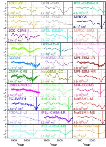
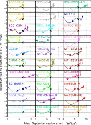
To help understand this issue, we show in Fig. 3 the run-ning trend in SSIE for all CMIP5 models for RCP8.5. As sug-gested in the figure, the trends, and thus the sea ice changes, become increasingly large sometime during the 21st century, and then go to zero. The timing of the most negative trend is marked with a vertical bar in the figure, and is clearly model-dependent. To gain further insight into this, we dis-play in Fig. 4 the evolution of SSIE trends as a function of the mean SSIE, in order to visualize the dynamics of the sys-tem. In these “phase-plane” plots (a variable versus its time derivative), clear similarities come to light. All models fol-low a similar trajectory: they start from the right, with rel-atively high mean SSIE at the beginning of the simulation. Then they move leftwards as the mean SSIE decreases and all experience a U-shaped trajectory as the mean SSIE de-creases further to ice-free conditions (the 2030–2061 posi-tion of each model is marked with a colored dot). In Fig. 4, the spread in the CMIP5 population is thus represented by the different 1979–2010 positions of the CMIP5 models on their trajectories (colored crosses): for example, BCC-CSM1.1, CanESM2 and GISS-E2-R are already near the minimum, while EC-EARTH and CCSM4 have not reached it yet. Un-der RCP4.5, similar trajectories exist (supplement figure) for the subset of models that reach ice-free conditions in September by∼2060 – the approximate year at which the RCP4.5 forcing stabilizes – suggesting that, as long as the SSIE reaches (near) ice-free conditions under the effect of increased radiative forcing, the U-shaped trajectory occurs.
3.3 Relating present-day sea ice to year of disappearance
To account for the fact that the CMIP5 model population has diverse characteristics at any particular time, we propose analyzing the present–future relationships from a slightly different perspective. Let Yi be the year after 1979 where
the CMIP5 model i reaches a given SSIE (for example, 4 million km2) for the first time. TheYi’s (predictands)
Table 2.Inter-CMIP5 models correlations between five 1979–2010 Arctic sea ice predictors (I mean SSIE; II amplitude of the mean seasonal cycle of sea ice extent; III mean annual volume; IV mean sea ice extent of thin (0.01–0.5 m) ice in September; V linear trend in SSIE) and (LEFT) the 2030–2061 and 2069–2100 changes in SSIE with respect to 1979–2010 (RIGHT) the first year at which SSIE drops below 1 and 4 million km2in September. Note that the number of models used for the calculation of correlations in the right part of the table can vary depending on the scenario and threshold. That is, only the models that cross the threshold before 2100 are considered in the correlations of the right part of the table. The correlations are calculated using the mean of the members for multi-member models, and the single available member for the others.
LEFT RIGHT
Predictand: SSIE anomalies at given time Predictand: year when SSIE drops below a threshold
RCP4.5 RCP8.5 RCP4.5 RCP8.5
↓Predictor↓ 2030–2061 2069–2100 2030–2061 2069–2100 1×10⁶km2 4×10⁶km2 1×10⁶km2 4×10⁶km2 (I) 1979–2010 mean SSIE 0.38a 0.20 0.38a −0.62c 0.33a 0.89c 0.83c 0.96c (II) 1979–2010 cycle ampl. −0.06 0.05 −0.08 0.48b −0.03 −0.41a −0.41a −0.58c (III) 1979–2010 mean annual vol. 0.43b 0.15 0.39a −0.52b 0.59b 0.72c 0.71c 0.76c (IV) 1979–2010 mean thin ice ext. −0.14 0.11 −0.10 0.40a −0.40 −0.44a −0.41a −0.50b (V) 1979–2010 trend SSIE 0.33a 0.29 0.46b −0.35a 0.08 0.50b 0.65c 0.66c
Significant correlations atp <0.05,p <0.01andp <0.001are marked witha,bandc, respectively.
−2 −1 0 1
4x10⁶ km2
ACCESS1.0
−2 −1 0 1
2.2x10⁶ km2
ACCESS1.3
−2 −1 0 1
5.5x10⁶ km2
BCC−CSM1.1
−2 −1 0 1
3.4x10⁶ km2
CanESM2
−2 −1 0 1
3.7x10⁶ km2 CCSM4
−2 −1 0 1
2.8x10⁶ km2 CNRM−CM5
−2 −1 0 1
7.6x10⁶ km2 CSIRO−Mk3.6.0
−2 −1 0 1
2.5x10⁶ km2 EC−EARTH
−2 −1 0 1
2.9x10⁶ km2 FGOALS−g2
1900 2000
−2 −1 0 1
1.9x10⁶ km2 FGOALS−s2
4.4x10⁶ km2 GFDL−CM3
2.9x10⁶ km2 GFDL−ESM2G
3.5x10⁶ km2 GFDL−ESM2M
3.9x10⁶ km2 GISS−E2−R
3.4x10⁶ km2 HadGEM2−AO
2.1x10⁶ km2
HadGEM2−CC
3.9x10⁶ km2 HadGEM2−ES
2.8x10⁶ km2 INM−CM4
2.5x10⁶ km2 IPSL−CM5A−LR
1900 2000
3.1x10⁶ km2 IPSL−CM5A−MR
4.1x10⁶ km2 IPSL−CM5B−LR
3x10⁶ km2 MIROC5
2.5x10⁶ km2 MIROC−ESM
2.4x10⁶ km2
MIROC−ESM−CHEM
4.1x10⁶ km2 MPI−ESM−LR
2.3x10⁶ km2 MPI−ESM−MR
1.9x10⁶ km2 MRI−CGCM3
3.5x10⁶ km2 NorESM1−M
3.5x10⁶ km2 NorESM1−ME
1900 2000
Multi−model mean
4x10⁶ km2
6
2
September sea ice extent trend over the previous 32 years
(10 km /10yr)
Year Year Year
Fig. 3.Running trends (calculated on moving 32-yr windows) in SSIE under historical and RCP8.5 forcings. Members of the same model, if any, are represented by thin lines. Individual models (or the mean of all their members, if any) are represented by thick lines. The vertical line denotes the time at which the trend achieves its minimum, and the number at the lower-left of each panel is the mean SSIE at this time.
4 million km2 under RCP4.5 correlates significantly (p <
0.001) at 0.72 with the 1979–2010 mean annual volume. The right part of Table 2 supports evidence that all the five crite-ria listed in the table (predictors) are potential candidates for applying a constraint on the available CMIP5 models and, by doing so, potentially reducing the large scatter in estimates of the time to become ice-free; the left part of the table suggests that the relationships invoked for applying such constraints are not necessarily straightforward, at least in a linear frame-work.
3.4 Effective reduction of uncertainties
It remains yet to determine how the five criteria listed in Ta-ble 2 can be used in practice for model selection, given that the 1979–2010 period used for evaluation is short and that the effects of internal variability on statistics of time series are then potentially high. The different members of the CMIP5 models are supposed to sample, at least in part, the uncer-tainty associated with this internal variability by slightly per-turbing initial conditions/sensitive parameters. While the ef-fects on the mean 1979–2010 SSIE are moderate (Fig. 2, see how the dots of the same color cluster in the x-direction), the 1979–2010 trends in SSIE are clearly different from member to member (same figure, see how the dots of the same color scatter in the y-direction).
−2 −1 0 1 ACCESS1.0 −2 −1 0 1 ACCESS1.3 −2 −1 0 1 BCC−CSM1.1 −2 −1 0 1 CanESM2 −2 −1 0 1 CCSM4 −2 −1 0 1 CNRM−CM5 −2 −1 0 1 CSIRO−Mk3.6.0 −2 −1 0 1 EC−EARTH −2 −1 0 1 FGOALS−g2
0 5 10
−2 −1 0 1 FGOALS−s2 GFDL−CM3 GFDL−ESM2G GFDL−ESM2M GISS−E2−R HadGEM2−AO HadGEM2−CC HadGEM2−ES INM−CM4 IPSL−CM5A−LR
0 5 10
IPSL−CM5A−MR IPSL−CM5B−LR MIROC5 MIROC−ESM MIROC−ESM−CHEM MPI−ESM−LR MPI−ESM−MR MRI−CGCM3 NorESM1−M NorESM1−ME
0 5 10
Multi−model mean
6
2
(10 km /10yr)
September sea ice extent trend
6 2
(10 km ) Mean September sea ice extent
Fig. 4.Phase space of the SSIE as simulated by the CMIP5 models under RCP8.5: the mean SSIEs over consecutive 32-yr periods from 1850 to 2100 (x-axis) are plotted against the SSIE linear trends over the corresponding periods. The colored crosses indicate the current (1979–2010) position of the model on its trajectory. The colored dots are the model position over 2030–2061. The black cross is the current (1979–2010) state of the observed Arctic SSIE in this phase space. The reader can visualize a dynamic version of this figure at http://www.elic.ucl.ac.be/users/fmasson/CMIP5.gif (also available as Supplement).
some models) but decreases when longer time periods are used; it is smaller (less than 20 %) for the mean and doesn’t decrease if a longer time period is considered. For these rea-sons, a metric based on the 1979–2010 SSIE trend must cer-tainly account for these effects, given that (1) only one ob-served climate realization is available, recorded on (2) a very short time period, and (3) the number of members for the CMIP5 models (see Table 1) is quite small to properly sam-ple the distribution of possible trends. Note that the scatter in Fig. 5a is larger for models with members, indicating that the trends are the most sensitive to changes in physical parame-ters/initial conditions than to the end points used for calcu-lation. Presented the other way around, the trends in SSIE derived from models with one single member but with dif-ferent end points sample only a limited region of their full
30 40 50 60
0 50 100 150 200 250
Period length (years)
Relative scatter (% of the average)
30 40 50 60
0 50 100 150 200 250 ACCESS1.0 (1) ACCESS1.3 (1) BCC−CSM1.1 (1) CanESM2 (5) CCSM4 (5) CNRM−CM5 (1) CSIRO−Mk3.6.0 (10) EC−EARTH (1) FGOALS−g2 (1) FGOALS−s2 (3) GFDL−CM3 (1) GFDL−ESM2G (1) GFDL−ESM2M (1) GISS−E2−R (5) HadGEM2−AO (1) HadGEM2−CC (1) HadGEM2−ES (1) INM−CM4 (1) IPSL−CM5A−LR (3) IPSL−CM5A−MR (1) IPSL−CM5B−LR (1) MIROC5 (1) MIROC−ESM (1) MIROC−ESM−CHEM (1) MPI−ESM−LR (3) MPI−ESM−MR (1) MRI−CGCM3 (1) NorESM1−M (1) NorESM1−ME (1)
Period length (years)
Relative scatter (% of the average)
NSIDC
(a) Scatter in trends (b) Scatter in means
Fig. 5.Effects of internal variability on the trend in SSIE(a)and mean of SSIE(b)as a function of the length of the time series con-sidered. For a given period lengthx(e.g.x=30 yr), we construct 4 time intervals starting in 1979, 1980, 1981 and 1982 and ending
xyr later (e.g. 1979–2009, 1980–2010, . . . , 1982–2012). The trends (a)and mean(b)SSIE are then calculated for all available members of the same model over these 4 time intervals. The relative spread in the sample (the range divided by the average) is displayed as theycoordinate. The observations (black) are treated like a model, but with one member (by definition), thus simply changing the end points.
possible trends distribution. This limitation needs to be taken into account in the analysis.
Accordingly, we propose the following practical rule for model selection. LetC be one of the predictors of Table 2, for example the 1979–2010 trend in SSIE.
1. LetCREFbe the reference value for that metric, obtained from observations or reanalysis (see Sect. 2).
2. Let K be the interval [(1−θ )·CREF, (1+θ )·CREF], whereθrepresents a prescribed tolerance.
3. LetCij be the simulated value ofCby thej-th member of model i. Let Ci andsi denote the mean and stan-dard deviation ofC taken over all members of model
i, respectively. Finally, letsbe the average of all thesi
taken over models with more than one member. 4. The modeliis successful in simulatingCif:
– There is at least one member (i.e., onej) withCij
comprised in the intervalK, OR
– The intervals[Ci−2s, Ci+2s]andKhave a non-empty intersection.
models to derive an estimate of the internal variability contri-butions. For multi-member models, both the model’s mem-bers and information about other models memmem-bers are con-sidered. As a consequence, we always keep the selection cri-terion that is the most favorable to models in order to avoid an overoptimistic estimate of the uncertainties associated with the choice of a few models only.
The value ofθ defined in the above procedure is critical in determining how much models are going to be retained in the selection. It is, in addition, a purely arbitrary choice. Stroeve et al. (2007) and Wang and Overland (2009, 2012) used a 20 % numerical threshold for selection, based on sea ice extent-related quantities only. Here, withθ=20 %, a se-lection based on the mean 1979–2010 SSIE, the trend in 1979–2010 SSIE and the amplitude of the 1979–2010 mean seasonal cycle in sea ice extent yields a subset of 10 models. We note, however, that the models dropping earlier and later under a given sea ice threshold are also the ones with the lower and higher sea ice volumes, respectively (not shown here, but in agreement with the correlations of Table 2). This suggests that a selection based on sea ice volume may be insightful, too. Therefore, for a given toleranceθ, we retain only the models that simulate successfully (1) the average 1979–2010 September sea ice extent, (2) the amplitude of the 1979–2010 mean seasonal cycle of sea ice extent, (3) the 1979–2010 trend in September sea ice extent, and (4) the av-erage 1979–2010 annual sea ice volume. The products used for deriving the reference values (CREF) are introduced in Sect. 2.
We show in Fig. 6 the results of the model selection as a function of θ. With θ=20 %, six models are retained: ACCESS1.0, ACCESS1.3, GFDL-CM3, IPSL-CM5A-LR, IPSL-CM5A-MR and MPI-ESM-MR. That is, those 6 mod-els simulate properly the observed averaged 1979–2010 SSIE (6.58±1.32×10⁶km2), the observed amplitude of the 1979–2010 seasonal cycle of sea ice extent (8.96±
1.79×10⁶km2), the 1979–2010 trend in SSIE (−807±161×
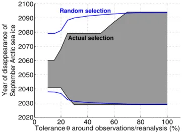
103km2decade−1) and the 1979–2010 reanalysed annual mean sea ice volume (18.95±3.79×10³km3). Among these six models, in RCP8.5, the 5-yr smoothed SSIE drops be-low 1 million km2 for at least 5 consecutive years first in 2041 and last in 2068. If a random selection of 6 models was operated, then on average these lower and upper bounds for year of disappearance would be 2037 and 2096, respec-tively (Fig. 6). This shows the interest of a selection based on a sound physical basis. As expected, tighter ranges for the year of September Arctic sea ice disappearance are obtained for smaller values ofθ. For example, the interval reduces to [2041, 2060] (same models, without IPSL-CM5A-LR) for
θ=15 %. The value for θ should not be decreased further as to account for uncertainties in observations and reanaly-sis. In RCP4.5,∼50 % of all CMIP5 models are not ice-free by 2100 (Fig. 1a). We are therefore not able to fully quantify the initial uncertainty on the year of disappearance of sum-mer Arctic sea ice because a limited number of CMIP5
mod-0 20 40 60 80 100
2020 2030 2040 2050 2060 2070 2080 2090 2100
Tolerance θ around observations/reanalysis (%) Year of disappearance of September Arctic sea ice
Actual selection Random selection
Fig. 6.Range of simulated years of disappearance of September Arctic sea ice, for RCP8.5. We define the year of disappearance of September Arctic sea ice as the first year during which the 5-yr smoothed September sea ice extent drops below 1 million km2 for more than 5 yr. A selection of models is applied following the methods defined in Sect. 3.4 for each toleranceθ around observa-tions/reanalysis. The black lines show the earliest and latest years of disappearance for the selected models as a function ofθ. The blue lines show the corresponding range that is obtained on average by selecting the same number of models randomly (10 000 draws) and ignoring the two models that are not ice-free by 2100 for which we do not have the year of summer Arctic sea ice disappearance.
els provide sea ice outputs after 2100. Withθ=15 %, the 5-yr smoothed SSIE drops below 1 million km2for at least 5 consecutive years in 2040 for the earliest selected model. Only one of the selected models is not ice-free by 2100 but it drops permanently below 2 million km2in 2080, which is an early timing compared to the other CMIP5 models that are not ice-free in 2100 (Fig. 1a).
4 Discussion
Still, we have reproduced the selection procedure described in Sect. 3.4 over the 1979–1995 period. 10 models were se-lected forθ=20 %. The mean bias of these 10 models com-pared to the observed 1996–2011 SSIE is 0.47×10⁶km2, and the mean bias of the 19 other, non-selected models is 1.74×10⁶km2. This example does not fully validate the hy-pothesis that a model performance is constant over time, but partly supports it.
Our selection is based on relationships between the base-line sea ice state and the year at which SSIE crosses a given threshold. Our analysis suggests that CMIP5 models tend to reach a given summer sea ice extent earlier when (1) they have smaller initial September sea ice extent , (2) the ampli-tude of their climatological cycle of sea ice extent is larger, (3) they have a smaller ice volume in the annual mean, (4) the extent of thin (<0.5 m) ice is larger in September, and (5) they lose ice at higher rates now. These results can, in addi-tion, be interpreted in light of simple physical mechanisms, resp. (1 and 3) models with a larger initial volume of ice need more energy, and thus time, to melt ice and reach a given ex-tent, (2) the seasonal cycle of sea ice extent is a proxy for the model sensitivity to the seasonal cycle of incoming so-lar radiation, (4) the ice is more susceptible to melt away in areas where it is thin, and (5) the most sensitive models now are likely to reach ice-free conditions earlier under fu-ture warming. It is also important to stress that these criteria are not fully independent. For example, the amplitude of the 1979–2010 mean seasonal cycle of sea ice extent correlates significantly (p <0.001) at 0.67 with the 1979–2010 mean September thin ice extent in the CMIP5 models.
As a final comment, we would like to discuss another pos-sible option aimed at reducing the spread in summer Arc-tic sea ice projections. Instead of applying a model selec-tion, one could consider retaining a linear combination of the models, for example a multi-model mean or a weighted av-erage of the different models. The multi-model mean would actually be selected at the 20 % tolerance level. As long as the CMIP5 models are not at (near) ice-free conditions, the CMIP5 model distribution is approximately Gaussian and symmetric (e.g. Fig. 2), two important properties that make the multi-model mean very informative. However, because the system is characterized by a highly nonlinear behaviour at low SSIE, and because the SSIE is by definition bounded by 0, the CMIP5 model distribution loses these two impor-tant properties when low SSIEs are reached. Consequently, the multi-model mean is no longer a good representative of the distribution since it results from an average of models in highly different states. A good illustration is given in Fig. 3: the U-shape present in each individual model is much more flat and less intense in the multi-model mean, simply be-cause it results from an average of all models at identical times; in other words, the diverse behaviours in each individ-ual CMIP5 model are much less visible in the multi-model mean.
5 Conclusions
The 21st century projections of summer Arctic sea ice are now available from the most recent effort of coupled model intermodel comparison, CMIP5. Here we consider 29 models available to date, starting from from the principle that none of the available CMIP5 models should be dismissed prior to the analysis (e.g. Arzel et al., 2006). Noticing a consider-able spread in the summer sea ice simulations over the 21st century, we raise the question of model selection as an op-portunity to reduce these uncertainties. In a first step, we find that the CMIP5 projected changes in September sea ice ex-tent (SSIE) with respect to their own 1979–2010 climatology are linked in a complicated manner to the 1979–2010 char-acteristics of their sea ice cover, owing to an acceleration of the trends (and thus larger changes) in SSIE, which occurs at different times during the 21st century, but at a mean SSIE of ∼2–4 million km2. Nonetheless, the year at which SSIE drops below a certain value correlates well with the 1979– 2010 sea ice properties. This supports the idea that a reduc-tion of spread through model selecreduc-tion is still possible.
adequate criteria for evaluation is challenging given that the sea ice dynamics operate on a very large spectrum both in the time and spatial domains (Rampal et al., 2009).
Our results are valid in the context of climate projections at the century time scale, and an equivalent intermodel study at shorter time scales, assessing for example the potential of ocean-sea ice initialization onto the simulated SSIE variabil-ity, is still lacking to the best of our knowledge. We have shown that it is possible to constrain the date of possible disappearance of summer Arctic sea ice as simulated by the CMIP5 models with a selection based on sea ice extent and volume characteristics. As for sea ice projections in gen-eral, the results are first and foremost scenario-dependent. For the medium scenario RCP4.5 and with a tolerance of 15 % around reference values, we reduce the uncertainty as to when the Arctic could become ice-free in summer from [2032, 2100+] to [2040, 2100+] (2100+=sometime after 2100). Only one of the selected model does not reach ice-free conditions in 2100 but it remains under 2 million km2 from 2080 onwards, which is not the case for the majority of models that are not ice-free by 2100 (Fig. 1a). With RCP8.5, the uncertainty in the year of summer Arctic sea ice disap-pearance reduces from [2029, 2100+]to [2041, 2060] after model selection. This represents a significant improvement compared to the initial uncertainty (Fig. 1b). In light of our results, and because there is always a possibility that some models simulate the 1979–2010 sea ice cover correctly for wrong reasons – for example through compensation of errors – we consider that reproducing a correct sea ice state over the recent decades is a necessary but not sufficient condition for models to reasonably anticipate future sea ice evolution. As we show, the 1979–2010 sea ice state indeed has a clear in-fluence on the variability and response of the summer Arctic sea ice cover.
Supplementary material related to this article is available online at: http://www.the-cryosphere.net/6/ 1383/2012/tc-6-1383-2012-supplement.zip.
Acknowledgements. We thank Editor J. Stroeve, reviewer D. Notz and an anonymous reviewer for insightful comments about the manuscript. We acknowledge the World Climate Research Programme’s Working Group on Coupled Modelling, which is responsible for CMIP, and we thank the climate modelling groups (listed in the supplement) for producing and making available their model output. For CMIP, the US Department of Energy’s Program for Climate Model Diagnosis and Intercomparison provides coordi-nating support and leads development of software infrastructure in partnership with the Global Organization for Earth System Science Portals. We thank P. Mathiot and M. Vancoppenolle for their helpful comments. FM is a F.R.S.-FNRS Research Fellow. HG is a F.R.S.-FNRS Senior Research Associate. This work was partly funded by the European Commissions 7th Framework Programme,
under Grant Agreement number 226520, COMBINE project (Comprehensive Modelling of the Earth System for Better Climate Prediction and Projection). It was also partly supported by the Belgian Science Federal Policy Office (BELSPO) and by the US Office of Naval Research through grant N00014-11-1-0550 (CMB).
Edited by: J. Stroeve
References
ACIA, Arctic Climate Impact Assessment (ACIA): Scientific Re-port, Cambridge University Press, Fairbanks, 2005.
AMAP. Snow, water, ice and permafrost in the Arctic (SWIPA): Cli-mate change and the cryosphere. Scientific report, Arctic Moni-toring and Assessment Programme (AMAP), Gaustadall´een 21, N-0349 Oslo, Norway (www.amap.no), 2011.
Armour, K. C., Bitz, C. M., Thompson, L., and Hunke, E. C.: Con-trols on Arctic Sea Ice from First-Year and Multiyear Ice Surviv-ability, J. Climate, 24, 2378–2390, 2011.
Arzel, O., Fichefet, T., and Goosse, H.: Sea ice evolution over the 20th and 21st centuries as simulated by current AOGCMs, Ocean Model., 12, 401–415, 2006.
Bitz, C.: Some aspects of uncertainty in predicting sea ice thinning, AGU Geophysical Monograph Series, edited by: deWeaver, E., Bitz, C. M., and Tremblay, B., 63–76, American Geophysical Union, 2008.
Bitz, C. M., Ridley, J., Holland, M., and Cattle, H.: Global cli-mate models and 20th and 21st century Arctic clicli-mate change, in: Arctic Climate Change: The ACSYS Decade and Beyond, chapter 11, edited by: Lemke, P. and Jacobi, H. W., Springer, Dordrecht and New York, 2012.
Bo´e, J., Hall, A., and Qu, X.: September sea-ice cover in the Arctic Ocean projected to vanish by 2100, Nat. Geosci., 2, 341–343, 2009.
Collins, M., Chandler, R. E., Cox, P. M., Huthnance, J. M., Rougier, J., and Stephenson, D. B.: Quantifying future climate change, Nature Clim. Change, 2, 403–409. doi:10.1038/nclimate1414, 2012.
Fetterer, F., Knowles, K., Meier, W., and Savoie, M.: Sea ice index, Electronic, available at: http://nsidc.org/data/seaice index/ (last access: July 2012), 2012.
Flato, G. M.: Sea-ice and its response to CO2forcing as simulated by global climate models, Clim. Dynam., 23, 229–241, 2004. Gent, P. R., Danabasoglu, G., Donner, L. J., Holland, M. M., Hunke,
E. C., Jayne, S. R., Lawrence, D. M., Neale, R. B., Rasch, P. J., Vertenstein, M., Worley, P. H., Yang, Z.-L., and Zhang, M.: The Community Climate System Model Version 4, J. Climate, 24, 4973–4991, doi:10.1175/2011JCLI4083.1, 2011.
Goosse, H., Arzel, O., Bitz, C. M., de Montety, A., and Van-coppenolle, M.: Increased variability of the Arctic summer ice extent in a warmer climate, Geophys. Res. Lett., 36, L23702, doi:10.1029/2009GL040546, 2009.
Gregory, J. M., Stott,. P. A., Cresswell, D. J., Rayner, N. A., Gor-don, C., and Sexton, D. M. H.: Recent and future changes in Arc-tic sea ice simulated by the HadCM3 AOGCM, Geophys. Res. Lett., 29, 2175, doi:10.1029/2001GL014575, 2002.
Wyman, B. L., Yin, J., and Zadeh, N.: The GFDL CM3 Coupled Climate Model: Characteristics of the Ocean and Sea Ice Simula-tions, J. Climate, 24, 3520–3544, doi:10.1175/2011JCLI3964.1, 2011.
Hazeleger, W., Severijns, C., Semmler, T., Stefanescu, S., Yang, S., Wang, X., Wyser, K., Dutra, E., Baldasano, J. M., Bintanja, R., Bougeault, P., Caballero, R., Ekman, A. M. L., Christensen, J. H., van den Hurk, B., Jimenez, P., Jones, C., Kallberg, P., Koenigk, T., McGrath, R., Miranda, P., Van Noije, T., Palmer, T., Parodi, J. A., Schmith, T., Selten, F., Storelvmo, T., Sterl, A., Tapamo, H., Vancoppenolle, M., Viterbo, P., and Will´en, U.: EC-Earth: A Seamless Earth-System Prediction Approach in Action, B. Am. Meteorol. Soc., 91, 1357–1363, doi:10.1175/2010BAMS2877.1, 2010.
Holland, M. M., Bitz, C. M., and Tremblay, B.: Future abrupt re-ductions in the summer Arctic sea ice, Geophys. Res. Lett., 33, L23503, doi:10.1029/2006GL028024, 2006.
Holland, M., Serreze, M. M., and Stroeve, J.: The sea ice mass bud-get of the Arctic and its future change as simulated by coupled climate models, Clim. Dynam., 34, 185–200, 2008.
Johns, T. C., Durman, C. F., Banks, H. T., Roberts, M. J., McLaren, A. J., Ridley, J. K., Senior, C. A., Williams, K. D., Jones, A., Rickard, G. J., Cusack, S., Ingram, W. J., Crucifix, M., Sexton, D. M. H., Joshi, M. M., Dong, B.-W., Spencer, H., Hill, R. S. R., Gregory, J. M., Keen, A. B., Pardaens, A. K., Lowe, J. A., Bodas-Salcedo, A., Stark, S., and Searl, Y.: The New Hadley Centre Cli-mate Model (HadGEM1): Evaluation of Coupled Simulations, J. Climate, 19, 1327–1353, doi:10.1175/JCLI3712.1, 2006. Jungclaus, J. H., Keenlyside, N., Botzet, M., Haak, H., Luo,
J.-J., Latif, M., Marotzke, J.-J., Mikolajewicz, U., and Roeckner, E.: Ocean Circulation and Tropical Variability in the Cou-pled Model ECHAM5/MPI-OM, J. Climate, 19, 3952–3972, doi:10.1175/JCLI3827.1, 2006.
Knutti, R., Furrer, R., Tebaldi, C., Cermak, J. and Meehl, G. : Chal-lenges in combining projections from multiple climate models, J. Climate, 23, 2739–2758, doi:10.1175/2009JCLI3361.1, 2010. Mahlstein, I., and Knutti, R.: Ocean heat transport as a cause for
model uncertainty in projected arctic warming, J. Climate, 24, 1451–1460, 2011.
Mahlstein, I. and Knutti, R.: September Arctic sea ice predicted to disappear for 2◦C global warming above present, J. Geophys. Res., 117, D06104, doi:10.1029/2011JD016709, 2012.
The HadGEM2 Development Team: Martin, G. M., Bellouin, N., Collins, W. J., Culverwell, I. D., Halloran, P. R., Hardiman, S. C., Hinton, T. J., Jones, C. D., McDonald, R. E., McLaren, A. J., O’Connor, F. M., Roberts, M. J., Rodriguez, J. M., Woodward, S., Best, M. J., Brooks, M. E., Brown, A. R., Butchart, N., Dear-den, C., Derbyshire, S. H., Dharssi, I., Doutriaux-Boucher, M., Edwards, J. M., Falloon, P. D., Gedney, N., Gray, L. J., Hewitt, H. T., Hobson, M., Huddleston, M. R., Hughes, J., Ineson, S., In-gram, W. J., James, P. M., Johns, T. C., Johnson, C. E., Jones, A., Jones, C. P., Joshi, M. M., Keen, A. B., Liddicoat, S., Lock, A. P., Maidens, A. V., Manners, J. C., Milton, S. F., Rae, J. G. L., Rid-ley, J. K., Sellar, A., Senior, C. A., Totterdell, I. J., Verhoef, A., Vidale, P. L., and Wiltshire, A.: The HadGEM2 family of Met Of-fice Unified Model climate configurations, Geosci. Model Dev., 4, 723–757, doi:10.5194/gmd-4-723-2011, 2011.
Maslanik, J. A., Fowler, C., Stroeve, J., Drobot, S., Zwally, J., Yi, D., and Emery, W.: A younger, thinner Arctic ice cover:
in-creased potential for rapid, extensive sea-ice loss, Geophys. Res. Lett., 34, L24501, doi:10.1029/2007GL032043, 2007.
Maslowski, W., Kinney, J. C., Higgins, M., and Roberts, A.: The future of arctic sea ice, Annu. Rev. Earth Pl. Sc., 40, 625–654, 2012.
Moss, R. H., Edmonds, J. A., Hibbard, K. A., Manning, M. R., Rose, S. K., van Vuuren, D. P., Carter, T. R., Emori, S., Kainuma, M., Kram, T., Meehl, G. A., Mitchell, J. F. B., Na-kicenovic, N., Riahi, K., Smith, S. J., Stouffer, R. J., Thom-son, A. M., Weyant, J. P., and Wilbanks, T. J.: The next gener-ation of scenarios for climate change research and assessment, Nature, 463, 747–756, doi:10.1038/nature08823, 2010. Notz, D. and Marotzke, J.: Observations reveal external driver
for arctic sea-ice retreat, Geophys. Res. Lett., 39, L08502, doi:10.1029/2012GL051094, 2012.
Parkinson, C. L., Vinnikov, K. Y., and Cavalieri, D. J.: Evaluation of the simulation of the annual cycle of Arctic and Antarctic sea ice coverages by 11 major global climate models, J. Geophys. Res., 111, C07012, doi:10.1029/2005JC003408, 2006.
Pavlova, T., Kattsov, V., and Govorkova, V.: Sea ice in CMIP5 mod-els: closer to reality?, Proc. MGO, 564, 7–18, 2011 (in Russian). Rampal, P., Weiss, J., Marsan, D., and Bourgoin, M.: Arctic sea ice velocity field: general circulation and turbulent-like fluctuations, J. Geophys. Res., 114, C10014, doi:10.1029/2008JC005227, 2009.
Rampal, P., Weiss, J., Dubois, C., and Campin, J.-M.: IPCC cli-mate models do not capture Arctic sea ice drift acceleration: con-sequences in terms of projected sea ice thinning and decline, J. Geophys. Res., 116, C00D07, doi:10.1029/2011JC007110, 2011.
Ridley, J., Lowe, J., Brierley, C., and Harris, G.: Uncertainty in the sensitivity of arctic sea ice to global warming in a per-turbed parameter climate model ensemble, Geophys. Res. Lett., 34, L19704, doi:10.1029/2007GL031209, 2007.
Rotstayn, L. D., Jeffrey, S. J., Collier, M. A., Dravitzki, S. M., Hirst, A. C., Syktus, J. I., and Wong, K. K.: Aerosol- and greenhouse gas-induced changes in summer rainfall and circulation in the Australasian region: a study using single-forcing climate simula-tions, Atmos. Chem. Phys., 12, 6377–6404, doi:10.5194/acp-12-6377-2012, 2012.
Sanderson, B. M. and Knutti, R.: On the interpretation of con-strained climate model ensembles, Geophys. Res. Lett., 39, L16708, doi:10.1029/2012GL052665, 2012.
Schweiger, A., Lindsay, R., Zhang, J., Steele, M., Stern, H., and Kwok, R.: Uncertainty in modeled arctic sea ice volume, J. Geophys. Res., 116, C00D06, doi:10.1029/2011JC007084, 2011.
Stroeve, J., Holland, M. M., Meier, W., Scambos, T., and Ser-reze, M.: Arctic sea ice decline: faster than forecast, Geophys. Res. Lett., 34, L09501, doi:10.1029/2007GL029703, 2007. Stroeve, J., Kattsov, V., Barrett, A. P., Serreze, M., Pavlova, T.,
Holland, M., and Meier, W.: Trends in arctic sea ice extent from CMIP5, CMIP3 and observations, Geophys. Res. Lett., 39, L16502, doi:10.1029/2012GL052676, 2012.
Voldoire, A., Sanchez-Gomez, E., Salas y M´elia, D., Decharme, B., Cassou, C., S´en´esi, S., Valcke, S., Beau, I., Alias, A., Cheval-lier, M., D´equ´e, M., Deshayes, J., Douville, H., Fernandez, E., Madec, G., Maisonnave, E., Moine, M.-P., Planton, S., Saint-Martin, D., Szopa, S., Tyteca, S., Alkama, R., Belamari, S., Braun, A., Coquart, L., and Chauvin, F.: The CNRM-CM5.1 global climate model: description and basic evaluation, Clim. Dynam., 1–31, doi:10.1007/s00382-011-1259-y, 2012.
Volodin, Dianskii, N. A. and Gusev, A. V.: Simulating Present-Day Climate with the INMCM4.0 Coupled Model of the Atmo-spheric and Oceanic General Circulations, Atmos. Ocean. Phys., 46, 414–431, doi:10.1134/S000143381004002X, 2010. Wang, M. and Overland, J. E.: A sea ice free summer
Arc-tic within 30 years?, Geophys. Res. Lett., 36, L07502, doi:10.1029/2009GL037820, 2009.
Wang, M. and Overland, J. E.: Summer arctic sea ice will be gone sooner or later – an update from CMIP5 models, Geophys. Res. Lett., 39, L18501, doi:10.1029/2012GL052868, 2012.
Watanabe, M., Suzuki, T., O’ishi, R., Komuro, Y., Watanabe, S., Emori, S., Takemura, T., Chikira, M., Ogura, T., Sekiguchi, M., Takata, K., Yamazaki, D., Yokohata, T., Nozawa, T., Hasumi, H., Tatebe, H., and Kimoto, M.: Improved Climate Simulation by MIROC5: Mean States, Variability, and Climate Sensitivity, J. Climate, 23, 6312–6335, doi:10.1175/2010JCLI3679.1, 2010.
Watanabe, S., Hajima, T., Sudo, K., Nagashima, T., Takemura, T., Okajima, H., Nozawa, T., Kawase, H., Abe, M., Yokohata, T., Ise, T., Sato, H., Kato, E., Takata, K., Emori, S., and Kawamiya, M.: MIROC-ESM 2010: model description and basic results of CMIP5-20c3m experiments, Geosci. Model Dev., 4, 845–872, doi:10.5194/gmd-4-845-2011, 2011.
Winton, M.: Do climate models underestimate the sensitivity of Northern Hemisphere sea ice cover?, J. Climate, 24, 3924–3934, doi:10.1175/2011JCLI4146.1, 2011.
Zhang, X.: Sensitivity of Arctic summer sea ice coverage to global warming forcing: toward reducing uncertainty in Arctic climate change projections, Tellus A, 62, 220–227, 2010.