Bluetongue Vector
Culicoides brevitarsis
in Australia
Joel K. Kelso, George J. Milne*
School of Computer Science and Software Engineering, University of Western Australia, Crawley, Western Australia, Australia
Abstract
Background:The spread of Bluetongue virus (BTV) among ruminants is caused by movement of infected host animals or by movement of infected Culicoides midges, the vector of BTV. Biologically plausible models of Culicoides dispersal are necessary for predicting the spread of BTV and are important for planning control and eradication strategies.
Methods:A spatially-explicit simulation model which captures the two underlying population mechanisms, population dynamics and movement, was developed using extensive data from a trapping program forC. brevitarsison the east coast of Australia. A realistic midge flight sub-model was developed and the annual incursion and population establishment ofC. brevitarsiswas simulated. Data from the literature was used to parameterise the model.
Results:The model was shown to reproduce the spread ofC. brevitarsissouthwards along the east Australian coastline in spring, from an endemic population to the north. Such incursions were shown to be reliant on wind-dispersal;Culicoides midge active flight on its own was not capable of achieving known rates of southern spread, nor was re-emergence of southern populations due to overwintering larvae. Data from midge trapping programmes were used to qualitatively validate the resulting simulation model.
Conclusions:The model described in this paper is intended to form the vector component of an extended model that will also include BTV transmission. A model of midge movement and population dynamics has been developed in sufficient detail such that the extended model may be used to evaluate the timing and extent of BTV outbreaks. This extended model could then be used as a platform for addressing the effectiveness of spatially targeted vaccination strategies or animal movement bans as BTV spread mitigation measures, or the impact of climate change on the risk and extent of outbreaks. These questions involving incursiveCulicoidesspread cannot be simply addressed with non-spatial models.
Citation:Kelso JK, Milne GJ (2014) A Spatial Simulation Model for the Dispersal of the Bluetongue VectorCulicoides brevitarsisin Australia. PLoS ONE 9(8): e104646. doi:10.1371/journal.pone.0104646
Editor:Lars Kaderali, Technische Universita¨t Dresden, Medical Faculty, Germany
ReceivedSeptember 8, 2013;AcceptedJuly 15, 2014;PublishedAugust 8, 2014
Copyright:ß2014 Kelso, Milne. This is an open-access article distributed under the terms of the Creative Commons Attribution License, which permits unrestricted use, distribution, and reproduction in any medium, provided the original author and source are credited.
Funding:Research was funded by Meat and Livestock Australia (project number B.AHE.0037). The funders had no role in study design, data collection and analysis, decision to publish, or preparation of the manuscript.
Competing Interests:The authors declare that no competing interest exist.
* Email: [email protected]
Introduction
The past decade has seen the development of increasingly detailed simulation models aimed at capturing the transmission dynamics of directly transmitted diseases, such as Foot and Mouth Disease and Classical Swine Fever in livestock [1–4] and human pandemic influenza [5–7]. Such models have been used to establish the effectiveness of intervention strategies and to develop containment and control strategies (e.g. for human pandemic influenza [5–7]) and eradication strategies (e.g. for Foot and Mouth Disease [1]).
The development and use of mathematical disease models of insect-vectored human diseases dates back over a century to the work by Ross on malaria transmission [8]. However, the development of data-rich simulation models for insect-vectored diseases has advanced more slowly, mainly due to the additional complexity inherent in representing the dynamics of both host and vector populations, and pathogen transmission between them. An additional layer of complexity is introduced if the goal is to model the spatial spread of a pathogen over a landscape since both vector
movement and habitat-dependent insect vector abundance potentially affect spatial disease spread. Faster moving vectors clearly have the potential to increase the rate of disease spread; but disease spread may also depend on the population density of vectors, since greater vector numbers mean greater transmission of pathogen between vectors and host as well as greater numbers of vectors moving to new locations. For example, high densities of mosquitos in particular locations are known to lead to disease transmission ‘hot spots’ and are often the focus of targeted control measures for mosquito vectored diseases [9]. Hence spatial vector population features need to be realistically modelled within a modelling environment if it is to be used to analyse the effectiveness of spatially targeted intervention strategies.
can change seasonally or from year-to-year in a way that depends on vector introduction and dispersal.
Our motivating example of an incursive vector population is the biting midge Culicoides brevitarsis which is present in northern and eastern Australia and is a vector for several viral livestock diseases, including Bluetongue, which is caused by Bluetongue Virus (BTV), and Akabane [10].C. brevitarsissurvival and activity is temperature dependent;C. brevitarsisis present throughout the year in northern areas of New South Wales (NSW), but is unable to survive the cold winter period in southern areas [11,12]. The spatial distribution of C. brevitarsis within NSW thus varies seasonally during the year, and from year to year, depending on spatiotemporal variation in temperature and wind, as midges are transported from northern areas into more southerly areas where they establish breeding populations in warmer months, and become locally extinct over winter. This Culicoides movement scenario is also reflective of past, well-documented incursions ofC. imicolacarrying BTV into the Balearic Islands (Spain) from North Africa [13], the probable wind dispersal of Culicoides between Greece, Turkey and Bulgaria [14] and what may occur if a new (to Australia) competent vector were to arrive from Indonesia, East Timor or Papua New Guinea and establish itself in Australia, see [15].
Incursive vector populations may be contrasted with endemic
populations. An endemic population is permanently established and a breeding cycle will be sustained without introduction of transported population, even if the population falls to very low levels. TheCulicoides obsoletusgroup BTV vectors are an endemic population in Northern Europe, which carried outbreaks of BTV in the summers of 2008 and 2009. In these outbreaks, once the warming created a vector population capable of sustaining BTV transmission, BTV spread was limited only by vector movement and not by temperature-dependent vector population dynamics.
The distinction between incursive and endemic vector popula-tions is very significant from a modelling perspective, as the endemic scenario allows the simplifying assumption that vector population distribution does not depend upon vector movement, and so can be treated as a static model input. In the incursive vector scenario, this assumption is invalid, and both vector population dynamics and dispersal need to be modelled in tandem.
A simulation modelling methodology which permits spatially-explicit modelling of wind and flight movement of C. brevitarsis
dispersal, together with its habitat and climate dependent population dynamics, is presented. The particular incursive scenario in coastal NSW is used to illustrate the development and application of the modelling methodology. Extensive trapping over the past four decades has resulted in high quality data which reports the arrival time ofC. brevitarsisas it spreads southwards along the NSW coastal plain [11,16–20]. These data permit the simulated midge incursions produced by the model to be validated by comparison with the field-derived datasets, and these results are presented. For other Culicoides species their specific habitat- and temperature-dependent characteristics would need to be modelled and the simulation model presented here re-parameterised. This is a region without a resident population of competent BTV midge vectors. C. brevitarsis is a competent tropical midge species common to northern Australia but populations of this midge cannot be sustained in most of NSW due to low winter temperatures. Annual incursions occur from endemic areas to the north, as the temperature increases in spring. This southward incursion scenario is significant in that it may act as a BTV conduit, allowing the virus to spread from endemic regions to the
north to vulnerable, disease-free sheep-rearing areas in south-east Australia.
1.1 Background
Various species of Culicoides biting midges are present throughout the world with the exception of Antarctica and New Zealand. Where they are present,Culicoidescan act as vectors of BTV, Akabane virus (and other viruses of the Orthobunyviridea family) and African Horse Sickness [10]. Competent Culicoides
species are those capable of viral transmission, with susceptible female midges becoming infected following blood-feeding by biting an infectious ruminant host animal. As trans-ovarial BTV transmission (where infected females transfer the virus to their offspring) is unknown in Culicoides, onward animal infection occurs when infectious midges subsequently feed a second time on susceptible, uninfected animals.
Bluetongue is a significant disease from an animal health and economic perspective world-wide. In cattle, BTV infection is generally asymptomatic but its presence limits export to certain markets. In sheep, BTV infection is symptomatic and induces significant mortality rates, with 30% mortality rates recorded for epidemics in Spain, for example [21]. BTV is endemic in northern Australia but disease free status exists in the southern sheep rearing regions. The vectors considered to be most important in Australia areC. fulvus, which is an efficient vector but is restricted to areas with high summer rainfall and does not occur in the drier sheep-rearing areas of Australia; C. wadai, which is also an efficient vector that probably spread from Indonesia in the 1970s and has extended its range from an initial area near Darwin into Western Australia, Queensland, and New South Wales; andC. brevitarsis, which is a competent but inefficient vector for the BTV strains present in Australia but is more abundant thanC. fulvusorC. wadai[10].C. brevitarsis is a midge species that relies on cattle dung for ovipositioning (i.e. egg laying) and is endemic in northern Australia, but not in the sheep-rearing areas of Southern Australia. In an Australian setting, the future spread of BTV may be impacted by changes to weather patterns [22], the incursion of new competent insect vectors from Asia (i.e. new species of
Culicoidesmidge carried by the wind) [15] or the incursion of new serotypes of BTV (which might have different competence characteristics) from Asia via midge dispersal. The risk to both commercial export markets and animal health caused by high mortality rates in sheep populations makes Bluetongue a disease of significance.
The spread and establishment of BTV in northern Europe [23] demonstrated a previously unforeseen ability of BTV to become endemic in cooler climates. This has resulted in increased research activities in virus transmission, on detailed reporting of these outbreaks [24,25] and in initiation of modelling studies, for example [26–28].
Culidoidesmidges are known to be dispersed by the wind, often over large distances over water and lesser distances over land. Studies have found long-range spread across the Mediterranean Sea from North Africa to Spain [13], and from Indonesia and Papua New Guinea to Australia [15,29], for example. A number of studies have examined long-distance movement of Culicoides
animals with the same BTV serotype and the only route of BTV spread could have been via transportation by the midge vector (i.e., no animal movements from possible source locations to the arrival location of the virus) then a likely path of midge movement is detected. Data from such studies indicate distances of greater than 100 km over water (and lesser distances over land) are possible, indicating that any modelling of midge or BT spread should include a wind-driver midge dispersal component.
C. brevitarsisoccupies a particular environmental niche in that it lays its eggs solely in cattle dung [30]. Like other insect vectors, only the female midge bites the mammal host, as it requires blood meals to aid egg development. The population dynamics of both mosquitoes and midges are highly dependent on weather conditions, particularly on temperature. Each species has an optimal temperature range where flying, feeding and mating activity is at its maximum, which also minimizes the egg development period following mating. Temperature also affects the extrinsic incubation period, the time from insect infection (by biting an infected host animal) to becoming infectious itself and thus capable of virus transmission to a new, possibly uninfected, host.
Methods
2.1 Modelling Landscape via Discrete Cells
The aim of the simulation model is to predict the spread and population establishment, growth and die-out ofCulicoidesmidges over the landscape through time. This is achieved by representing thestateof the landscape – that is, landscape information which is relevant to midge spread and population dynamics including habitat-dependent features – in a data structure. A simulation algorithm is then used to capture the physical processes which contribute to insect spread using computer software which updates the data structure to reflect the physical system changes, from one simulation time step to the next.
The landscape is represented by dividing it into a regular array of spatial cells of similar area, depending on the resolution required. In this study a graticule (i.e. a grid based on lines of latitude and longitude) with 0.05 degree spacing have been used, giving cells that are approximately square with 5 km sides, each with an area of approximately 2500 hectares. The 5 km cell spacing is small enough to represent the spatial heterogeneity in climate (such as altitude dependent temperature) and to represent midge dispersal (as discussed in subsection 2.3 below), while at the same time being large enough to make simulation time tractable. Single cells are the finest level of spatial detail captured by the simulation model and cells are considered to have uniform characteristics throughout their area. Each cell has a centroid location (latitude/longitude co-ordinates and altitude) and addi-tional information which captures the state of the landscape represented by the cell. A summary of the data contained in each landscape cell is given below; further details are given in subsequent sections where the simulation processes that update each cell state are described.
Geographical data includes latitude, longitude, altitude and area. The relative location of cells determines distance and direction between neighbouring cells, which influences the spatial dispersal of midges by prevailing wind conditions.
Weather dataincludes daily mean temperature, wind speed, and wind direction. Weather data enters the model as an input data time series. Temperature, including lower temperatures due to altitude, influences the model in multiple ways including the insect reproduction rate, survivability and biting and movement activity. Wind drives vector dispersal.
Vector habitat data.ForC. brevitarsisthe key characteristic of the habitat is whether cattle are present or not within each cell, as cattle are necessary for ovipositioning, as C. brevitarsisonly lay eggs in cattle dung [30], and also for females to blood feed (necessary for egg development within the female).
Vector population data.Two population density variables, for the adult and immature stages (egg, larvae, and pupae collectively), represent theC. brevitarsis population state of each cell. Unlike geographic, weather or vector habitat data, the vector population data represented in the model are endogenous state variables which both influence, and are influenced by the simulation dynamics.
Cell data fields are given in Text S1, Tables S1.1 and S1.2.
Simulation methodology. As the landscape is approximated by a discrete array of cells, the time course of midge spread over the landscape is characterized by local processes that occur within individual cells and processes that model the movement of insects between cells. Time is also treated discretely; state changes (called transitions) occur only at the discrete time points when one time period changes to the next, and the state variables remain fixed for the duration of each period. The dynamic behaviour of each discrete landscape cell is modelled by a correspondingautomaton, a mathematical device which captures the changing state of a cell based on its current state and the state of neighbouring cells with which it interacts [31]. An automaton consists of state information together with a transition function which models how the state changes through time. This is anautomata theoreticapproach to modelling the inherently continuous behaviour of a complex system; which in this application involves the location of the midges in discrete time and space.
This conceptual automata theoretic model is implemented in software and the dynamics of the midge population (involving population growth and decline) together with vector movement is realized by discrete event simulation [32]. The landscape cell automata state data and the transition functions are used by the
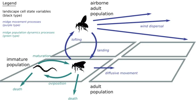
simulation algorithmto update the state of each automaton at an appropriate discrete time step, capturing the dynamic behaviour of the physical system being modelled. An outline of the simulation algorithm is given in Text S1. The specific dynamic processes that determineCulicoidesspread, namely the changing weather, insect population dynamics, and insect movement between cells may be treated as sub-models which are combined together to produce the overall simulation system. These sub-models are depicted sche-matically in Figure 1 where 4 discrete cells are pictured for illustrative purposes, and are described in detail in subsequent sections.
Model timelines. The main simulation algorithm operates by updating theCulicoidespopulation within each landscape cell in a daily cycle.Culicoidespopulation dynamics and self-propelled midge movement are calculated on a daily basis, while wind-driven midge movement is calculated on a finer 3-hourly cycle, with 8 such cycles occurring within each daily cycle.
2.2 Weather
The distribution of vectors over the landscape and changes in vector density over time is influenced by the weather, specifically temperature and wind speed and direction. This variability is taken into account through the spatial weather model.
Temperature Data. Daily maximum and minimum tem-peratures were obtained from the Australian Bureau of Meteorol-ogy for an approximately 5 km square cell grid covering the land area of Australia (including NSW), for the period 1980–2000. This data set is based on automatic weather station (AWS) and topographic (altitude) data and uses a Barnes successive correction technique to interpolate temperature at each grid point [33,34]. Mean daily temperatures, which are well approximated by the averaged daily maxima and minima, were used as inputs for temperature dependent population dynamics sub-model (de-scribed below). Temperature also influences midge flight behav-iour with research indicating thatC. brevitarsismidges take flight when the temperature is 18uC or greater [20]. Days when the mean daily temperature was greater than or equal to 18uC were regarded as ‘‘midge activity’’ days, a concept used by the midge dispersal sub-model (described below).
Wind Data. Data from the Australian Bureau of Meteorology for all automatic weather stations (AWS) in NSW for the 1980– 2000 period at three-hourly resolution was obtained. Data from 133 AWS were used – a map showing the distribution of weather stations is included in Text S1, Figure S1.2. This wind speed and wind direction data (measured at 10 m above ground) was used in the midge dispersal sub-model. Each landscape cell used wind data from the nearest AWS. Intermittent gaps in AWS data were overcome by taking data from the nearest AWS that had valid data for the gap period.
2.3CulicoidesPopulation Dynamics
When significant cattle numbers are present, the key determin-ing factor in C. brevitarsispopulation density is the climate. In areas where the climate is favourable, specificCulicoidesspecies
may be present and active all year round [35]. In other areas, the
Culicoidespopulation, and its activity, may become low during winter as a result of lower temperatures. In still other areas, the climate may support incursions ofCulicoidespopulations during summer, but extended cold winters may render them locally extinct; this is the case in New South Wales, Australia which is the scenario under consideration here [11,35].
The characteristics that constitute vector habit vary between
Culicoidesspecies, however cattle are necessary forC. brevitarsis. The rate at whichC. brevitarsis populations can grow and the maximum density attainable depends critically on the presence of cattle and the availability of dung for ovipositioning (i.e. egg laying) [30], in addition to the temperature. In areas of the landscape being modelled where cattle are absent, such as in National Parks and urban areas, noC. brevitarsispopulation can be sustained and any insects dispersed into these areas fail to establish a breeding population. Any transported midges that come to rest in these cells are assumed to die without having any further effect on the simulation. Note that these cells can carry an airborne population, so these areas do not form a complete barrier to midge spread.
When supplied with an initial insect population and daily temperature time series, the population dynamics sub-model described below generates adult and immature stages of the midge population as a time series for each landscape cell. Temperature-dependent midge population dynamics generated by the simula-tion sub-model are presented below, in the subsecsimula-tion entitled
Climate scenarios.
Each landscape cell may be in one of threeinsect population states:
a) Active; indicating that midges are present in the cell and are actively flying (necessary for feeding and mating) and that the breeding cycle is on-going. In cold conditions, breeding and development rates may slow to the point where they are exceeded by the adult death rate, in which case the population will fall, and may become inactive.
Figure 1. Schematic overview of the simulation model components.The dynamic state variables (population densities) are shown in black type. The processes midge movement modelling midge movement are shown in purple; processes modelling midge population dynamics are shown in green.
b) Inactive; indicating that adult population numbers are very low. If temperatures subsequently rise, a cell in the inactive state may become active as immatureCulicoidesemerge from their pupal stage. Alternatively, sufficiently cold and sustained conditions may kill or render unviable all adult and immature
Culicoides, making the insect population extinct within that cell.
c) Extinct; indicating that no viable Culicoides are present in any life stage (adult, larvae, or pupae). As a result, improving changes in weather or habitat conditions will not cause any change in the cell population state. However, if new midges are transported into the cell and conditions are favourable, the cell state may then transition into an active state. It should be noted that while the active state can be detected from midge trapping programs, the inactive and extinct states cannot be distinguished in this way. The extinct population state may be inferred retrospectively from the lack of trapped midges once the temperature has risen to the point where any active population would be detected.
These states and the possible transitions between them are illustrated in Figure 2.
Cells in the active and inactive states have two additional numeric attributes representing the population density of the adult female (pa) and immature (pi)Culicoides(taken to include all
pre-adult stages) in the landscape cell. We did not attempt to estimate absolute midge population density. Instead, we assume that at any given time the numerical ‘‘size’’ of the simulated midge population is some proportion of the maximum population in the cell. We have set the population scale by defining the (maximum) carrying capacity of the immature population of a cell to have an arbitrary numerical value of 100. Other midge density values that appear in the model are interpreted as relative to this value.
It was assumed that population density evolved according to a logistic population model [36,37]. This is a standard model of population dynamics that exhibits a maximum growth rate when unconstrained by resources, but where the growth rate decreases with increasing population density, representing increasing com-petition for some finite resource required for growth. In the model three on-going processes modify the density of the adult and immature populations: the oviposition of eggs by adult females; the maturation of eggs into adults; and the death of both adults and immatures. The rate at which these processes occur is temperature dependent. In the process descriptions below, rates are given for key temperatures, and the dependency of the rate on temperature were modelled as piecewise linear functions of temperature (i.e. rates were interpolated linearly between key temperature values).
One particular temperature plays a role in several processes – we refer to this as thelow temperature activity parameter(LTAP). The LTAP value of 7uC was determined using data distinguishing C.
brevitarsisclimatic zones, as described below in Section 2.4 (in the subsection entitledPopulation initialisation).
1.Oviposition. Adult femaleCulicoidesperform a cycle of blood feeding followed by oviposition (egg-laying). The rate at which adult midges lay eggs (denoted by parameter value b) in Figure 3 depends on temperature. We assumed (from [12,38,39]) that a maximum oviposition rate of 3.9 viable eggs per adult female per day at temperatures of 25uC and above, a rate of 1.1 at a temperature of 18uC, and a rate of zero at the LTAP temperature. These rates were derived by dividing the fecundity (number of eggs layed per oviposition) by the mean gonotrophic period, and further dividing by two (since half of the eggs laid are destined to emerge as males and are not included in our adult population density measure which represents only females [12]).C. brevitarsisfecundity averages 31.3 eggs per oviposition [38]. Data on the gonotrophic period and its temperature dependence inC. brevitarsisis sparse; we assumed that the gonotropic cycle length varies from a minimum of 4 days to 14 days based on studies of C. sonorensis [39]. The temperature point of 25uC giving the maximum oviposition rate corresponds to the temperature of the shortest gonotrophic period reported in [39], while the 18uC value corresponds the minimum temperature at which C.
brevitarsis have been observed to fly (and thus to oviposit). Rather than assume that oviposition ceases exactly at 18uC, we assume that it decreases gradually to zero at the LTAP value, at 7uC.
1. It was assumed that there is a limiting population level for immature midges, which in the case of C. brevitarsis is determined by the availability of cattle dung, which provides habitat and nutrition for immature stages; density limited
Culicoides larval development is reported in [40]. It was assumed that the number of viable eggs laid decreases with increasing immature population density, since eggs laid in already crowded dung will fail to develop due a lack of available nutrition. An alternative method of modelling the immature population density limit would be to increase the immature death rate in crowded conditions; however it is not obvious that this would be a more accurate assumption, since it might be the case that later-laid eggs do not significantly decrease the mortality of more developed larvae (or pupae) originating from earlier laid eggs. As explained previously, an arbitrary value of 100 was chosen for the limiting immature population density, and all other absolute population quantities are relative to this value.
2.Maturation. Culicoides larvae hatch from eggs and develop into pupae, from which they emerge as adults. Based on experimental data forC. brevitarsis[12], the maturation rate (denotedmin Figure 3) was assumed to be 11 days at 36uC, 37 days at 18uC, and zero at the LTAP temperature.
3.Death. Adult and immatureCulicoideswere assumed to die at a given temperature dependant rate. There are no published estimates of adult lifespan forC. brevitarsis: based on data on
C. sonorensis[39], it was assumed that the mean lifespan varied from 4 days at 25uC, to 14 days at 12uC and below.
Estimates of immature midge lifespan and dependence of lifespan on temperature were based on experimental data where cattle dung that had been exposed to oviposition was collected and subjected to different temperature treatments
Figure 2. Landscape cell vector population state.Landscape cell population states are pictured as boxes; arrows indicate transitions between states with arrows labelled according to the events or conditions that trigger the state transition.
[12]. Based on total numbers of adults emerging from dung held at 17uC for 28 and 42 days, it was assumed that immature
C. brevitarsishad a mean lifespan of 30.5 days. Note that the immature ‘‘lifespan’’ is the mean time when an immatureC. brevitarsis (egg, larva, or pupa) dies, given that it has not matured into an adult. While total numbers of emerging midges increased with increasing temperature above 17uC (up to 25uC), this might be due to an increased maturation rate (with moreC. brevitarsismaturing into adults rather than dying in immature stages) rather than increased lifespan. We therefore adopted a simpler model with constant immature lifespan above 17uC. Similarly, the experimental data showed that mortality might increase at lower temperatures; however the numbers of emerging midges were too low to allow quantitative analysis of lower temperature lifespan. Conse-quently we assumed that immature lifespan decreased to 1 day at the LTAP value.
We note that the use of a single temperature at which oviposition and maturation ceases is a simplification of the actual temperature dependencies; however this model was able to adequately reproduce the observed climatic zones. A more sophisticated model could be substituted if additionalC. brevitarsis
data becomes available.
The relationship between these processes is illustrated in Figure 3. The population dynamics model variables and param-eters, along with parameter values and supporting references are summarised in Tables S1.3 and S1.4 in Text S1.
The vector population dynamics sub-model cell can be described as a variant of the classic logistic population dynamics model [36], using two ordinary differential equations (ODE) as follows.
dpa
dt ~mpi{dapa
dpi dt ~b(1{
pi pimax
)pa{dipi{mpi
The top equation captures the dynamics of the adult midge populationpain terms of the maturation ratem(of immaturespi
into adults) minus those adults which diedapa. The lower equation
models the dynamics of the immature midge stages in terms of the birth rateb(following oviposition by adult females) which reduces to zero when the habitat capacity of that cell reaches a maximum
pimax. The size of the immature population is depleted by the
immature death ratedipiand by the maturation of immatures into
adultsm pi. Note that the parametersb,di,da, andmare functions
of temperature, as described previously.
The implemented model differs from the ODE system described above in three ways.
1. The model is a discrete-time difference equation with one-day time steps. In other words, for each cell, the temperature-depended rate parameters are calculated using the temperature for that day; the numbers of ovipositions, maturations, and deaths are calculated using the rate parameters and current populations, assuming the rate maintains a fixed value during the day; and the immature and adult population numbers are then updated accordingly. This process is fully deterministic. 2. When mature and immature populations (a) fall below levels
designated minima ei and ea, respectively and (b) are
decreasing, it is assumed that they become zero. Without this feature, vector populations would never become extinct regardless of how close to zero they become, which is unrealistic. Since we did not attempted to estimate absolute midge populations, values of 0.001 and 0.0005 were chosen as small but arbitrary values foreiandearespectively. A sensitivity
analysis showed that,eiandeacould vary over two orders of
magnitude without changing the outcome of the population sub-model calibration process (see Section 2.4 below). The stipulation that small populations only become extinct if they are decreasing has the consequence that when very small midge populations (less thanea) are dispersed into an empty
cell, they do not automatically become extinct. Rather, if the temperature in the destination cell is conducive to population growth, a population will become established; otherwise the dispersed population will become extinct.
3. The immatureCulicoidespopulation density limit factor is not (12pi/pimax) but max (0,12pi/pimax), i.e. when pi.pimax the
oviposition rate is zero and does not become negative.
Significant temperatures. As a result of temperature dependencies, the behaviour of the population dynamics sub-model has two important temperature regimes.
At temperatures above 17uC, adult activity is high, giving a high oviposition rate. Although adult mortality increases with temper-ature, the oviposition rate also increases meaning that fecundity does not decrease with increasing temperature. In addition, the immature maturation period is short and most immature midges successfully emerge and do not die in the immature state [12]. In this temperature regime, the population grows until the oviposition rate is limited by the immature population densitypi/pimax. This is
theactivestate referred to in Figure 2.
At temperatures below 17uC adult activity is low, giving a low oviposition rate. Furthermore the immature maturation period is long, becoming comparable to the immature lifespan, and immature mortality becomes significant. With fewer midges emerging and a slow rate of oviposition the immature and adult populations decline and eventually become extinct. Note that due to the relatively long immature lifespan, the immature population may take several months to become extinct after the initial adult population collapses. The period between the adult and immature populations becoming zero is the inactive population state referred to in Figure 2.
In addition to these processes, insect dispersal also alters cell population states, with adults being moved out of some cells and into others; see Section 2.3 below.
Climate scenarios. The vector population sub-model is capable of representing Culicoides population dynamics having
three distinct climatically driven patterns, each of which has different consequences for BTV incursion and transmission. Simulations of these climatic scenarios for C. brevitarsis are presented in Figure 4, following seeding of midges from day zero.
1. Regions in which the climate allowsC. brevitarsispopulations to exist actively throughout the year. In these areas the midge population remains in the high-temperature regime (above 17uC), although the population may seasonally fluctuate as the activity and breeding rate varies with mean daily temperature [18,41,42]. This population dynamics scenario is illustrated in Figures 4A and 4B, which show simulation output of population time series for areas where the mean temperature varies seasonally from 25–27uC and 16–26uC respectively, following initial ‘‘seeding’’ of midges from time zero.
2. Regions in which the midge population undergoes large fluctuations but does not become extinct. In these areas the population is in the high-temperature regime in spring, summer and autumn but falls into the low-temperature regime for a period during winter. There may be times of the year in which adult C. brevitarsis population becomes very low (and may also be incapable of transmitting BTV) but the C. brevitarsis population recovers each year without external introduction when the temperature rises and surviving immature stages emerge and re-start the breeding cycle [12]. This scenario is illustrated in Figure 4C, which shows simulation output for an area where the mean temperature seasonally varies from 13–21uC.
3. Regions in whichC. brevitarsiscan only survive seasonally. In these areas incursions may result in a population becoming established due to higher summer temperatures, but in winter the population reverts to the low-temperature regime for such a duration that both the adult and immature populations become extinct [11]. This is illustrated in Figure 4D, which has conditions two degrees cooler than Figure 4C. Note that the fact that the number of C. brevitarsis found by trapping programs falls to zero does not show population extinction by itself. The inference that the population does become locally extinct is made from fact that when the temperature rises the following spring, trapped midge numbers do not rise with the rising temperatures as they do in warmer northern areas where they do clearly overwinter. Instead, midges are not detected until a time delay has passed, with the delay being approximately proportional to the distance fromC. brevitarsis
endemic areas [43].
The model ofCulicoidespopulation dynamics described here is based onC. brevitarsisbut model parameterisation allows for the population dynamics of other Culicoides midge species to be represented.
2.4CulicoidesMidge Movement
Two types of insect movement can occur,wind-blown dispersal
and diffusive spreadvia active flight. Each cell centroid location (latitude/longitude co-ordinates and altitude) and cell size can be adjusted to suit the scale of the simulation, as a trade-off between spatial resolution and computational efficiency. The relative location of cell centroids determines the distance and direction between neighbouring cells, with between-cell dispersal of midges depending upon the distance between cells and prevailing wind direction and speed.
Diffusive spread. Culicoidesmidges are significantly smaller than most mosquito species and do not exhibit self-propelled long range movements. In the absence of wind or other directional
stimuli, they can be assumed to move according to a random walk process with typical movement ranges up to 100 m per day. Such behaviour has been observed by trap-mark-release-trap field experiments which showed that typical daily (or nightly) flight ranges of midges are mostly on the order of a few hundred meters [44,45]. The collective movement behaviour of a large number of insects executing a random walk can be modelled as a diffusion process [46,47]. When implemented in our cell-based spatially discrete simulator, this process moves a small proportion of midges to neighbouring cells during each simulation cycle. The same trap-mark-release-trap experiment cited above showed that at least a small percentage of midges travelled at least 4 km in 24 hours, so it is expected that a small percentage of midges will move to a neighbouring 5 km cell in each 24 hour simulation cycle, and our representation of self-propelled midge movement as a diffusion process captures this phenomena.
In a cellular implementation of a diffusion model, the quantity of particles (in this case midges) moving between cells depends upon the population density of the cells, the cell size, and a diffusion coefficient which characterises the movement of the diffusing species. Two studies report diffusion coefficients for
Culicoides species: 60.1 m2/s for C. impunctatus [47,48] and 12.96 m2/s forC. variipennis[45,49]; there does not appear to be any similar quantified dispersal data for C. brevitarsis. The C. variipennisvalue was adopted, since the methodology by which it was derived is described in much greater detail compared to the
impunctatus value. A sensitivity analysis was performed which examined alternative diffusion coefficients ranging from 6.5 m2/s to 120 m2/s (see Text S1). Results of idealised proof-of-concept simulations demonstrating the effect of the diffusive midge transport model are shown in Text S1, Figure S1.1.
As indicated by experimental data on C.brevitarsisbehaviour, diffusive dispersal was assumed to occur only on days when the mean temperature was 18uC or greater. Further details of the implementation of the diffusive movement model can be found in Text S1.
Wind-borne dispersal. For the purposes of wind dispersal, each 1-day simulation cycle was also broken in to 3-hour wind sub-cycles. This fine grain time period is required as the flying behaviour of most midge species differs between dawn and dusk, and other times of the day.Culicoidesare active (that is fly, feed, mate and egg-lay) when winds are no stronger than 8 km/h. If winds are stronger they generally stay on the ground attached to plants [20].C. brevitarsisare known to be most active immediately before and after dusk and active to a lesser extend just before dawn. Once flying they may be lofted above their usual 3–4 meter flying height by thermals or by topography-induced wind turbulence, allowing them to reach higher altitudes with possibly stronger winds [13,15].
Wind-driven midge transport was modelled representing two midge sub-populations in each cell, a ‘‘grounded’’ and a ‘‘flying’’ population. It was assumed that three processes occurred in each landscape cell during each 3-hour period:
midges becoming airborne in each favourable 3-hour period). There is unfortunately no existing data to inform this model parameter. A sensitivity analysis was conducted to assess the sensitivity of the overall spread dynamics to this parameter (details can be found in Text S1, Table S1.6).
2.Wind transport. Midges currently airborne were transported into a number of cells in a ‘‘footprint’’ downwind of the source cell. It was assumed that midges would be carried at the speed of the wind. The AWS wind data source used recorded winds at a standard height 10 m above ground. We considered that midges may be transported by winds which may be faster or slower than 10 m winds, since wind speeds generally increase with altitude due to the surface wind gradient. We assumed that the maximum midge transport speed was some multipli-cative factor of the recorded 10 m wind speed (as midges may be carried at higher altitudes), and calibrated this multiplier to achieve the best fit to observedC. brevitarsis arrival times at trapping sites in NSW in 1991/1992 [11]. This calibration process is described below in Section 2.4 (in the subsection entitled ‘‘Wind transport sub-model calibration’’). It was found that multiplying the 10 m wind speed by a factor of 4 provided the best match to the dispersal data (further detail can be found in Text S1, Table S1.5). The footprint used was a wedge shape; specifically, a circular sector with radius given by the spread
speed multiplied by the 3-hour wind dispersal cycle duration and subtending an angle of 60 degrees, representing fluctua-tions around the average wind direction reported in the AWS weather data. Wind transported midges were distributed evenly into the airborne population of all cells in the dispersal footprint including the source cell. It should be noted that using this mechanism, the use of large cell spacings will artificially truncate wind dispersal at low wind speeds, when the maximum dispersal range is less than the cell spacing. Our choice of grid cell spacing of 5 km with a 3-hour wind dispersal cycle period is sufficiently small that this problem is avoided. 3.Landing. Currently airborne midges were assumed to land at
the same rate at which they became airborne. Like the lofting rate, there is no data available to inform this parameter value, however sensitivity analyses showed that overall spread dynamics were insensitive to this parameter (see Text S1, Table S1.7 for further details).
Note that this dispersal mechanism allows wind-driven trans-portation at speeds higher than the ‘‘take-off’’ threshold, since it allows midges to become airborne and stay airborne even if the wind speed subsequently increases beyond the 8 km/h threshold. The model of midge dispersal used here is based on field studies of
C. brevitarsis flying behaviour [20] and long-distance dispersal
Figure 4. Effect of temperature on simulated midge population dynamics.Daily mean temperatures are shown in red with the scale on the right axis. Population densities are shown in green (immature population) and blue (adult population), with the scale on the left axis. Population density is given in units where the maximum sustainable immature population density has a value of 100. Four idealised climate temperature profiles are shown. A: 25–27uC, B: 16–26uC, C: 15–25uC, D: 13–23uC.
[11,43], however the model is parameterised so that flying behaviour of other midge species can be readily represented. Results of idealised proof-of-concept simulations demonstrating the effect of the wind-borne midge transport model are shown in Text S1, Figure S1.1.
2.5CulicoidesSpread Simulation Experiments
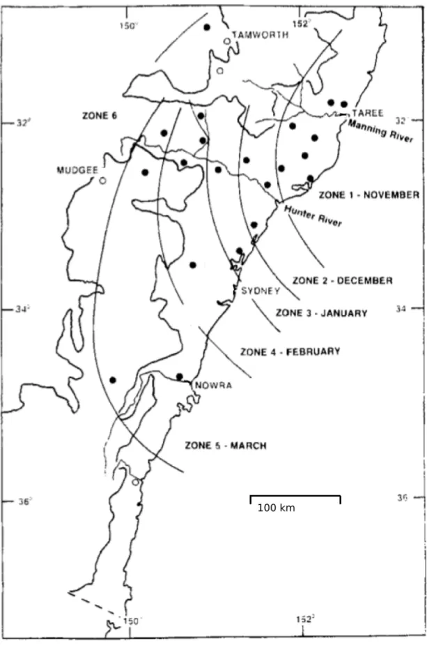
Population initialisation. The northern coastal area of the region being considered in this study is pictured in the north-east corner of the map shown in Figure 5 and contains an endemic population ofC. brevitarsis[11]. A viable population is known to persist throughout the mild winter period and subsequently increases as the weather warms during spring and summer [18]. This area is the source of midges which then spread southwards as the season progresses, as reported in the following [11,16–19]. The area containing endemic midge populations was initialised by the simulation model using the population dynamics sub-model as follows.
All cells in the region were seeded with adult and immature stages equally and the population dynamics process was run without any midge dispersal between cells. This simulation used 1-year temperature series for each cell (provided by the Australian Bureau of Meteorology), starting on 1st January 1991, which is summer in the Southern Hemisphere; 1991 was selected as this was the year preceding the year when mostC. brevitarsistrapping occurred [11]. Consecutive years were used so that the temper-ature data series ran continuously from the year used for population initialization (1991) through the year used as the primary comparison between simulated and observed midge spread (1992/3). This initialization procedure allowed for temperature differences between northern and southern areas of the modelled region to impact on population growth and, importantly, subsequent extinction. The low temperature activity parameter (LTAP) in the population dynamics sub-model was adjusted between successive applications of the initialization procedure until immature stage midges became locally extinct (in winter) in the same areas as reported in the literature [11,16,18,19] as being too cold to support overwintering. Specifically, the LTAP was adjusted in 1uC increments until a dividing line between the northerly overwintering population and southerly population (which became extinct) occurred south of the Hastings valley (31uS) but north of the Manning valley (31.9uS), see Figure 5. It should be noted that the LTAP value derived by the calibration process also depended on the value selected for the parameters ei and ea (described previously in Section 2.2).
However, while the overwintering behavior depended strongly on the LTAP with small (1uC) changes causing large differences in the overwintering area, it depended only weakly on ei and ea:
overwintering areas were similar foreiandeavalues spanning two
orders of magnitude.
The adult and immature population densities for each cell were recorded at the 1st October 1991 simulation cycle, and this population density map formed the initial conditions for the main simulations described in the results section. Video S1 shows an animated map of the population density during the calibration simulation. In performing this calibration procedure, it was noticed that the geographical occurrence of overwintering and occurrence is very finely balanced. Small changes in LTAP (or in the actual temperature times series) led to overwintering in the lower Hunter valley (see Figure 5), which is consistent with the fact that overwintering is intermittently observed in some years but not others [17].
Wind transport sub-model calibration. A series of simu-lations were conducted to determine the maximum wind transport
speed parameter, which accounts for midges possibly being transported by winds at high altitudes and higher speeds than the AWS recorded wind speeds (see Section 2.3 ‘‘Wind-borne dispersal’’). The population was initialized for 1stOctober 1991 as described above, and multiple simulations were run varying the wind speed transport multiplier over the range [0.0,5.0] in increments of 1.0. A value of 4.0 maximized the agreement between simulated and observed spread (as described below), and this value was used in subsequent spread experiments (further information can be found in Text S1, Table S1.5).
Simulation experiments. Experiments were conducted us-ing the model in the coastal area of NSW bounded by: 31.5 degrees south to 35 degrees south and 149 degrees east to 153.75 degrees east. The area was divided into a grid with 0.05 degree spacing (approximately 5 km), giving 12,350 individual cells. Cells with centroids in the ocean, urban areas of Sydney, Wollongong and Newcastle and national parks were marked as unsuitable habitats due to the need for cattle dung for ovipostioning (egg-laying). All other cells were deemed uniformly suitable C. brevitarsishabitats, assuming adequate cattle numbers to sustain the breeding cycle. More detailed cattle density heterogeneity data will be sourced when these modelling techniques are applied to BTV transmission in this region. Unless otherwise stated, simulations were run for 12 months from the beginning of October 1991, when midge populations begin to become active following winter.
Quantifying agreement between simulated and observed midge spread. We used aC. brevitarsistrapping data set that recorded the month during whichC. brevitarsiswas first detected at various sites in NSW in the summers of 1990/91, 1991/92 and 1992/93 [11]. In the publication describing the data set monthly time periods were reported, using data aggregated from weekly trapping time series data, which exhibited considerable noise at the weekly level. The output of each simulation run included the adult population density for each cell on each simulation day. For each of the trapping sites in the data set we determined the cell that contained the site, and determined the date on which the population rose above a trapping detection threshold parameter, which represented the minimum population density at which C.
Figure 5.C. brevitarsisspread arrival times as determined by trapping experiments.Lines denote arrival times ofC. brevitarsisderived from trapping data in New South Wales in 1991/2, classified by monthly zones. This figure is based on Figure 2 from [11]. Circles denote trapping site locations; filled circles indicate sites at whichC. brevitarsiswere detected, open circles where not detection occurred.
site at which simulated and observed arrival different by 2 months (e.g. December and February) was penalised four times more than a site with a 1-month disagreement (e.g. December and January). The significance value p is the probability of observing the level of agreement (kappa value) assuming that the true agreement is zero.
Results
3.1 Overview
Results presented in Section 3.2 illustrate the population dynamics generated by the model using seasonally varying temperatures. These highlight the effect which temperature has on C. brevitarsis population expansion and decline, as the temperature increases and then falls from spring through summer and into winter.
In Section 3.3, the effect of the two sub-models, viz. midge population dynamics and midge dispersal, is shown to capture seasonal midge incursions moving southwards along the NSW coast. If diffusive midge dispersal occurs without the addition of wind-driven dispersal, the simulated incursions fail to reproduce the rate of southerly spread observed by the field trapping programme [11,16,18,19]. With wind-dispersal added, monthly patterns for midge arrival times at the different trapping locations in NSW are (approximately) reproduced by the model. These simulated data confirm that both sub-models operating together replicate observed C. brevitarsis characteristics, that is, the dispersal of midges into ‘‘virgin territory’’, the subsequent temperature-dependent population establishment and growth in these areas, followed by decline and then extinction.
3.2 Population Dynamics
Using actual daily temperature data, the population dynamics sub-model was shown to be consistent with the C. brevitarsis
population dynamics data in the given locations and reported in [11,16,18,19], as follows.
Endemic populations where adults are present year-round can occur near the northern NSW state border, for example Byron Bay (latitude 28.64 south). Figure 6A shows the daily mean temperature and simulated population curves for the Byron Bay location over one year starting in January 1990. The data shown in Figures 6A, 6B and 6C were obtained by locating the simulation cell containing the site, and extracting the temperature and adult population density daily time series for that specific cell from the simulation used to establish the initial population (see Section 2.4 ‘‘Population initialisation’’). The simulated population curve shows that temperature and breeding activity are at a maximum in January and February, explicitly reflecting known temperature dependent population dynamics. The midge popu-lation grows during this period and peaks at the end of February. The population then slowly declines with declining temperatures, as the rate of newly emerging midges does not keep pace with the midge mortality rate. Temperature and breeding activity reaches a minimum in August. By the end of October the population begins to increase as the larvae from the increased breeding activity begin to emerge. The relationship between temperature (red) and the adult population (blue) can be seen clearly in Figure 6A.
Further south are areas in which the adult population disappears (i.e. falls below levels where it is detectable by a trapping program) during winter but where larvae survive and quickly re-establish adult populations once the temperature increases. Figure 6B shows temperature and population curves for Kempsey (latitude 31.08 south) which is approximately 350 km south of Byron Bay. In this location the simulated population curve during summer and autumn is similar to that described in
Figure 6A except that the population fluctuation is larger due to the greater seasonal temperature variation. At the coldest part of winter the adult population falls to zero: all adults die due to the low temperature and additionally no larvae emerge. Once the temperature increases however, surviving larvae emerge and establish a breeding cycle once more.
Further southwards ‘‘down’’ the NSW coast are areas in which imported populations can survive during summer and autumn but where longer winter cold periods render both the adult and immature populations extinct. Figure 6C shows temperature and population curves at Nowra (latitude 34.94 south, on the southern coast in Figure 5) which is approximately 570 km south of Kempsey. In this simulation a population is assumed to be present at the beginning of the year, due to movement from further north. The population grows in summer, declines in autumn, and the adult population becomes zero during winter. Somewhat later, the immature population (not shown) also becomes zero.
We note that midge populations reported in the literature from trapping programmes [18,20] are considerably more ‘noisy’ than the simulated population curves appearing above. We believe that this is primarily due to the relative spatial resolution of the simulation model compared to the area sampled by the traps. While the simulation model represents average midge density over a 5 km cell, each trap samples an area approximately 100 m wide, and so highly localised effects come into play, such as daily and weekly movement of cattle into and out of the area near the trap site.
3.3CulicoidesSpread and Population Dynamics
Midge trapping studies have documented the seasonal spread of
C. brevitarsis in NSW e.g. [11,16,18,19]. Typically, midge populations are detected in the Manning Valley coastal area in November (see Zone 1, Figure 5), having spread from the endemic areas further to the north. In the following months C.brevitarsis
midges are successively detected at increasing distances south-wards from the Manning Valley. Although prevailing winds are not predominantly from the north in this area, simulations show that periods of north or north-easterly winds are frequent enough to generate ‘‘spread events’’ that distribute C. brevitarsis into previously unoccupied territory, from which populations build and spread further. Winds in other directions also transport midges to the north and east; however these transport events do not impact the overall spread ofC. brevitarsis, as midges are spread back into areas they already occupy, or out to sea where there is no supporting habitat. The distance of southern spread varies from year to year due to weather variability, which includes the number and timing of significant southerly wind spread events, but the overall pattern remains similar; Figure 5 (based on Figure 2 from [11]) shows this spread during 1991/92.
along with a quantitative measure of agreement (Cohen’s kappa – see Section 2.4 ‘‘Quantifying agreement between simulated and observed midge spread’’). Table 1 also includes observed versus simulated midge arrival time comparisons for the seasons immediately prior to 1991/92, namely 1990/91 and 1992/93. Data from these additional years was not used in the calibration of the model, and thus serves as a proof-of-concept validation of the model.
A short animation of the simulated population dynamics and midge spread is provided in Video S2. The animation shows several clear wind transport events where midges are dispersed from locations with established populations to new areas, which then experience their own population growth and onward dispersal into previously midge-free areas. The animation also shows the seasonal cycle of the incursive midge population, with a
growth phase in summer and autumn, followed by disappearance of midges during the winter months, first from higher altitude inland areas which experience lower temperatures first, and then from the coastal area, starting from the south and proceeding northwards. New populations grow again in spring from overwintering populations in northerly, but not southerly areas.
3.4 Sensitivity analyses
In addition to the main experiments comparing observed midge spread to that generated by the simulation model, we also performed additional experiments to support the claim that a model combining temperature-dependent population dynamics and wind-borne dispersal is necessary to represent the seasonal incursiveC. brevitarsispopulation in NSW. Quantitative results of
Figure 6. Temperature and simulatedC. brevitarsispopulations.Daily mean temperatures are shown in red with scale on right axis. Adult midge population density shown in blue with scale on left axis. Population density is given in units where the maximum sustainable immature population density has a value of 100. Three time series were extracted from the population initialisation simulation (see Section 2.4 subsection ‘‘Population initialisation’’) for locations A: Byron Bay (latitude 28.64S), B: Kempsey (latitude 31.08S), and C: Nowra (latitude 34.94S).
doi:10.1371/journal.pone.0104646.g006
Figure 7. Simulated arrival times following midge dispersal and population establishment.A: Midge arrival times shown by colour for the months following 1stOctober. White (ocean) and grey indicates areas in which no midge population became established. B: Contours showing monthly arrival time Zones: Zone 1 November, Zone 2 December, Zone 3 January and Zone 4 February.
these experiments can be found in Text S1, Tables S1.8, S1.9 and S1.10.
In the C.brevitarsisliterature it is reported that the low winter temperatures in southern NSW prevent overwintering, and that when midges are detected in those locations this is a result of midges being transported from the north. As an initial test of our model, we considered an alternative hypothesis that midges overwinter in all locations where they are detected, and the apparent progression of midges from north to south is actually due to midges being detected at progressively later times due to slower population growth in southerly regions, reflecting temperature rises occurring later in the spring in the southern regions. This hypothesis was examined by running simulations without the midge transport sub-model, using a range of values for the LTAP value, which determines the locations in which overwintering will occur. We then compared the first simulated detection times of
midge populations which grow after overwintering, with the first detection times from the trapping data. We found that these simulation scenarios (with overwintering in all locations but without midge transport) could not reproduce the observed midge detection patterns. See Text S1, Table S1.8.
We next conducted simulations to determine if midge spread could be modelled as a purely diffusive local spread phenomena, without a wind-driven component. We found that in order to approximate the observed midge spread, the diffusion coefficient (representing the short-range, self-propelled flight behavior of midges) would have to be larger than any reported value for
Culicoides midges, such as presented in [45,47]. See Text S1, Table S1.9.
Finally, we examined how the temperature-dependent nature of the population dynamics affected the timing of midge spread. We found that a model using constant temperature could replicate the Table 1.Simulated and Observed Arrival Times.
1990/91 1991/92 1992/93
Number of sites (n) 25 24 13
agreement (kappa) 0.468 0.527 0.571
Significance (p)* 0.00205 0.00485 0.00661
Site observed/simulated arrival month
Buladelah 1/3 1/1 2/4
Bunyah 1/3 1/1 2/3
Bylong 5/6 5/3
-Camden 4/6 4/4
-Dartbrook 4/4 4/1
-Glenwilliam 2/4 1/1 3/3
Glouster 1/3 1/1 3/3
Goulburn 5/6 5/6
-Martindale 3/4 4/2
-Merriwa 5/3 5/2
-Morisset 2/6 2/3 3/4
Mudgee 6/6 -
-Murrurundi 4/4 4/2
-Nowra 4/6 5/6
-Ourimbah 3/6 3/3 4/4
Richmond 4/6 4/6 5/6
Scone 4/4 2/1
-Singleton 2/4 2/1 3/3
Tamworth-F - 6/1
-Tamworth-T - -
-Taree 1/2 1/1 1/3
Tea Gardens 1/4 1/1 2/4
Tocal 2/4 2/1 3/3
Upper Landsdown 1/2 1/1 1/2
Wallahbadah 4/3 -
-Warkworth 4/4 3/1
-Wauchope 1/1 1/1 1/2
Numbers given for observed and simulated C. brevitarsis arrival times denote the month after October i.e. Zone 1 November, Zone 2 December, Zone 3 January, Zone 4 February, Zone 6 March. A dash (-) indicates thatC. brevitarsiswere not observed (in reality or in simulations) in that year at that location; these sites were excluded from the analysis for that year.
* Significance p-value is the probability that the agreement kappa value would be found given that simulation and observation were uncorrelated i.e. if simulation results were random.
observed midge spread, however this model was inferior in several ways. Firstly, it is artificially sensitive to the starting date of the simulation, since population growth and spread occur from the beginning of the simulation; by contrast, the temperature dependent model is insensitive to the simulation start date, since spread begins only when temperatures allow population build-up in newly colonised areas. Secondly, while initial arrival times can be approximated with a constant temperature model, the final state of the midge population at the end of the simulation is very inaccurate, as with constant temperature there is no winter die-off of midges and midge activity occurs all through the year. This precludes the use of a constant temperature for multi-year simulations. See Text S1, Table S1.10.
Discussion
Models of insect vector population dynamics and movement are necessary when developing biologically plausible models of insect disseminated disease spread. The C. brevitarsis model presented here will be used in the future development of a BTV spread model and used to determine the effectiveness of interventions (e.g. vaccination, culling and/or movement bans) in achieving disease free status following an incursion into a previously disease free area [24]. Furthermore, the effects of longer term temperature changes, such as those caused by global warming are captured through the temperature dependencies included in the model. Changes in temperature ranges will potentially change the population dynamics and over-wintering ofC. brevitarsisin this region. The research challenge is to develop a modelling framework which supports the construction of realistic models which capture the fundamental features of the underlying physical system and, if possible, validate it using field-collected data, as is done in this study for the years 1990/91 and 1992/3 in Table 1.
The model described in this study was sufficiently realistic to permit us to address qualitative questions as to the nature of midge population growth and spread: that establishment of midge populations in southern areas in summer is inconsistent with an overwintering thesis but consistent with midges being transported from endemic areas in the north; and that this involves wind-blown midge transport and not solely self-propelled midge movement. The data in Table 1 indicate that simulated arrival times follow the same pattern appearing in the trapping data, with spread southward and westward from the endemic area as the months progress. However, midge arrival time predictions based on inferred initial populations and observed weather are not especially accurate, having Cohen’s kappa 0.527 (p = 0.00485). The major discrepancy between the simulated and observed spread is that in the simulation spread occurs rapidly to the west, over the Great Dividing Range to the NSW Tablelands, from where it spreads south, arriving all along the length of the Hunter Valley at the same time. The trapping data indicates that actual spread does not rapidly cross the Great Dividing Range, but occurs first southerly to the lower Hunter Valley area, and the progressively west up the valley. Limitations of the current model include the omission of rainfall, humidity and variable cattle density, all of which are lower in NSW inland areas, all which may contribute to this inaccuracy. These data-related issues could be addressed in future model developments.
The modelling mechanisms described above have been shown to model the key phenomena which underlie the spread of pathogen-carrying insect vectors and thus spread of the pathogens themselves. With appropriate adaptations these methods have application beyond the Culicoides vector and Bluetongue virus, with possible application to human viruses spread by mosquitoes,
such as dengue, chikungunya, and Japanese encephalitis [52,53]. They also have direct application to incursions of mosquito species into new territory, such as the recent spread of the Asian tiger mosquito Aedes albopictus, a competent vector for dengue and chikungunya, in southern Europe [54] and Australasia [55].
4.1 Related Research
Models of Bluetongue virus generally exclude inherently spatial landscape and habitat features which impact on Culicoides
population dynamics and movement, such as presented here. For example, the BTV transmission models presented in [26,27,56] rely on inter-farm BTV transmission being modelled by a distance kernel which implicitly includes vector dispersal and animal movement. The transmission model for between-farm spread required data from the 2006 northern European outbreak to estimate parameters; no location-explicitCulicoidesvector data was used and BTV outbreaks in different environments, such as different farm structures, insect vector habitats and climate regimes may not be directly modelled using this approach. BTV spread models with implicit vector populations do not allow for explicit modelling of the spatial spread of BTV via wind-moderated midge dispersal, nor BTV spread in areas where the presence of aCulicoidespopulation varies seasonally or from year to year.
Models which explicitly represent the effect of wind speed and direction on BTV spread via midge dispersal have been developed, in the study reported in [28] for example, where the spread of BTV cases is taken to be a surrogate for insect movement. In that model a more sophisticated wind model which included the effects of topography was utilized, compared to that adopted in this study. BTV outbreak data from southern France was used for model parameterization and no model of insect population dynamics was required, as BTV spread into areas with already-present competentCulicoidesspecies, in contrast to the vector incursion scenario presented here.