Comparison of simulated and reconstructed variations in East African hydroclimate over the last millennium

(1)

www.clim-past.net/12/1499/2016/ doi:10.5194/cp-12-1499-2016

Comparison of simulated and reconstructed variations in East

African hydroclimate over the last millennium

François Klein1, Hugues Goosse1, Nicholas E. Graham2, and Dirk Verschuren3

1_{Georges Lemaître Centre for Earth and Climate Research (TECLIM), Earth and Life Institute,}

Université catholique de Louvain (UCL), Belgium 2_{Hydrologic Research Center, San Diego, CA, USA}

3_{Limnology Unit, Department of Biology, Ghent University, Belgium}

Correspondence to:François Klein (francois.klein@uclouvain.be)

Received: 23 December 2015 – Published in Clim. Past Discuss.: 15 February 2016 Accepted: 20 June 2016 – Published: 13 July 2016

Abstract. The multi-decadal to centennial hydroclimate

changes in East Africa over the last millennium are stud-ied by comparing the results of forced transient simula-tions by six general circulation models (GCMs) with pub-lished hydroclimate reconstructions from four lakes: Challa and Naivasha in equatorial East Africa, and Masoko and Malawi in southeastern inter-tropical Africa. All GCMs sim-ulate fairly well the unimodal seasonal cycle of precipitation in the Masoko–Malawi region, while the bimodal seasonal cycle characterizing the Challa–Naivasha region is gener-ally less well captured by most models. Model results and lake-based hydroclimate reconstructions display very differ-ent temporal patterns over the last millennium. Additionally, there is no common signal among the model time series, at least until 1850. This suggests that simulated hydroclimate fluctuations are mostly driven by internal variability rather than by common external forcing. After 1850, half of the models simulate a relatively clear response to forcing, but this response is different between the models. Overall, the link between precipitation and tropical sea surface tempera-tures (SSTs) over the pre-industrial portion of the last millen-nium is stronger and more robust for the Challa–Naivasha re-gion than for the Masoko–Malawi rere-gion. At the inter-annual timescale, last-millennium Challa–Naivasha precipitation is positively (negatively) correlated with western (eastern) In-dian Ocean SST, while the influence of the Pacific Ocean appears weak and unclear. Although most often not signifi-cant, the same pattern of correlations between East African rainfall and the Indian Ocean SST is still visible when using the last-millennium time series smoothed to highlight

cen-tennial variability, but only in fixed-forcing simulations. This means that, at the centennial timescale, the effect of (natural) climate forcing can mask the imprint of internal climate vari-ability in large-scale teleconnections.

1 Introduction

(2)

1988; Hastenrath et al., 1993; Nicholson and Selato, 2000; Schreck and Semazzi, 2004; Hoell et al., 2014) or the Indian Ocean Dipole (IOD, e.g. Goddard and Graham, 1999; Saji et al., 1999; Webster et al., 1999; Clark et al., 2003; Ummen-hofer et al., 2009; Izumo et al., 2014). However, the mech-anisms involved are less clear. Goddard and Graham (1999) and Ummenhofer et al. (2009) suggested that an ocean driven change to the atmospheric Walker circulation impacts East African rainfall, while Klein et al. (1999) mentioned an at-mosphere driven change affecting both SSTs and rainfall. In any case, the 2011 drought was triggered by a strong La Niña event (IRI, 2010; Hoell et al., 2014) associated with a nega-tive IOD (Indian Ocean Dipole) (JAMSTEC, 2015) that re-sulted in drier than normal conditions in East Africa during the short rains at the end of 2010. The drought then worsened due to subsequent failure of the long rains in 2011 (Lyon and DeWitt, 2012).

Unlike short rains, the teleconnection between inter-annual East African long rains and the Indian and Pacific oceans is generally considered to be weak (e.g. Mutai and Ward, 2000; Pohl and Camberlin, 2006; Nicholson, 2014). However, failure of the long rains in 2011 was part of a progressive decline in long rains that has started around 1999 (Lyon and DeWitt, 2012) or even earlier (Funk et al., 2008), was associated with abrupt warming of the Indian Ocean (Funk et al., 2008; Williams and Funk, 2011) or of the western tropical Pacific (Merrifield, 2011; Lyon and De-Witt, 2012), also altering the Walker circulation. Merrifield (2011) and Lyon and DeWitt (2012) do not propose a specific cause for this warming. By contrast, Funk et al. (2008) and Williams and Funk (2011) attribute the large-scale shift in In-dian Ocean SSTs to anthropogenic forcing, and suggest that a warmer future climate will bring an increased frequency of drought conditions in tropical eastern Africa owing to further reductions in the long rains.

This hypothesis is at odds with general circulation mod-els (GCMs) showing that a warmer climate is associated with an increase in precipitation minus evaporation (P_-E₎ in the intertropical convergence zone (ITCZ), including the East African long rains (Seager et al., 2010; Laîné et al., 2014). Other model-based studies (McHugh, 2005; Shongwe et al., 2011; Kirtman et al., 2013) furthermore suggest that increasingly wetter rainy seasons in East Africa are due to a weakening of the Walker circulation, likely linked to an-thropogenic warming (Vecchi et al., 2006; Vecchi and So-den, 2007). This is corroborated by some observations which appear to show a weakening of the Walker circulation al-ready since the mid-19th century (Vecchi et al., 2006). How-ever, there is no agreement on that in observation-based stud-ies, as illustrated by L’Heureux et al. (2013) who found a multi-decadal strengthening of the Walker circulation over the same period. In addition, some regional climate mod-els forced at the boundaries by ensemble-mean GCM results are not consistent with GCMs in that they show a reduction

rather than increase in the long rains (Vizy and Cook, 2012; Cook and Vizy, 2013).

The inability of the GCMs in simulating the observed re-cent downward trend of the long rains implies either that it is part of (multi-)decadal natural variability (Lyon and DeWitt, 2012; Yang et al., 2014; Lyon, 2014), or that the GCMs in-adequately represent the climate processes occurring in the region and the response to anthropogenic forcing. In this context, it is crucial to assess the performance of GCMs in simulating East African rainfall. Existing studies on this sub-ject (e.g. Conway et al., 2007; Anyah and Qiu, 2012; Otieno and Anyah, 2012; Yang et al., 2014) have reached contrast-ing conclusions dependcontrast-ing on the region or spatial scale, or on the variables and models considered. Specifically, they showed that the mean seasonal cycle of precipitation is rea-sonably well simulated by the majority of GCMs, but that there is a large spread among them in capturing the actual dominant peaks where rainfall is bimodal (Anyah and Qiu, 2012; Otieno and Anyah, 2012). Additionally, most models appear to have significant biases in monthly mean precip-itation, and the observed link between East African rainfall and Indian Ocean SST is often not well represented (Conway et al., 2007; Yang et al., 2014).

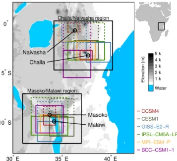
All the above studies are limited to the recent past where direct measurements of precipitation exist. However, the pe-riod considered, which ranges from the last few decades to 150 years at most, is not sufficient to capture the multi-decadal variability that is thought to be an important compo-nent of East African hydroclimate (Verschuren, 2004; Tier-ney et al., 2013). Therefore, to complement those studies, our goal is to extend this analysis to the last millennium by analysing proxy records of past hydroclimatic change over this period in conjunction with simulations performed in the framework of the third phase of the Paleoclimate Mod-elling Intercomparison Project (PMIP3; Otto-Bliesner et al., 2009) and of the fifth phase of Coupled Model Intercompari-son Project (CMIP5; Taylor et al., 2012). All hydroclimate proxy records available from eastern Africa that are both well-dated and span the last millennium with sufficient time resolution are based on lake-sediment records (Verschuren, 2004). In this study, we consider proxy records describing the water-balance history of four East African lakes: Lake Challa and Lake Naivasha in eastern equatorial Africa, and Lake Masoko and Lake Malawi in southeastern (but still inter-tropical) Africa (Fig. 1). These four lake records are part of the East African hydroclimate synthesis recently achieved by Tierney et al. (2013), and all characterized by strong multi-decadal to centennial variability. As a consequence, the present study focuses on relatively long-term hydroclimate changes, and on variation in annual means rather than indi-vidual rainy seasons, in contrast with model and observation-based studies about variation in recent East African rainfall (e.g. Anyah and Qiu, 2012; Yang et al., 2014).

(3)

last millennium to define whether the simulated changes re-flect the forcing of external climate drivers and to assess the stability of large-scale teleconnections between East African rainfall and global SSTs. This paper is structured as follows. In Sect. 2 we introduce the model experiments and proxy-based reconstructions. In Sect. 3 we evaluate the comparative performance of six different GCMs to simulate the seasonal cycle of rainfall over the study regions and its teleconnection to tropical SSTs over the recent period. In Sect. 4 we anal-yse the results of model simulations spanning the last mil-lennium. The contribution of forced and internal variability on those simulated hydroclimate changes and the stability of large-scale teleconnections are finally investigated in Sect. 5, followed by a discussion and conclusions in Sect. 6.

2 Data and methods

2.1 PMIP3/CMIP5 model experiments

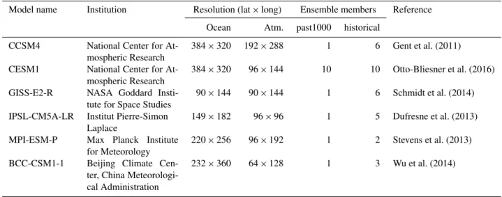
Climate model simulations from PMIP3 (Otto-Bliesner et al., 2009) and CMIP5 experiments (Taylor et al., 2012) were ob-tained from the Program for Climate Model Diagnosis and Inter-comparison (PCMDI; http://pcmdi9.llnl.gov) and the Earth System Grid (www.earthsystemgrid.org) archives. The six GCMs selected (Table 1) are those for which the diagnos-tic variables of interest, i.e. precipitation, actual evaporation and SST, were available at the time of our analysis, for both past1000 (850–1850 AD) and historical (1850–2005) peri-ods, as well as for pre-industrial control runs.

Although not continuous, except for CESM1 and MPI-ESM-P, the first ensemble members (r1i1p1) of past1000 runs were merged with the corresponding historical simu-lations to obtain results spanning the period 850–2005 AD. The impact of the discontinuity is probably limited since it falls within the range of internal climate variability for sur-face variables in all cases. The simulations are driven through the last millennium by both natural (orbital, solar, volcanic) and anthropogenic (well-mixed greenhouse gases, ozone, tropospheric aerosols, land use) climate forcings. Earth’s or-bital parameters vary according to the calculations of Berger (1978). Depending on the model, different reconstructions of solar irradiance variability are applied. All models except CESM1 and GISS-E2-R use the reconstruction by Vieira and Solanki (2009) from 850 to 1609 and by Wang et al. (2005) from 1610 to 2005. CESM1 uses the reconstruction by Vieira et al. (2011) with the spectral variations and “11-year” solar cycle from Schmidt et al. (2012), whereas GISS-E2-R uses the Steinhilber et al. (2009) reconstruction until 1849 and the Wang et al. (2005) one from 1850 onwards.

The forcing related to volcanic aerosols is derived from Crowley and Unterman (2013) in GISS-E2-R and MPI-ESM-P and from Gao et al. (2008) in the four other GCMs. Re-constructed and observed changes in the major greenhouse gases driving past1000 (Flückiger et al., 2002; MacFarling Meure et al., 2006) and historical (Hansen and Sato, 2004)

simulations, ie. CO2, CH4and N2O, are the same in all mod-els. Anthropogenic changes in land use/land cover over the last millennium are based on the reconstruction of Pongratz et al. (2008) in MPI-ESM-P, of Pongratz et al. (2008) fol-lowed by the reconstruction of Klein Goldewijk and van Drecht (2006) for the historical period in GISS-E2-R and of Pongratz et al. (2009) followed by the reconstruction of Hurtt et al. (2011) for historical time in CCSM4 and CESM1. BCC-CSM1-1 and IPSL-CM5A-LR do not con-sider any change in land use/land cover, whose distribution is fixed to the pre-industrial value. Tropospheric ozone and aerosols variations are also taken into account in historical experiments in CCSM4, CESM1, GISS-E2-R, MPI-ESM-P and BCC-CSM1-1, and are all based on the data set described in Lamarque et al. (2010). These changes are however ne-glected in IPSL-CM5A-LR, which considers a constant con-centration fixed at the pre-industrial level. More information on the climate-forcing reconstructions used to drive past1000 experiments and on their implementation can be found in Schmidt et al. (2011) and Schmidt et al. (2012).

2.2 Proxy-based hydroclimate reconstructions

(4)

Table 1.Modelling centres, parameters and references of the PMIP3/CMIP5 models used in this study.

Model name Institution Resolution (lat×long) Ensemble members Reference Ocean Atm. past1000 historical

CCSM4 National Center for At-mospheric Research

384_×320 192_×288 1 6 Gent et al. (2011)

CESM1 National Center for At-mospheric Research

384×320 96×144 10 10 Otto-Bliesner et al. (2016)

GISS-E2-R NASA Goddard Insti-tute for Space Studies

90×144 90×144 1 6 Schmidt et al. (2014)

IPSL-CM5A-LR Institut Pierre-Simon Laplace

149×182 96×96 1 5 Dufresne et al. (2013)

MPI-ESM-P Max Planck Institute for Meteorology

220×256 96×192 1 2 Stevens et al. (2013)

BCC-CSM1-1 Beijing Climate Cen-ter, China Meteorologi-cal Administration

232×360 64×128 1 3 Wu et al. (2014)

meet minimum criteria of continuity and hydroclimate signal strength. However, a critical review of all available records might nevertheless refine the spatial structure of documented hydroclimate changes, and allow further assessment of the robustness of broad-ranging climate-dynamic inferences.

The 1000-year time series representing hydroclimate vari-ation in the Lake Challa region developed by Tierney et al. (2013) is the first principal component of the composite vari-ation in three moisture-balance proxies, namely the branched and isoprenoidal tetraether index BIT (a presumed indica-tor of total annual rainfall: Verschuren et al., 2009; Buck-les et al., 2016); δD _{in the leaf waxes of terrestrial plants} (an isotopic proxy for rainfall source and intensity: Tierney et al., 2011); and varve thickness (a proxy for variation in dry-season length and windiness: Wolff et al., 2011). This first principal component accounts for 40 % of the variance in the data (supplementary material of Tierney et al., 2013). The time series from Lake Naivasha is a lake-level reconstruction based on sediment lithostratigraphy (Verschuren, 2001), sup-ported by salinity reconstructions based on fossil diatom and midge assemblages (Verschuren et al., 2000). The hydrocli-mate record from Lake Masoko is inferred from the low-field magnetic susceptibility of the sediment, which is a proxy for lake-level changes and/or wind stress. Two such records are available for this lake, one that goes back to −43 300 AD (Garcin et al., 2006) and one that starts around 1500 AD (Garcin et al., 2007). The Masoko time series in this paper is obtained from Tierney et al. (2013), who used the last mil-lennium of the longer record but with age-depth tie-points translated from the shorter record (Anchukaitis and Tierney, 2012). Finally, the hydroclimate record from Lake Malawi is deduced from the mass accumulation rate of the terrigenous sediment fraction, presumed to be a runoff proxy (Brown and Johnson, 2005; Johnson and McCave, 2008). Supple-ment Table S1 provides more information about each of these

four proxy records. Although these records are derived from different proxies, their time series can all be qualitatively viewed as smoothed versions of the local moisture-balance history of the corresponding sites.

3 Evaluation of model performance over the period

1979-2005

3.1 Mean seasonal cycle of precipitation

This section assesses the ability of various GCMs to repro-duce the observed mean state and seasonal cycle of East African rainfall. Although similar analyses have been per-formed previously (e.g. Conway et al., 2007; Anyah and Qiu, 2012; Otieno and Anyah, 2012; Yang et al., 2014), it is im-portant to repeat it here focusing specifically on the areas where our four study sites are located (Fig. 1).

(5)

Cli-Figure 1.Location of lakes Challa, Naivasha, Masoko and Malawi in East Africa, along with the individual grid cells containing each of these four sites in six different CMIP5 models (dashed (plain) boxes for the grid cells that contain the lakes Naivasha and Ma-soko (Challa and Malawi)), and the two larger regional domains over equatorial East Africa (Challa–Naivasha region) and south-eastern inter-tropical Africa (Masoko–Malawi region). Topography from Amante and Eakins (2009).

mate Prediction Center (CPC) Merged Analysis of Precipita-tion data set (CMAP; Xie and Arkin, 1997) covers the same period at identical spatial resolution but combines rain-gauge data and different satellite estimates with NCEP/NCAR re-analysis results in gaps. Finally, NOAA’s Precipitation Re-construction over Land data set (PREC/L Chen et al., 2002) is based only on rain-gauge data and covers the period from 1948 to the present with a spatial resolution of 0.5◦×0.5◦.

Due to the seasonal north-south migration of the ITCZ across the equator, East African rainfall is characterized by a strong annual cycle that differs from one location to an-other (Nicholson, 1996; Otieno and Anyah, 2013; Yang et al., 2015). The seasonality of rainfall is bimodal over equatorial sites such as Lake Challa and Lake Naivasha, with two rainy seasons occurring in March to May (long rains) and in Oc-tober to December (short rains), while it is unimodal in the southeastern lakes Masoko and Malawi, with a maximum be-tween November and April during the austral summer (bar charts in Fig. 2). The observed mean monthly rainfall in each of the four study areas over the period 1979–2005 serves as our reference frame to compare the success of individual GCMs in simulating the present-day seasonal cycle, using model results from the individual grid cells which include the lakes (Fig. 1).

For Lake Naivasha (Fig. 2a), simulated monthly mean pre-cipitation is characterized by a large spread among models. Observed short rains over this lake are relatively well

sim-ulated by most models, except by GISS-E2-R and IPSL-CM5A-LR which, respectively, strongly overestimate and underestimate them. During the other seasons, simulated pre-cipitation over Lake Naivasha is underestimated by all mod-els except GISS-E2-R, including during the main rainy sea-son in boreal spring. Regarding the average of monthly mean precipitation throughout the year at Lake Challa (Fig. 2b), three models are within the range of the observations: CCSM4, CESM1 and BCC-CSM1-1. Most models under-estimate the long rains except CESM1 and GISS-E2-R, al-though in these two models this rainy season is delayed by one month compared to observations. In contrast with the observations, all models show highest rainfall in October or November rather than April, but the spread is again large. These differences between models during the short rains are consistent with biases at larger spatial scales noted in previ-ous studies of the East African region. Anyah and Qiu (2012) and Yang et al. (2014) indeed showed that, despite a large spread among CMIP3 and CMIP5 models, most of them tend to underestimate and to shift by one month the long rains, and to overestimate the short rains. Agreement among models and between models and observations is much higher in Lake Masoko and Malawi (Fig. 2c–d). Both the rainy and dry sea-sons are well simulated, although the amount of rain is over-estimated by CCSM4 and IPSL-CM5A-LR during the rainy season. Overall, climate models used in this study are thus able to represent the unimodal rainfall seasonality character-izing the region encompassing lakes Masoko and Malawi, while the timing and the magnitude of the two rainy sea-sons characterizing the region encompassing lakes Challa and Naivasha are in general less well captured.

Comparing model results and data at individual grid cells can be questionable since model skill at this scale is often very limited. For instance, a small shift in the spatial struc-ture of the simulations compared to the observations can lead to a large difference in precipitation. Local topographic fea-tures not well represented at the grid scale may also have a significant impact. Besides, the surface areas of the grid cells which include the lake sites strongly differ from one model to another (Fig. 1). To get rid of the problems linked to differ-ences in spatial resolution and to remove local noise in favour of more regional patterns, it seems better to analyse, instead of individual grid cells, larger regions presenting common characteristics as discussed in the next section.

3.2 Link between individual grid cells and the larger spatial domains selected for analysis

(6)

R

a

in

fa

ll (

m

o

n

th

)

Jan Feb Mar Apr MayJun Jul Aug Sep Oct NovDec Mean Naivasha

(a)

0 50 100 150 200 250 300

Jan Feb Mar Apr May Jun Jul Aug Sep Oct NovDec Mean Challa

(b)

R

a

in

fa

ll (

m

o

n

th

)

Jan Feb Mar Apr MayJun Jul Aug Sep Oct NovDec Mean

Masoko

(c)

0 50 100 150 200 250 300 350

Jan Feb Mar Apr May Jun Jul Aug Sep Oct NovDec Mean

Malawi

(d)

CCSM4 (6)

GISS-E2-R (6)

MPI-ESM-P (2) IPSL-CM5A-LR (6) CESM1(10) Observations (4)

Multimodel mean bcc-csm1-1(3)

-1

Figure 2.Mean monthly rainfall over lakes Naivasha, Challa, Masoko and Malawi(a–d)in observations (bar plots) and in six CMIP5 models (curves) over the period 1979–2005. The number of data sets (for the observations) or ensemble members (for the models) used in each case is shown in brackets. Error bars and shaded areas represent the range of those observations or ensemble member values.

12.2◦S and 31 to 37◦E, referred to as the Masoko–Malawi region; Fig. 1). Note that shifting or changing the size of these two regions to some extent does not produce substantial changes in the results.

However, using larger grid boxes raises the issue of whether the proxy-based reconstructions that are compared to model results over the last millennium are representative of these larger spatial domains. Fig. 3 shows the correlation between modelled mean annual rainfall in the individual grid cells containing the four lake sites and the two larger do-mains defined for our analysis, for both the recent period and the last millennium. Changes in precipitation within the grid cell containing Lake Masoko, within the grid cell contain-ing Lake Malawi and within the larger box representcontain-ing the Masoko–Malawi region are highly and significantly corre-lated for all models and observations, and for both periods. Rainfall over Lake Challa, Lake Naivasha and the Challa– Naivasha region is also positively correlated in both periods for each source of information.

Observed recent rainfall over Lake Challa, Lake Naivasha, and the Challa–Naivasha region shows no or only a weakly positive relationship with rainfall over Lake Masoko, Lake Malawi and the Masoko–Malawi region, underscoring the climatic dichotomy characterizing East Africa. Note that no negative correlation is found except very weak ones in GISS-E2-R between rainfall over Lake Challa and rainfall over Lake Masoko, Lake Malawi and the Masoko–Malawi region. The dipole between the eastern coastal “Horn of Africa” re-gion and the interior rift-valley rere-gion highlighted in Tierney et al. (2013) is thus not observed at the annual timescale con-sidered here. Although the correlations are quite similar for the recent period and the last millennium, they are somewhat

BCC-CSM1-1

850_–18 50 AD 197_9–2

005_AD

(7)

higher in the former. This may be caused by the present-day anthropogenic forcing that induces a coherent response be-tween the selected locations within each model.

Overall, both observations and model results show that the two selected regions are on the one hand characterized by dif-ferent patterns of temporal variability and, on the other hand, representative of the individual grid cells containing the lake sites, not only regarding annual precipitation changes over the recent period and the last millennium, but also regard-ing seasonal cycles and annual mean absolute values (not shown).

3.3 Large-scale teleconnections

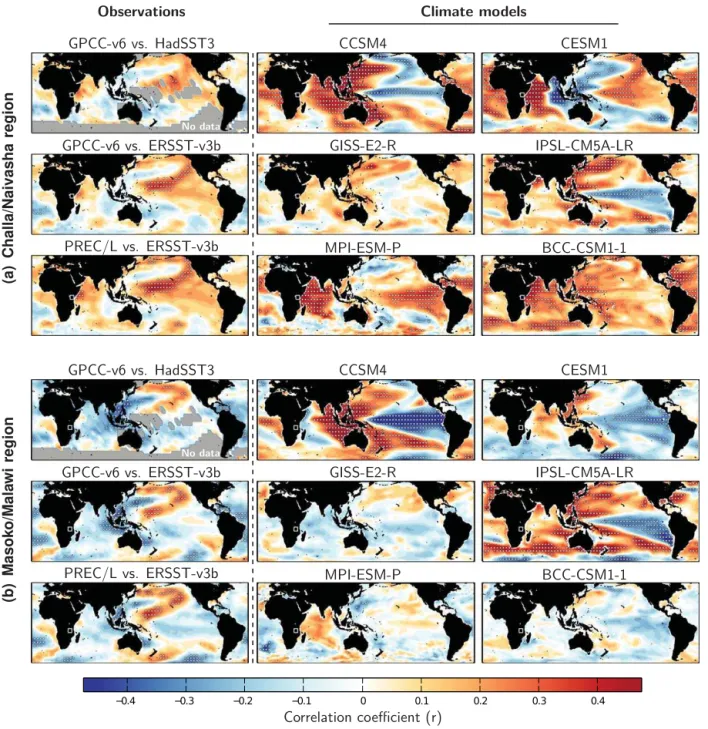
In addition to the evaluation of the mean state, it is impor-tant to assess the ability of climate models to represent the observed patterns associated with the inter-annual variability of East African rainfall. Although it is not our goal here to study the mechanisms responsible for the simulated variabil-ity, this is illustrated by analysing the correlations between East African precipitation and tropical SSTs. The latter is in-deed considered as a direct driver of precipitation over East Africa (e.g. Goddard and Graham, 1999; Ummenhofer et al., 2009). Two different SST data sets are used: version 3 of the Hadley Centre data set (HadSST3; Kennedy et al., 2011a, b), based on in situ measurements covering the period from 1850 to 2015 on a 5◦×5◦grid, and version 3b of the Extended Re-constructed Sea Surface Temperature data set (ERSST-v3b; Smith et al., 2008), also based only on in situ data, which covers the period 1854 to 2015 on a 2◦_×₂◦_{grid. Since the}

proxy-based reconstructions used in this study are considered to represent mean annual conditions, interest is here mainly on mean annual results. However, mean annual results for East Africa’s hydroclimate represent a combined picture, as the relative amplitudes and the strength and character of tele-connections between East African rainfall and tropical SSTs at the inter-annual timescale are different from one season to another.

For both regions, the largest correlations between observed rainfall and SSTs are found during the boreal autumn (OND), with the well-known pattern of positive (negative) correlation between East African rainfall and western (eastern) Indian Ocean SSTs, as well as SSTs in the central/eastern (western) equatorial Pacific (Supplement Figs. S1 and S2 OND), which resembles the SST pattern during an El Niño phase of ENSO and a positive phase of the IOD. This period corresponds to the short rains in Challa–Naivasha and to the start of the sin-gle rainy season in Masoko–Malawi farther south (Fig. 2). For the other seasons, the spatial pattern of correlations dif-fers between the two study areas, with the greatest difference occurring during boreal winter (JFM). In Challa–Naivasha, where rainfall is relatively low during this transition period between the short rains and the long rains, it appears to be positively correlated with SSTs over the central/north Indian Ocean (Fig. S1 JFM). In contrast, just a few isolated

signif-icant correlations are found between rainfall in boreal win-ter over Masoko–Malawi and tropical SSTs (Fig. S2 JFM), although this period marks the annual maximum in precipi-tation (Fig. 2). Teleconnections to tropical SSTs are weak in both regions during the boreal spring (AMJ; Figs. S1 and S2 AMJ), which corresponds to the long rains in Challa– Naivasha and to the end of the rainy season in Masoko– Malawi; and are also weak during the boreal summer (JAS; Fig. S1 and S2 JAS), which is the principal dry season in both regions (Fig. 2).

When considering mean annual results, the correlations between observed precipitation over the Challa–Naivasha re-gion and SSTs show a pattern similar to that during the short rains, although damped, with positive correlations in the western Indian Ocean and central/eastern tropical Pa-cific and negative ones centred on Indonesia (Fig. 4a left). In contrast, the correlations between Masoko–Malawi rainfall and SSTs after computing annual averages are mostly weak and non-significant in the Indian Ocean and negative over the Indonesian region while some zones in the Pacific show positive correlations (Fig. 4b left), even though the correla-tions pattern for boreal autumn (OND) rainfall is similar to that found using precipitation over Challa–Naivasha. In both cases, the spatial pattern of correlations derived from the dif-ferent combinations of data sets show very similar results, with spatial correlations of the obtained patterns always ex-ceeding 0.80.

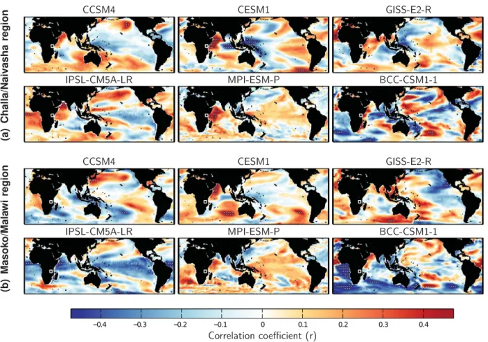
Out of the six GCMs, only CESM1 and MPI-ESM-P seem to simulate relatively well the spatial pattern of correlations between Challa–Naivasha rainfall and SSTs (Fig. 4a). How-ever, the match with observations is far from perfect as shown by the relatively low correlation coefficients between simu-lated and observed rainfall SST correlation maps, with values equal to 0.27 and 0.16, respectively (Table S2). GISS-E2-R, IPSL-CM5A-LR and BCC-CSM1-1 display totally different patterns compared to observations, and CCSM4 even simu-lates an opposite pattern, with positive (negative) correlations between simulated precipitation over the Challa–Naivasha area and the eastern Indian Ocean (central/eastern Pacific).

(8)

0.4 0.3 0.2 0.1 0 0.1 0.2 0.3 0.4 GPCC-v6 vs. HadSST3

No data GPCC-v6 vs. ERSST-v3b

PREC/L vs. ERSST-v3b

CCSM4 CESM1

GISS-E2-R IPSL-CM5A-LR

MPI-ESM-P BCC-CSM1-1

Observations Climate models

(a)

Challa/Naivasha

region

GPCC-v6 vs. HadSST3

No data GPCC-v6 vs. ERSST-v3b

PREC/L vs. ERSST-v3b

CCSM4 CESM1

GISS-E2-R IPSL-CM5A-LR

MPI-ESM-P BCC-CSM1-1

(b

)

M

a

s

o

k

o

/M

a

la

w

i

re

g

io

n

Correlation coefficient (r)

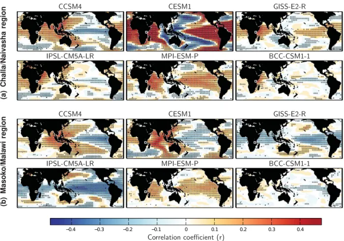
Figure 4.Pearson correlation coefficients between mean annual rainfall over the Challa–Naivasha region (a, upper three rows) or Masoko– Malawi region (b, lower three rows) and global SSTs in observations and climate models (here, only the first member r1i1p1 is used) for the period 1950–2000. In areas overprinted with white circles, a null hypothesis of no correlation can be rejected at the 5 % level. No data are available from grey areas.

real winter, no correlation is found when considering annual mean results.

Overall, most climate models fail to simulate observed teleconnections of Challa–Naivasha and of Masoko–Malawi rainfall to large-scale SST patterns at the inter-annual scale. Annual smoothing makes these teleconnections complex and of relatively limited magnitude, especially for Masoko– Malawi rainfall. However, this cannot by itself explain the low model performance since their skill is not greatly

(9)

MPI-Drier

Drier

Wetter

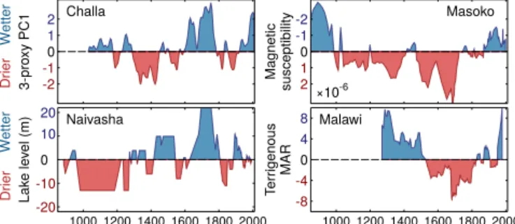
Figure 5. Lake-based moisture-balance reconstructions used in this study; references with details on the proxies are provided in Sect. 2.2. Ordinate axes for each proxy are oriented such that wetter (drier) hydroclimate conditions point upward (downward).

ESM-P and CESM1 thus tend to stand out by their posi-tive correlation with annual observations in both regions and only in Challa–Naivasha, respectively, for the right reasons. These mitigated results are, to some extent, consistent with the study of Rowell (2013). Indeed, although using differ-ent methodologies and selected areas, this author has shown that the teleconnections between rainfall over central East Africa (roughly corresponding to the Masoko–Malawi re-gion) and both equatorial Pacific and Indian Ocean SSTs are particularly hard for CMIP5 models to reproduce. Fur-thermore, Rowell (2013) reached a similar conclusion about the teleconnections between rainfall over the greater Horn of Africa region, which includes the Challa–Naivasha region, and equatorial Pacific SSTs.

4 Reconstructed and simulated hydroclimate over

the last millennium

4.1 Hydroclimate changes deduced from proxy-based reconstructions

Notwithstanding chronological uncertainty, the Challa and Naivasha proxy records display clear differences during the first four centuries of the last millennium. In particular, the former shows a general drying trend while the oppo-site is recorded in the latter (Fig. 5). However, from around 1400 AD the conditions inferred from these two records are similar: both show relatively dry conditions followed by a wetting trend peaking between about 1700 and 1750 AD. After this peak, both hydroclimate reconstructions depict an abrupt transition towards a dry period in the early 19th cen-tury, followed by smaller-scale hydroclimate fluctuations at Naivasha and a clear wetting trend at Challa.

Contrasting with Challa and Naivasha, lakes Masoko and Malawi both show a general drying trend culminating around 1700 AD, before an increase in humidity towards the present. However, (multi-) decadal hydroclimate changes overlying these long-term trends often strongly differ between the two records.

The differences between the Challa and Naivasha recon-structions on the one hand and between the Masoko and Malawi reconstructions on the other can be viewed as a measure of how representative these records are of hydro-climatic variability within each region. Certainly, the differ-ences partly reflect real local features due to different expo-sure to the principal seasonal moisture sources related to dis-tance to the sea, topography etc. However, a significant frac-tion of the difference observed within each pair of records is likely due to uncertainty in the reconstructions themselves, due to the compound effects of (i) dating uncertainty in these lake-based proxy records, (ii) differences in hydrology and local catchment processes influencing a lake’s (or in the case ofδD_{, its surrounding vegetation) sensitivity to climate,} and/or iii) the fact that the used hydroclimate proxies have a specific and different relationship with temporal variation in our target of reconstruction, i.e. the climatic moisture bal-ance. Importantly, the point here is that the differences be-tween the two pairs of records are larger than those within each pair. Each pair can thus be considered as representative of a distinct hydroclimatic region (cf. Tierney et al., 2013).

4.2 Interpretation of proxy-based reconstructions from a model perspective

Lakes are complex hydrological systems. To understand their dynamics, it is necessary to account for the inflow and out-flow from rivers and surface runoff, rainfall on the lake surface, evaporation from the lake surface, groundwater in-flow and/or outin-flow, as well as interactions with the aquifer surrounding the lake (e.g. Becht and Harper, 2002). These processes are not represented directly in relatively coarse-resolution GCMs. These models simulate the large-scale moisture balance, i.e. precipitation minus actual evaporation (P_-E_{), the latter depending on potential evaporation and soil} moisture content. Each of the sedimentary proxies used in the lake-based climate reconstructions can be qualitatively interpreted as smoothed versions of the local-to-regional cli-matic moisture balance, at least when considered on multi-decadal to centennial timescales. P_-E _{is thus the model} variable that has been chosen here for comparison with the reconstructed histories of lake-level fluctuation, catchment runoff or drought-season severity, depending on the lake (see Sect. 2.2). This section describes the relative contributions of rainfall and of evaporation inP_-E_{, which allows} know-ing whether the respective regions containknow-ing each record are more influenced by precipitation or evaporation.

(10)

mod-(a) (b)

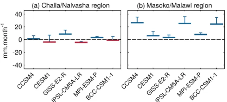
Figure 6.Mean annual precipitation minus mean annual evapora-tion (horizontal bars), and standard deviaevapora-tion of annual precipitaevapora-tion minus the standard deviation of annual evaporation (vertical bars) using the entire last-millennium results (850–2005) for each GCM. Red (blue) colour means that evaporation (precipitation) dominates.

Table 2.Pearson correlation coefficients between simulated rainfall and simulated evaporation in the Challa–Naivasha and Masoko– Malawi regions over the pre-industrial portion of the last millen-nium (850–1850 AD).

Challa–Naivasha Masoko–Malawi

CCSM4 0.66∗ 0.09∗

CESM1 0.57∗ 0.35∗

GISS-E2-R 0.71∗ 0.95∗

IPSL-CM5A-LR 0.91∗ 0.69∗

MPI-ESM-P 0.68∗ 0.62∗

BCC-CSM1-1 0.88∗ 0.70∗

∗Significant at the 5 % level.

els show positive P_-E _{values for the Masoko–Malawi} re-gion during the last millennium (Fig. 6b). The higher P -E _{for Masoko–Malawi compared to Challa–Naivasha is as} expected due to higher precipitation, which more than com-pensates for higher evaporation and thus leads to larger river runoff.

If we consider the standard deviation of variation inP _and E _{through the last millennium, there is a consensus among} models that P _{is more variable from year to year than} E_, for both regions (vertical bars in Fig. 6, which all plot up-wards). This implies that most changes of P_-E _{over time} are due to changes in precipitation. Differences between the standard deviation ofP _{and of}E_{are also generally greater in} Masoko–Malawi. This can be explained in all models except GISS-E2-R by a weaker relationship between P _andE _in this region than in Challa–Naivasha, as evidenced by weaker correlation coefficients (Table 2). Higher correlations indeed mean that a change in P _{is more often accompanied by a} similar change inE_{, which tends to bring variances closer.}

These results are robust throughout the last millennium where they remain relatively stable over time, even during the recent past where one could expect evaporation to in-crease relative to precipitation due to anthropogenic warm-ing (not shown). Moreover, rainfall still has a dominant role

in explaining changes inP_-E _{when considering timescales} longer than annual, since approximately the same picture is observed when filtering model results using a loess method with a window of 100 years (not shown).

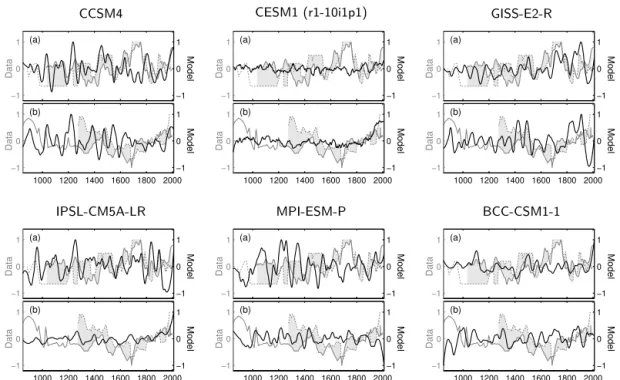
4.3 Comparison between reconstructions and model results

As briefly discussed in Sect. 4.2, the link between simulated and reconstructed variables is only indirect, which means that the magnitude of simulated P_-E _{that should best fit} the reconstructions is unknown. Consequently, the focus in this comparison is on common relative changes, rather than on their magnitude in absolute values. For better readability of the figures, each time series has been linearly standard-ised so that the maximum of the absolute values equals 1. A 100-year smoothing is applied to the model results in order to resemble temporal variability in the reconstructions. Our choice of a 100-year smoothing window is partly subjective, since the resolution of the proxy-based reconstructions varies through time due to a non-linear relationship between sedi-ment depth and age. However, using other window widths for this smoothing does not lead to major changes in the results. Despite this smoothing, most model curves do not show any distinct long-term trend in the past millennium as ob-served in the proxy-based reconstructions, and have weaker fluctuations at the centennial scale than the reconstructions (Fig. 7). The correlation coefficients between model results and reconstructions, computed annually using interpolations for the reconstructed time series, are presented in Table S3. Most coefficients are low and non-significant at the 0.05 % level, and can be for a same site either positive or negative depending on the models, which implies that there is no com-mon signal between models and data but neither acom-mong mod-els.

No individual site is characterized by an overall better agreement between model and data since the averages of cor-relation coefficients for each lake are close to zero. Further-more, taking the four sites into account, no model appears to match substantially better the reconstructions than another. Nevertheless, some isolated positive correlations should be mentioned: CESM1 shows one positively and statistically significant correlation of 0.43 with the average of the recon-structions from Masoko and Malawi, and GISS-E2-R cor-relates with the average Challa–Naivasha time series with a coefficient of 0.38.

(11)

af-−1 0 1 (a) Model Data −1 0 1 −1 0 1 (b) Model Data

1000 1200 1400 1600 1800 2000 −1 0 1 −1 0 1 (a) Model Data −1 0 1 −1 0 1 (b) Model Data

1000 1200 1400 1600 1800 2000 −1 0 1

CCSM4 CESM1 (r1-10i1p1) GISS-E2-R

IPSL-CM5A-LR MPI-ESM-P BCC-CSM1-1

Figure 7.Comparison between last-millennium time series of the reconstructions (in grey) and ofP-Esimulated by six GCMs (in black) averaged over the Challa–Naivasha region(a), with the Naivasha record shown as dashed line and the Challa record as solid line; and over the Masoko–Malawi region(b), with the Malawi record shown as dashed line and the Masoko record as solid line. In both regions, the area between the two records is shaded in light grey. Both proxy-based and simulated time series are presented as anomalies with respect to the whole period, and are linearly standardised so that the absolute maximum equals 1. Ordinate axes are oriented such that wetter (drier) conditions point upwards (downwards). Model time series are annual mean values filtered using a loess method with a window of 100 years. For the CESM1 model, the black curve is the median of the 10 ensemble members previously standardised and smoothed.

fected (not shown). This is consistent with the high correla-tions found for each model simulation between the individual grid cells and the larger spatial domain which contains them (Fig. 3). Second, the variables compared are different. Here, simulated regionalP_-E_{is indeed compared to reconstructed} lake level, catchment runoff, or seasonal drought severity de-pending on the site (see Sect. 2.2). P_-E_{, which mostly} de-pends on variation in precipitation (see Sect. 4.2), is certainly related to these reconstructed variables, but sometimes in an indirect way that is difficult to assess precisely. Third, our model results only consider the immediate effect ofP_-E_and do not account for long-term effects of a change in P_-E_. However, lake level during a particular year strongly depends on lake level during previous years. To address this issue, we applied a first-order autoregressive model (AR-1) to each simulated time series. The AR-1 process is a simple persis-tence model where a realisation of the system depends on the value at one time step earlier. This thus allows emulating a system with a chosen amount of memory. However, although this produces time series with low-frequency changes that are similar to the reconstructions, general model-data agreement is not substantially improved (Supplement Sect. S3).

Simulations with different GCMs are driven by similar cli-mate forcings (see Sect. 2.1), which are thus expected to put a similar imprint on all time series. However, all model

re-BCC-CSM1-1 B CC-CS M 1-1

(12)

CCSM4 CESM1 (r1-10i1p1) GISS-E2-R

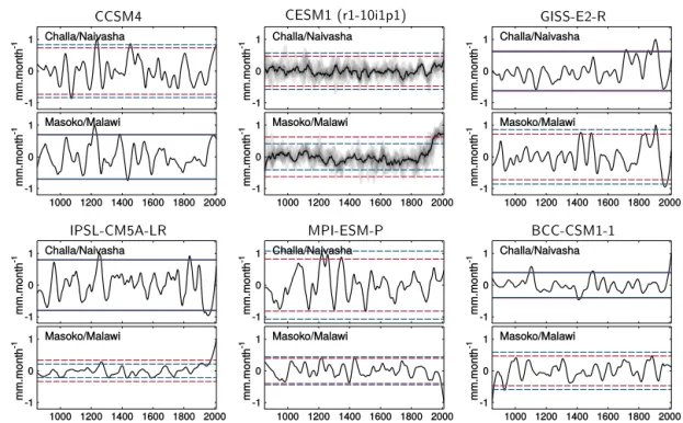
Figure 9.Simulated time series ofP_-E_{(black lines) over the Challa–Naivasha and Masoko–Malawi regions throughout the last millennium}

(850–2005). Results are mean annual values smoothed using a loess filter with a window of 100 years, and are presented as anomalies with respect to the entire period. The horizontal red lines are displayed on both sides of the zero line at two times standard deviation of the smoothed time series. The horizontal blue lines also represent 2 standard deviations on both sides of zero but based on the time series from pre-industrial control simulations. The horizontal lines are dashed if the variance of the simulation with time-varying forcing is significantly different (F_{test, considering a 5 % level) from the variance of the simulation with fixed forcing; if not, it is solid. For the CESM1 model, the}

black line is the median of the 10 ensemble members, while their range is shown in grey shading.

sults seem different, which raises the question whether ex-ternal forcing has any impact on the simulated hydroclimate. The lack of common timing among models in the simulated events actually suggests that the hydroclimate fluctuations are mostly or exclusively driven by internal variability.

5 The contribution of forced and internal variability

in simulated hydroclimate changes

5.1 Hydroclimate changes over the past millennium Whether the simulated East African hydroclimate results from internal variability or from changes in forcing is as-sessed in two steps: first by investigating potentially common signals among models, and second by comparing variability of the last-millennium hydroclimate changes against control simulations. In the previous section we suggested that little or no link can be established between last-millennium hydro-climate changes simulated by the different models. Indeed, if we first consider the Challa–Naivasha region, most correla-tions betweenP_-E_{time series simulated by different models} are not statistically significant and close to zero (Fig. 8). Ac-tually, the fact that there is no positive correlation between hydroclimate curves from different models does not neces-sarily mean that there is no impact of forcing in each model.

Indeed, the effect of changes in forcing may be different from one GCM to another, especially at the still relatively small spatial scale considered in this study.

In this regard, it is of interest to note that for the one model for which multiple ensemble members were available (CESM1), there is also no correlation between the differ-ent ensemble members that differ only in slightly differdiffer-ent air temperature at the start of the experiments (Otto-Bliesner et al., 2016). This means that the forced response has a much smaller magnitude than internal variability forP_-E _{in that} region, even at the multi-decadal timescale.

For the Masoko–Malawi region, the link between the hy-droclimate time series produced by different models is also low. However, most ensemble members of CESM1 show sig-nificantly positive correlations with each other, mainly due to a common increase inP_-E _{around 1800. This suggests} an impact, although limited, of external forcing on Masoko– Malawi hydroclimate during the last two centuries, as sim-ulated by CESM1. For the other models, if a significant re-sponse to forcing is present, it is too different between them to be revealed by the correlation, except for IPSL-CM5A-LR which correlates positively with the ensemble members of CESM1.

(13)

0.4 0.3 0.2 0.1 0 0.1 0.2 0.3 0.4

(a)

Challa/Naivasha

region

CCSM4 CESM1 GISS-E2-R

(b

)

M

a

s

o

k

o

/M

a

la

w

i

re

g

io

n CCSM4 CESM1 GISS-E2-R

Figure 10.Pearson correlation coefficients between global SSTs and mean annual rainfall over the Challa–Naivasha(a)and Masoko–Malawi (b)regions, in climate models for the period 850–1850 AD. In areas overprinted by white circles the null hypothesis of no correlation can be rejected at the 5 % level.

the variability in these time series and in the pre-industrial control runs, represented by the±2 standard-deviation enve-lope. It shows that theP_-E_{variance simulated over the last} millennium is in most cases very similar to that of the control simulations. This indicates that the radiative changes from GHGs, solar variability and relatively short-lived volcanic ef-fects have little influence on the selected variables compared to internal variability. The only noticeable difference in these variances is found for Masoko–Malawi in two of the models, CEMS1 and IPSL-CM5A-LR, which both show a P_-E in-crease in recent time. The similarity of the variances ofP_-E in fixed and time-varying forcing experiments, along with the lack of common P_-E _{changes in the last-millennium} sim-ulations among models, obviates the possibility of general agreement with the proxy results, and suggests that any ap-parent proxy-model agreement for this time period and these regions is coincidental. To obtain more information on the processes driving the simulated hydroclimate changes over the last millennium, the next section deals with the stability of teleconnections at different frequencies, and with the im-pact of changes in forcing on those teleconnections.

5.2 The stability of large-scale teleconnections

Since East African hydroclimate fluctuations in models are mostly driven by rainfall (see Sect. 4.2), only rainfall is considered here. The modern-day large-scale teleconnections have already been studied in Sect. 3.3. Hence, the period con-sidered in this section is 850–1850 AD, which allows us to focus on the last millennium without the influence of anthro-pogenic forcing.

(14)

0.4 0.3 0.2 0.1 0 0.1 0.2 0.3 0.4

(a)

Challa/Naivasha

region

(b

)

M

a

s

o

k

o

/M

a

la

w

i

re

g

io

Figure 11. Pearson correlation coefficients between global SSTs and mean annual rainfall over the Challa–Naivasha(a)and Masoko– Malawi(b)regions, using thepre-industrial control runsof the climate models. Rainfall and SSTs are mean annual values smoothed using a loess filter with a window of 100 years. In areas overprinted by white circles the null hypothesis of no correlation can be rejected at the 5 % level.

Fig. 4a). The role of equatorial Pacific SSTs during the last millennium is less clear among models, with both positive and negative correlations depending on the model selected.

Patterns of correlations between simulated Masoko– Malawi rainfall and SSTs are more heterogeneous (Fig. 10b). CCSM4 and MPI-ESM-P show a comparable picture as with Challa–Naivasha rainfall, which is also the case for CESM1 but only for the Indian Ocean. GISS-E2-R and, to a lesser extent, IPSL-CM5A-LR show an opposite pattern, and BCC-CSM1-1 suggests almost no link between Masoko–Malawi rainfall and SSTs. For this region, the pre-industrial last-millennium teleconnections differ strongly from the recent ones in all models except CCSM4 and GISS-E2-R (Fig. 4b). For this pre-industrial last-millennium period, the effect of changes in forcing on inter-annual rainfall teleconnections appears to be weak, given the very similar results of the last millennium runs (Fig. 10) and of the pre-industrial con-trol runs for both regions (Fig. S3). It is thus likely that the difference in teleconnection patterns between the pre-industrial period and recent decades, observed in the mod-els GISS-E2-R, IPSL-CM5A-LR and BCC-CSM1-1, is due

(15)

0.4 0.3 0.2 0.1 0 0.1 0.2 0.3 0.4

(a)

Challa/Naivasha

region

(b

)

M

a

s

o

k

o

/M

a

la

w

i

re

g

io

Figure 12. Pearson correlation coefficients between global SSTs and mean annual rainfall over the Challa–Naivasha(a)and Masoko– Malawi(b)regions in climate models for the pre-industrial period 850–1850 AD. Rainfall and SSTs are mean annual values smoothed using a loess filter with a window of 100 years. In areas overprinted by white circles the null hypothesis of no correlation can be rejected at the 5 % level.

The patterns of correlations become completely differ-ent when considering the smoothed last millennium simu-lations with changes in forcing (Fig. 12). Most corresimu-lations are not significant and relatively weak. Interestingly, in the forced runs no Indian Ocean dipole is observed in most model results at this centennial timescale and, more gener-ally, there is substantial difference in modelled large-scale teleconnections between simulations with time-varying forc-ing (Fig. 12) or fixed forcforc-ing (Fig. 11). This suggests that, at the centennial timescale, the forcing is able to mask the weak correlations associated with natural variability through-out the pre-industrial portion of the last millennium (850– 1850 AD). Nevertheless, the response of the different models to the same forcing strongly varies. Some models are charac-terized by a very homogeneous pattern of correlation that can be both negative or positive, while some models show a more patchy pattern.

6 General discussion and conclusions

Our analysis of East Africa’s hydroclimate over the last millennium is based on recent observational data, lake-based proxy reconstructions and the results of six GCMs. When compared to recent observations (1979–2005), sim-ulations of all models represent the unimodal seasonality of precipitation characterizing the Masoko–Malawi spatial domain rather well. The bimodal seasonality characteriz-ing the Challa–Naivasha domain is generally less well cap-tured by the GCMs, with a systematic underestimation of the long rains and overestimation of the short rains. Model skill in simulating modern-day (i.e. observed) large-scale tele-connections between East African precipitation and tropical SSTs strongly varies among the GCMs, with MPI-ESM-P and CESM1 generally displaying the most consistent pat-terns.

(16)

dis-play a different rainfall seasonality and different large-scale teleconnections with ocean SSTs. Furthermore the lake-based proxy reconstructions from these two regions even show opposite moisture-balance changes during the second half of the last millennium, highlighting the strong spatial heterogeneity characterizing East African hydroclimate dy-namics. Comparing the simulated variable P_-E _{with the} available reconstructions, we found the contribution of rain-fall to be dominant relative to actual evaporation in both re-gions. Model results and reconstructions show a very differ-ent timing of hydroclimate fluctuations over the past mil-lennium. Furthermore, there is no common signal among the time series modelled by different GCMs. This suggests that simulatedP_-E_{in East Africa is largely driven by} inter-nal variability rather than by common forcing, at least un-til 1850 AD. After that, half of the GCMs used simulate a relatively clear, but model-specific, response to forcing. These results are in line with those of Coats et al. (2015) who showed, using approximately the same set of GCMs, that multi-decadal droughts in the North American South-west over the last millennium do not seem to be driven by ex-ternal forcing. Similar conclusions were also reached by Kel-ley et al. (2012) who used GCMs to investigate the possibil-ity that the late winter drying trend observed in the Mediter-ranean region could be explained by anthropogenic forcing. In contrast, Fallah and Cubasch (2015) suggested an impact of forcing on multi-decadal droughts in Asia over the last millennium, namely through alteration of atmosphere–ocean interactions. These contrasting results could mean that some regions are more sensitive to forcing than others.

At the inter-annual timescale, models show robust telecon-nections between mean annual Indian Ocean SSTs and rain-fall over the Challa–Naivasha region during the pre-industrial portion of the last millennium, with positive (negative) cor-relation in the western (eastern) half of the basin. The link between rainfall over the Masoko–Malawi region and SSTs is less clear among models. At this timescale, the effect of external forcing on large-scale teleconnections appears neg-ligible. Although most of the time it is not significant, the In-dian Ocean dipole is still present using time series smoothed to highlight centennial variations, but only in fixed-forcing simulations. When taking into account the last millennium forcing, the result is completely different, with relatively ho-mogeneous patterns of correlation between precipitation in both regions and tropical SSTs. This means that, although the correlation pattern between Challa–Naivasha rainfall and Indian Ocean SSTs remains relatively similar for both inter-annual and centennial timescales when only natural variabil-ity is present, it is overwhelmed by the effect of forcing at the centennial timescale. An interesting question is whether the forcing actually alters the dynamical link between East African rainfall and SSTs, or if it only masks it because of a different impact on continental rainfall and SSTs. Answer-ing this question is out of the scope of this study, but it is of interest for the interpretation of records used for

reconstruct-ing phenomena like the IOD. Indeed, if dynamical relation-ships are not stable when considering different timescales, a record calibrated in observations of the recent period may not be representative of the studied phenomena over longer timescales.

Analysing an ensemble of models was particularly useful here to test the robustness of the results. Additionally, using individual models that contain several ensemble members al-lows attributing the simulated change to internal variability or to forcing, which is crucial in the present context of cli-mate change in the vulnerable East African region. On the other hand, using multi-model mean results to study varia-tion in local hydroclimate during the last millennium should be avoided. It does not make sense to average hydroclimate time series which are mostly driven by internal variability, since this would only result in concealing already weak re-sponses.

7 Data availability

All model results used in this study are publicly available and can be obtained in the Program for Climate Model Diagnosis and Inter-comparison (PCMDI; http://pcmdi9.llnl.gov) and the Earth System Grid (www.earthsystemgrid.org) archives.

The Supplement related to this article is available online at doi:10.5194/cp-12-1499-2016-supplement.

Acknowledgements. This work is supported by the BRAIN-be programme of the Belgian Federal Science Policy Office (BelSPO) through project BR/121/A2 “Patterns and mechanisms of climate extremes in East Africa” (PAMEXEA). We acknowledge the World Climate Research Programme’s Working Group on Coupled Modelling, which is responsible for CMIP, and we thank the climate modelling groups (listed in Table 1 of this paper) for producing and making available their model output. For CMIP the US Department of Energy’s Program for Climate Model Diagnosis and Intercomparison provides coordinating support and led development of software infrastructure in partnership with the Global Organization for Earth System Science Portals. Hugues Goosse is research director with the FRS/FNRS, Belgium.

Edited by: D. Fleitmann

Reviewed by: two anonymous referees

References

(17)

Anchukaitis, K. J. and Tierney, J. E.: Identifying coherent spa-tiotemporal modes in time-uncertain proxy paleoclimate records, Clim. Dynam., 41, 1291–1306, doi:10.1007/s00382-012-1483-0, 2012.

Anyah, R. O. and Qiu, W.: Characteristic 20th and 21st century precipitation and temperature patterns and changes over the Greater Horn of Africa, International J. Climatol., 32, 347–363, doi:10.1002/joc.2270, 2012.

Becht, R. and Harper, D. M.: Towards an understanding of human impact upon the hydrology of Lake Naivasha , Kenya, Hydrobi-ologia, 488, 1–11, 2002.

Berger, A.: Long-term variations of daily insolation and Quaternary climatic changes, Journal of the Atmo-spheric Sciences, 35, 2363–2367, doi:10.1175/1520-0469(1978)035<2362:LTVODI>2.0.CO;2, 1978.

Brown, E. T. and Johnson, T. C.: Coherence between trop-ical East African and South American records of the Little Ice Age, Geochem. Geophy. Geosy., 6, 1–11, doi:10.1029/2005GC000959, 2005.

Buckles, L. K., Verschuren, D., Weijers, J. W. H., Cocquyt, C., Blaauw, M., and Sinninghe Damsté, J. S.: Interannual and (multi-)decadal variability in the sedimentary BIT index of Lake Challa, East Africa, over the past 2200 years: assessment of the precipita-tion proxy, Clim. Past, 12, 1243–1262, doi:10.5194/cp-12-1243-2016, 2016.

Chen, M., Xie, P., Janowiak, J. E., and Arkin, P. A.: Global Land Precipitation: A 50-yr Monthly Analysis Based on Gauge Ob-servations, J. Hydrometeorol., 3, 249–266, doi:10.1175/1525-7541(2002)003>0249:GLPAYM>2.0.CO;2, 2002.

Clark, C., Webster, P., and Cole, J.: Interdecadal variability of the relationship between the Indian Ocean zonal mode and East African coastal rainfall anomalies, J. Climate, 16, 548–554, doi:10.1175/1520-0442(2003)016<0548:IVOTRB>2.0.CO;2, 2003.

Coats, S., Smerdon, J. E., Cook, B. I., and Seager, R.: Are Simu-lated Megadroughts in the North American Southwest Forced?*, J. Climate, 28, 124–142, doi:10.1175/JCLI-D-14-00071.1, 2015. Conway, D., Hanson, C. E., Doherty, R., and Persechino, A.: GCM simulations of the Indian Ocean dipole influence on East African rainfall: Present and future, Geophys. Res. Lett., 34, L03705, doi:10.1029/2006GL027597, 2007.

Cook, K. H. and Vizy, E. K.: Projected changes in east african rainy seasons, J. Climate, 26, 5931–5948, doi:10.1175/JCLI-D-12-00455.1, 2013.

Crowley, T. J. and Unterman, M. B.: Technical details concern-ing development of a 1200 yr proxy index for global volcanism, Earth Syst. Sci. Data, 5, 187–197, doi:10.5194/essd-5-187-2013, 2013.

Dinku, T., Ceccato, P., Grover-Kopec, E., Lemma, M., Connor, S. J., and Ropelewski, C. F.: Validation of satellite rainfall products over East Africa’s complex topography, Int. J. Remote Sens., 28, 1503–1526, doi:10.1080/01431160600954688, 2007.

Dufresne, J. L., Foujols, M. A., Denvil, S., Caubel, A., Marti, O., Aumont, O., Balkanski, Y., Bekki, S., Bellenger, H., Benshila, R., Bony, S., Bopp, L., Braconnot, P., Brockmann, P., Cadule, P., Cheruy, F., Codron, F., Cozic, A., Cugnet, D., de Noblet, N., Duvel, J. P., Ethé, C., Fairhead, L., Fichefet, T., Flavoni, S., Friedlingstein, P., Grandpeix, J. Y., Guez, L., Guilyardi, E., Hauglustaine, D., Hourdin, F., Idelkadi, A., Ghattas, J.,

Jous-saume, S., Kageyama, M., Krinner, G., Labetoulle, S., Lahel-lec, A., Lefebvre, M. P., Lefevre, F., Levy, C., Li, Z. X., Lloyd, J., Lott, F., Madec, G., Mancip, M., Marchand, M., Masson, S., Meurdesoif, Y., Mignot, J., Musat, I., Parouty, S., Polcher, J., Rio, C., Schulz, M., Swingedouw, D., Szopa, S., Talandier, C., Terray, P., Viovy, N., and Vuichard, N.: Climate change projections us-ing the IPSL-CM5 Earth System Model: From CMIP3 to CMIP5, Clim. Dynam., 40, 2123–2165, doi:10.1007/s00382-012-1636-1, 2013.

Fallah, B. and Cubasch, U.: A comparison of model simulations of Asian mega-droughts during the past millennium with proxy re-constructions, Clim. Past, 11, 253–263, doi:10.5194/cp-11-253-2015, 2015.

Flückiger, J., Monnin, E., Stauffer, B., Schwander, J., Stocker, T. F., Chappellaz, J., Raynaud, D., and Barnola, J.-M.: High-resolution Holocene N2O ice core record and its

relation-ship with CH₄ and CO₂, Global Biogeochem. Cy., 16, 1010, doi:10.1029/2001GB001417, 2002.

Funk, C., Dettinger, M. D., Michaelsen, J. C., Verdin, J. P., Brown, M. E., Barlow, M., and Hoell, A.: Warming of the Indian Ocean threatens eastern and southern African food security but could be mitigated by agricultural development, P. Natl. Acad. Sci. USA, 105, 11081–11086, doi:10.1073/pnas.0708196105, 2008. Gao, C., Robock, A., and Ammann, C.: Volcanic forcing of

cli-mate over the past 1500 years: An improved ice core-based in-dex for climate models, J. Geophys. Res.-Atmos., 113, 1–15, doi:10.1029/2008JD010239, 2008.

Garcin, Y., Williamson, D., Taieb, M., Vincens, A., Mathé, P. E., and Majule, A.: Centennial to millennial changes in maar-lake de-position during the last 45,000 years in tropical Southern Africa (Lake Masoko, Tanzania), Palaeogeogr. Palaeocl., 239, 334–354, doi:10.1016/j.palaeo.2006.02.002, 2006.

Garcin, Y., Williamson, D., Bergonzini, L., Radakovitch, O., Vin-cens, A., Buchet, G., Guiot, J., Brewer, S., Mathé, P. E., and Majule, A.: Solar and anthropogenic imprints on Lake Masoko (southern Tanzania) during the last 500 years, J. Paleolimnol., 37, 475–490, doi:10.1007/s10933-006-9033-6, 2007.

Gent, P. R., Danabasoglu, G., Donner, L. J., Holland, M. M., Hunke, E. C., Jayne, S. R., Lawrence, D. M., Neale, R. B., Rasch, P. J., Vertenstein, M., Worley, P. H., Yang, Z.-L., and Zhang, M.: The Community Climate System Model Version 4, J. Climate, 24, 4973–4991, doi:10.1175/2011JCLI4083.1, 2011.

Goddard, L. and Graham, N. E.: Importance of the Indian Ocean for simulating rainfall anomalies over eastern and southern Africa, J. Geophys. Res., 104, 19099, doi:10.1029/1999JD900326, 1999. Hansen, J. and Sato, M.: Greenhouse gas growth

rates, P. Natl. Acad. Sci. USA, 101, 16109–16114, doi:10.1073/pnas.0406982101, 2004.

Hastenrath, S., Nicklis, A., and Greischar, L.: Atmospheric-hydrospheric mechanisms of climate anomalies in the western equatorial Indian Ocean, J. Geophys. Res., 96, 20219–20235, 1993.

Hillbruner, C. and Moloney, G.: When early warning is not enough-Lessons learned from the 2011 Somalia Famine, Global Food Security, 1, 20–28, doi:10.1016/j.gfs.2012.08.001, 2012. Hoell, A., Funk, C., and Barlow, M.: The regional forcing of

(18)

Huffman, G. J., Adler, R. F., Bolvin, D. T., and Gu, G.: Improving the global precipitation record: GPCP Version 2.1, Geophys. Res. Lett., 36, 1–5, doi:10.1029/2009GL040000, 2009.

Hurtt, G. C., Chini, L. P., Frolking, S., Betts, R. A., Feddema, J., Fis-cher, G., Fisk, J. P., Hibbard, K., Houghton, R. A., Janetos, A., Jones, C. D., Kindermann, G., Kinoshita, T., Klein Goldewijk, K., Riahi, K., Shevliakova, E., Smith, S., Stehfest, E., Thomson, A., Thornton, P., van Vuuren, D. P., and Wang, Y. P.: Harmo-nization of land-use scenarios for the period 1500–2100: 600 years of global gridded annual land-use transitions, wood har-vest, and resulting secondary lands, Climatic Change, 109, 117– 161, doi:10.1007/s10584-011-0153-2, 2011.

International Federation of Red Cross and Red Crescent Societies (IFRC): Disaster relief emergency fund (DREF) – Kenya : Floods 2012, Tech. rep., International Federation of Red Cross and Red Crescent Societies, 2013a.

IFRC: Emergency appeal – Kenya : Floods 2013, Tech. Rep. April 2013, International Federation of Red Cross and Red Crescent Societies, 2013b.

International Research Institute for Climate and Society (IRI): Emerging La Nina conditions in the equatorial Pacific: Notes for the Health Community, Tech. rep., The International Research Institute for Climate and Society, 2010.

Izumo, T., Lengaigne, M., Vialard, J., Luo, J.-J., Yamagata, T., and Madec, G.: Influence of Indian Ocean Dipole and Pacific recharge on following year’s El Nino: interdecadal robustness, Clim. Dynam., 42, 291–310, doi:10.1007/s00382-012-1628-1, 2014.

Japan Agency for Marine-Earth Science and Technology (JAM-STEC): Seasonal Prediction: ENSO forecast, Indian Ocean fore-cast, Regional forefore-cast, http://www.jamstec.go.jp/frcgc/research/ d1/iod/sintex_f1%_announcements_s.html.en, last access: 30 October 2015.

Johnson, T. C. and McCave, I. N.: Transport mechanism and paleo-climatic significance of terrigenous silt deposited in varved sedi-ments of an African rift lake, Limnol. Oceanogr., 53, 1622–1632, doi:10.4319/lo.2008.53.4.1622, 2008.

Kelley, C., Ting, M., Seager, R., and Kushnir, Y.: The relative con-tributions of radiative forcing and internal climate variability to the late 20th Century winter drying of the Mediterranean region, Clim. Dynam., 38, 2001–2015, doi:10.1007/s00382-011-1221-z, 2012.

Kennedy, J. J., A, R. N., Smith, R. O., Parker, D. E., and Saunby, M.: Reassessing biases and other uncertainties in sea surface temper-ature observations measured in situ since 1850: 1. Measurement and sampling uncertainties, J. Geophys. Res.-Atmos., 116, 1–13, doi:10.1029/2010JD015218, 2011a.

Kennedy, J. J., Rayner, N. A., Smith, R. O., Parker, D. E., and Saunby, M.: Reassessing biases and other uncertainties in sea surface temperature observations measured in situ since 1850: 2. Biases and homogenization, J. Geophys. Res.-Atmos., 116, 1– 22, doi:10.1029/2010JD015220, 2011b.

Kirtman, B., Power, S., Adedoyin, J., Boer, G., Bojariu, R., Camil-loni, I., Doblas-Reyes, F., Fiore, A., Kimoto, M., Meehl, G., Prather, M., Sarr, A., Schär, C., Sutton, R., van Oldenborgh, G., Vecchi, G., and Wang, H.: Near-term climate change: projections and predictability, in: Climate Change 2013: The Physical Sci-ence Basis, Contribution of Working Group I to the Fifth Assess-ment Report of the IntergovernAssess-mental Panel on Climate Change,

edited by: Stocker, T., Qin, D., Plattner, G.-K., Tignor, M., Allen, S., Boschung, J., Nauels, A., Xia, Y., Bex, V., and Midgl, P., Cam-bridge University Press, CamCam-bridge, United Kingdom and New York, NY, USA, 2013.

Klein, S., Soden, B., and Lau, N.: Remote sea surface temperature variations during ENSO: Evidence for a tropical atmospheric bridge, J. Climate, 12, 917–932, 10.1175/1520-0442(1999) 012<0917:RSSTVD>2.0.CO;2, 1999.

Klein Goldewijk, K. and van Drecht, G.: HYDE3: Current and historical population and land cover, in: Integrated Modelling of Global Environmental Change, An Overview of IMAGE 2.4, edited by: Bouwman, A. F., Kram, T., and Goldewijk, K. K., chap. 6, Netherlands Environmental Assessment Agency, Bilthoven, the Netherlands, 93–112, 2006.

Laîné, A., Nakamura, H., Nishii, K., and Miyasaka, T.: A diagnostic study of future evaporation changes projected in CMIP5 climate models, Clim. Dynam., 42, 2745–2761, doi:10.1007/s00382-014-2087-7, 2014.

Lamarque, J.-F., Bond, T. C., Eyring, V., Granier, C., Heil, A., Klimont, Z., Lee, D., Liousse, C., Mieville, A., Owen, B., Schultz, M. G., Shindell, D., Smith, S. J., Stehfest, E., Van Aar-denne, J., Cooper, O. R., Kainuma, M., Mahowald, N., Mc-Connell, J. R., Naik, V., Riahi, K., and van Vuuren, D. P.: His-torical (1850–2000) gridded anthropogenic and biomass burning emissions of reactive gases and aerosols: methodology and ap-plication, Atmos. Chem. Phys., 10, 7017–7039, doi:10.5194/acp-10-7017-2010, 2010.

L’Heureux, M. L., Lee, S., and Lyon, B.: Recent multidecadal strengthening of the Walker circulation across the tropical Pa-cific, Nature Climate Change, 3, 1–6, doi:10.1038/nclimate1840, 2013.

Lyon, B.: Seasonal Drought in the Greater Horn of Africa and Its Recent Increase during the March-May Long Rains, J. Climate, 27, 7953–7975, doi:10.1175/JCLI-D-13-00459.1, 2014. Lyon, B. and DeWitt, D. G.: A recent and abrupt decline in

the East African long rains, Geophys. Res. Lett., 39, 1–5, doi:10.1029/2011GL050337, 2012.

MacFarling Meure, C., Etheridge, D., Trudinger, C., Steele, P., Langenfelds, R., Van Ommen, T., Smith, A., and Elkins, J.: Law Dome CO2, CH4 and N2O ice core records

ex-tended to 2000 years BP, Geophys. Res. Lett., 33, 2000–2003, doi:10.1029/2006GL026152, 2006.

McHugh, M. J.: Multi-model trends in East African rainfall as-sociated with increased CO2, Geophys. Res. Lett., 32, 1–4,

doi:10.1029/2004GL021632, 2005.

Merrifield, M. A.: A Shift in Western Tropical Pacific Sea Level Trends during the 1990s, J. Climate, 24, 4126–4138, doi:10.1175/2011JCLI3932.1, 2011.

Mutai, C. and Ward, M.: East African rainfall and the trop-ical circulation/convection on intraseasonal to interannual timescales, J. Climate, 13, 3915–3939, doi:10.1175/1520-0442(2000)013<3915:EARATT>2.0.CO;2, 2000.

Nicholson, S.: A review of climate dynamics and climate variability in Eastern Africa, in: The Limnology, Climatology and Paleocli-matology of the East African Lakes, edited by: Johnson, T. C. and Odada, E. O., Gordon and Breach, 25–56, 1996.