Long term halocarbon observations from a~coastal and an inland site in Sabah, Malaysian Borneo

(1)

ACPD

14, 1919–1969, 2014

Long term halocarbon observations

A. D. Robinson et al.

Title Page

Abstract Introduction

Conclusions References

Tables Figures

◭ ◮

Back Close

Full Screen / Esc

Printer-friendly Version Interactive Discussion

Discussion

P

a

per

|

D

iscussion

P

a

per

|

Discussion

P

a

per

|

Discuss

ion

P

a

per

|

Atmos. Chem. Phys. Discuss., 14, 1919–1969, 2014 www.atmos-chem-phys-discuss.net/14/1919/2014/ doi:10.5194/acpd-14-1919-2014

Atmospheric Chemistry and Physics

Open Access

Discussions

This discussion paper is/has been under review for the journal Atmospheric Chemistry and Physics (ACP). Please refer to the corresponding final paper in ACP if available.

Long term halocarbon observations from

a coastal and an inland site in Sabah,

Malaysian Borneo

A. D. Robinson1, N. R. P. Harris1, M. J. Ashfold1,*, B. Gostlow1, N. J. Warwick1,2,

L. M. O’Brien1, E. J. Beardmore1, M. S. M. Nadzir3,**, S. M. Phang3, A. A. Samah3,

S. Ong4, H. E. Ung4, L. K. Peng5, S. E. Yong5, M. Mohamad5, and J. A. Pyle1,2

1

Department of Chemistry, University of Cambridge, Lensfield Road, Cambridge, CB2 1EW, UK

2

National Centre for Atmospheric Science, NCAS, UK

3

Institute of Ocean & Earth Sciences, University of Malaya, 50603 Kuala Lumpur, Malaysia

4

Global Satria Life Sciences Lab, TB 12188, Taman Megajaya Phase 3, 91000 Tawau, Sabah, Malaysia

5

Malaysian Meteorological Department, Ketua Stesen GAW Lembah Danum, Jabatan Meteorologi Malaysia Cawangan Sabah, Lapangan Terbang Wakuba Tawau, Peti Surat 60109, 91011 Tawau, Sabah, Malaysia

*

(2)

ACPD

14, 1919–1969, 2014

Title Page

Tables Figures

◭ ◮

Back Close

Full Screen / Esc

Discussion

P

a

per

|

D

iscussion

P

a

per

|

Discussion

P

a

per

|

Discuss

ion

P

a

per

|

**

now at: School of Environmental and Natural Resource Sciences, Faculty of Science and Technology, Universiti Kebangsaan Malaysia, 43600 Bangi, Selangor, Malaysia

Received: 13 December 2013 – Accepted: 18 December 2013 – Published: 21 January 2014

Correspondence to: A. D. Robinson (adr22@cam.ac.uk)

(3)

ACPD

14, 1919–1969, 2014

Title Page

Tables Figures

◭ ◮

Back Close

Full Screen / Esc

Discussion

P

a

per

|

D

iscussion

P

a

per

|

Discussion

P

a

per

|

Discuss

ion

P

a

per

|

Abstract

Short lived halocarbons are believed to have important sources in the tropics where rapid vertical transport could provide a significant source to the stratosphere. In this study, quasi-continuous measurements of short-lived halocarbons are reported for two tropical sites in Sabah (Malaysian Borneo), one coastal and one inland (rainforest).

5

We present the observations for C2Cl4, CHBr3, CH2Br∗2 (actually∼80 % CH2Br2 and

∼20 % CHBrCl2) and CH3I from November 2008 to January 2010 made using our

µDirac gas chromatographs with electron capture detection (GC-ECD). We focus on the first 15 months of observations, showing over one annual cycle for each compound and therefore adding significantly to the few limited-duration observational studies that

10

have been conducted thus far in southeast Asia. The main feature in the C2Cl4

be-haviour at both sites is its annual cycle with the winter months being influenced by northerly flow with higher concentrations, typical of the Northern Hemisphere, with the summer months influenced by southerly flow and lower concentrations representative

of the Southern Hemisphere. No such clear annual cycle is seen for CHBr3, CH2Br∗2

15

or CH₃I. The baseline values for CHBr₃ and CH₂Br∗

2 are similar at the coastal

(over-all median: CHBr3 1.7 ppt; CH2Br∗2 1.4 ppt) and inland sites (CHBr3 1.6 ppt, CH2Br∗2

1.1 ppt), but periods with elevated values are seen at the coast (overall 95th percentile:

CHBr₃ 4.4 ppt; CH₂Br∗₂ 1.9 ppt) presumably resulting from the stronger influence of

coastal emissions. Overall median bromine values from [CHBr3]+[CH2Br∗2] are 8.0 ppt

20

at the coast and 6.8 ppt inland. The median values reported here are largely consistent with other limited tropical data and imply that southeast Asia generally is not, as has been suggested, a hot-spot for emissions of these compounds. These baseline values are consistent with the most recent emissions found for southeast Asia using the

p-TOMCAT model. CH₃I, which is only observed at the coastal site, is the shortest-lived

25

(4)

ACPD

14, 1919–1969, 2014

Title Page

Tables Figures

◭ ◮

Back Close

Full Screen / Esc

Discussion

P

a

per

|

D

iscussion

P

a

per

|

Discussion

P

a

per

|

Discuss

ion

P

a

per

|

1 Introduction

Reactions involving halogen compounds play an important role in the chemistry of both the stratosphere (e.g. Molina and Rowland, 1974; Yung et al., 1980) and the troposphere (e.g. Read et al., 2008). The sources of halogens are many and varied with important anthropogenic and natural components for many compounds (Montzka and

5

Reimann, 2011). Total atmospheric bromine concentrations are generally dominated by the halons (compounds of only anthropogenic origin widely used for fire control) and

CH3Br (used in agriculture, but with many sources). Their atmospheric concentrations

are well known and their lifetimes long enough to know with reasonable accuracy how much of these gases reaches the stratosphere. It was thus puzzling to find that they

10

could only account for 70–80 % of the bromine observed in the stratosphere (Wamsley et al., 1998; Dorf et al., 2006) though there remains uncertainty as to whether the discrepancy is that large (Kreycy et al., 2013).

Since there are no other known long-lived sources, the finger of suspicion points to

the shorter-lived CHBr3 and CH2Br2 which are observed in high concentration in the

15

marine boundary layer and are naturally produced in the surface ocean (e.g. Yokouchi et al., 2005; Butler et al., 2007; Zhou et al., 2008; O’Brien et al., 2009). For these compounds to be the source of the missing 20–30 % of the stratospheric bromine budget, they (or their breakdown products) have to be rapidly transported up to the stratosphere. The only credible place for this to occur is at low latitudes where upward

20

transport can be very rapid in the intense tropical convection. This possibility has been

investigated in a number of measurement (Schauffler et al., 1999; Laube et al., 2008;

Park et al., 2010; Brinckmann et al., 2012) and modelling (Levine et al., 2007, 2008; Aschmann et al., 2009; Hosking et al., 2010; Hossaini et al., 2010, 2012, 2013) studies. On balance it seems likely that the short-lived bromocarbons are responsible for the

25

apparent deficit.

(5)

ACPD

14, 1919–1969, 2014

Title Page

Tables Figures

◭ ◮

Back Close

Full Screen / Esc

Discussion

P

a

per

|

D

iscussion

P

a

per

|

Discussion

P

a

per

|

Discuss

ion

P

a

per

|

of reported tropical boundary layer measurements have been made using whole air samplers or short-term deployments of GC systems (Yokouchi et al., 2005; O’Brien et al., 2009; Pyle et al., 2011), or ship-borne measurements made during research cruises (Butler et al., 2007; Carpenter et al., 2009; Quack et al., 2004, 2007; Yokouchi et al., 1997; Nadzir et al., 2013; Brinckmann et al., 2012). No long-term and continuous

5

measurements in the tropics have been reported to date.

Accordingly, we have set up a small network of instruments to make continuous measurements at a number of sites in the West Pacific/southeast Asian region. This region was chosen as it is where convection is strongest, especially during NH win-ter (e.g. Newell and Gould-Stewart, 1981; Gettelman et al., 2002; Fueglistaler et al.,

10

2009). In addition, an early model study suggested high CHBr₃ emissions and

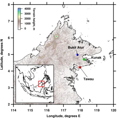
atmo-spheric concentrations here, due to the many islands and therefore large length of coastlines found in this region (Warwick et al., 2006), although this estimate has since been revised downward (Pyle et al., 2011). The first two instruments were installed in 2008 in the State of Sabah in Malaysian Borneo, one at a coastal site and one

in-15

land (Fig. 1). Early measurements were reported in Pyle et al. (2011). Here we report measurements from the subsequent years focussing on the period from late 2008 to

early 2010. In addition to CHBr3 and CH2Br∗2, we report our observations of C2Cl4,

a manufactured compound which we use to identify air with anthropogenic influence,

and CH₃I, a compound produced naturally in the ocean which has a short atmospheric

20

lifetime (7 days, Montzka and Reimann, 2011).

In Sect. 2 we describe the instruments used in this study, their calibration and the measurement quality reported here. Section 3 contains a discussion of the measure-ment sites including their physical characteristics, while in Sect. 4 we describe the modelling tools (NAME, p-TOMCAT) used in the interpretation of the data. The

mea-25

surements for C₂Cl₄, CHBr₃, CH₂Br∗

2and CH3I are presented in Sect. 5, with particular

(6)

ACPD

14, 1919–1969, 2014

Title Page

Tables Figures

◭ ◮

Back Close

Full Screen / Esc

Discussion

P

a

per

|

D

iscussion

P

a

per

|

Discussion

P

a

per

|

Discuss

ion

P

a

per

|

organic bromine in short-lived bromocarbons at each site. Finally, Sect. 6 summarises our findings and ongoing/future work.

2 Methodology

In Sect. 2.1 we briefly describe the instruments used for this work and discuss how we monitored instrument performance throughout the deployment. In Sect. 2.2 we discuss

5

the calibration methodology used for each instrument.

2.1 Instrument

The instruments used for these observations were the original µDirac gas chro-matographs built by us for use on balloons, with electron capture detection (GC-ECD), in a modified configuration appropriate for extended ground-based deployment

10

as described in Pyle et al. (2011). The instrument is described in detail in Gostlow et al. (2010). Briefly, each sample is pre-concentrated using a Carboxen trap. The trap is then heated and the gaseous constituents are separated on a 10 m long, 0.18 mm i.d. capillary column (Restek MXT 502.2) prior to measurement in the ECD. As the in-struments are designed to run unattended, the control software runs chromatograms

15

according to a pre-determined sequence of samples bracketed by calibration and blank chromatograms. The sequence includes frequent calibrations using the same volume as the samples (20 mL) for correction of instrument sensitivity drift and precision

deter-mination. The sequence also runs calibrations at a range of different volumes so that

instrument response curves are generated for each target compound to allow for

non-20

linearity. The response curves are fit using a third order polynomial. Chromatograms and system data are stored on a host computer for later analysis using in-house soft-ware to determine peak heights for the target compounds which are then converted into mixing ratios by comparison with the calibration standards. Mixing ratios are reported as dry air mole fraction in ppt.

(7)

ACPD

14, 1919–1969, 2014

Title Page

Tables Figures

◭ ◮

Back Close

Full Screen / Esc

Discussion

P

a

per

|

D

iscussion

P

a

per

|

Discussion

P

a

per

|

Discuss

ion

P

a

per

|

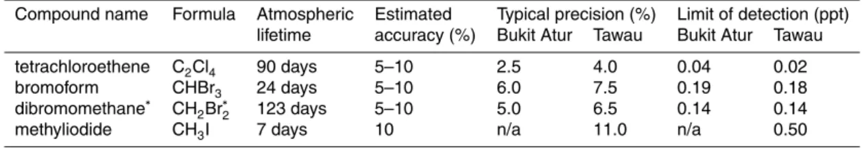
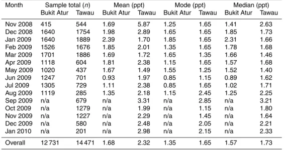
Measurement performance is monitored for each target compound during the anal-ysis of the chromatograms, and the typical performance for the measurement period

reported here is summarised in Table 1. For C2Cl4 the typical measurement precision

(1 s.d.) is 2.5 % and 4.0 % at Bukit Atur and Tawau respectively. The typical

measure-ment precision of CHBr3is 6.0 % and 7.5 % at Bukit Atur and Danum respectively and

5

those for CH2Br∗2 are 5.0 % and 6.5 %. Sample concentrations for C2Cl4, CHBr3 and

CH₂Br∗₂ are always above the limit of detection at both sites. CH₃I is only measured

at Tawau (the µDirac at Bukit Atur did not achieve satisfactory chromatographic

sep-aration for reliable quantification) and the typical precision is 11 %. The CH3I peak is

small in the sample chromatograms so particular care is taken in assessing its signal

10

to noise ratio (SNR). The SNR varies over time depending on the instrument condition and environment, and is calculated separately for each analysis period (typically 1–2 weeks) for which concentrations are calculated. Between January and June 2009, the estimated detection limit (defined using a SNR of 10) decreases from 0.9 ppt to 0.3 ppt as a result of reduced noise in the chromatograms and for the rest of 2009 it is below

15

0.2 ppt.

The chromatographic set-up uses a 10 m column for these measurements and this

provides a good separation for C2Cl4and CHBr3. However, the CH2Br2peak co-elutes

with that of CHBrCl2 with a 10 m column and so we report a combined value called

CH₂Br∗

2which we estimate to be 10–30 % higher than the CH2Br2value alone (O’Brien

20

et al., 2009). This co-elution problem is further discussed in Gostlow et al. (2010). In a recently improved version of the instrument where a 20 m long column is used, these two compounds are partly separated and so individual values can be derived by

peak fitting using two Gaussian fits. These new measurements of CH2Br2and CHBrCl2

using a 20 m column in similar tropical locations shows the ratio (10–30 %) to be still

25

valid, as in O’Brien et al. (2009).

The instrument based at the coastal site developed a problem with desorption ef-ficiency caused by incomplete thermal desorption of the target molecules from the

adsorbent. This affected the quantification of the CH₂Br∗

(8)

ACPD

14, 1919–1969, 2014

Title Page

Tables Figures

◭ ◮

Back Close

Full Screen / Esc

Discussion

P

a

per

|

D

iscussion

P

a

per

|

Discussion

P

a

per

|

Discuss

ion

P

a

per

|

chromatogram to the next. However, we are still able to use calibration chromatograms

for CH₂Br₂ as these are preceded by a blank chromatogram. About one in every ten

sample chromatograms is also usable for the CH2Br∗2peak as these are also preceded

by a blank. As a result of this problem CH2Br∗2 is only reported for about 1 in every

10 samples at Tawau. The C₂Cl₄and CHBr₃ peaks are not affected by this problem at

5

Tawau as these molecules are always completely retained on the lighter Carboxen at the front of the adsorbent bed.

2.2 Calibration

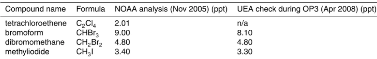
Samples are calibrated by running frequent chromatograms using background air spiked with key target compounds. The cylinders (one for each instrument) are

sup-10

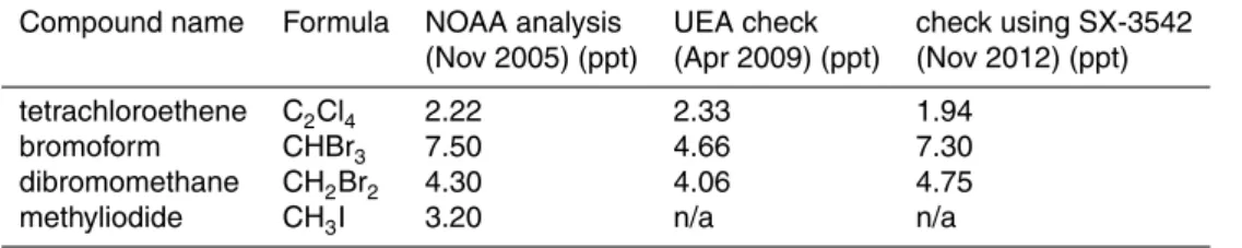
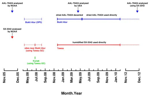
plied by the Earth System Research Laboratory (ESRL) within the National Oceanic and Atmospheric Administration (NOAA) so that the reported mixing ratios are linked directly to the NOAA halocarbon calibration scales. Figure 2 summarises the period of data coverage for this study together with a time-line of the calibration cylinders in use at the two sites. The calibration gas in use at Tawau for the entire period of this

15

study is in a high quality, humidified stainless steel cylinder (Essex Cryogenics Inc., cylinder SX-3542). The composition of this cylinder for the four compounds of interest is reasonably stable (Table 2a) and we plan to send this cylinder back to NOAA for subsequent analysis. The calibration gas in use at Bukit Atur from November 2008 to May 2009 was decanted into a 36 L stainless steel electropolished flask from a dried

20

NOAA Aculife cylinder (AAL-70424) in October 2008. Comparisons of this decanted cylinder with the Aculife cylinder at either end of this period reveal a significant change

for CH2Br2and CHBr3 and a smaller one in C2Cl4(Table 2b). The agreement with the

Aculife standard is much better in the later comparison which was performed in Sabah under the same conditions as the atmospheric measurements. We do not know why

25

the first comparison should have been poor (it was done in Cambridge just prior to shipping) though we suspect it is related to temporary adsorption on the canister walls.

(9)

ACPD

14, 1919–1969, 2014

Title Page

Tables Figures

◭ ◮

Back Close

Full Screen / Esc

Discussion

P

a

per

|

D

iscussion

P

a

per

|

Discussion

P

a

per

|

Discuss

ion

P

a

per

|

CH2Br∗2 at Tawau and Bukit Atur (Sect. 5.1) using the values derived in the second

comparison (last column of Table 2b), we choose to use this for the final analysis, rather than the values from the October 2008 check (or an average of the two checks). From May 2009 the NOAA Aculife cylinder (AAL-70424) used for the decanting is used directly at Bukit Atur. This cylinder appears to be more stable than the decanted

cylin-5

der though not as stable as the SX-3542 cylinder in use at Tawau (Table 2c). For the analysis of our Bukit Atur data from May 2009 to January 2010 we use the values from the check against the University of East Anglia (UEA) made in April 2009 using their NOAA SX cylinder, as this is closest in time to the period of the measurements. We also have more confidence in the comparison made at UEA (April 2009) under stable

10

laboratory conditions using their GC-MS than in an incomplete comparison made at Bukit Atur (November 2012) over 3 yr later. During June and July 2008 our measure-ments at Bukit Atur, analysed using the same NOAA (SX-3542) standard (later used at Tawau), compared well with GC-MS measurements made by UEA (Gostlow et al., 2010; Pyle et al., 2011).

15

In addition, we took part in an inter-comparison of measurements by several labora-tories using a round robin NOAA calibration standard (Jones et al., 2011). This showed our laboratory calibration scale to be within the instrumental error (10–20 %, 2 sigma) of this new NOAA standard. In July 2008 we ran our two instruments side-by-side at

Bukit Atur, measuring C2Cl4, CHBr3 and CH2Br∗2 in ambient air, using the same

cali-20

bration gas on both GC-ECDs. For this 4 day period we found that the observations of

C₂Cl₄, CHBr₃and CH₂Br∗

2from the two instruments were within 6 %, 1 % and 15 % of

each other respectively.

3 Field deployment

We have been making halocarbon observations in Sabah (Malaysian Borneo) since

25

(10)

ACPD

14, 1919–1969, 2014

Title Page

Tables Figures

◭ ◮

Back Close

Full Screen / Esc

Discussion

P

a

per

|

D

iscussion

P

a

per

|

Discussion

P

a

per

|

Discuss

ion

P

a

per

|

a southeast Asian tropical rainforest), Hewitt et al. (2010). Two µDirac GCs were used in OP3: one was based at the Global Atmospheric Watch (GAW) station at Bukit Atur (Gostlow et al., 2010) and the other made “mobile” measurements at several rainforest locations in Danum Valley and during a 4 day visit to the coast at Kunak (Pyle et al., 2011). At the end of the OP3 campaign the µDirac GC at the Bukit Atur GAW

5

station was left running and the second “mobile” instrument was moved to a coastal site near Tawau where it remained for the period of this study. The instrument at Bukit

Atur is visited at ∼2 weeks intervals (and on request) by staff from the Malaysian

Meterological Department (MMD) who manage the site. The Tawau instrument was

visited at∼1 month intervals and on request by one of our collaborators from Global

10

Satria Sdn. Bhd. (an aquaculture company). Neither instrument was connected to the internet so these visits were essential for data recovery and monitoring of instrument performance. Periodic service visits (every 9–12 months) were made to both sites by

Cambridge University sta_ff. As a result of this low intensity monitoring, the performance

of the instruments varies over time depending on the condition of the instrument and

15

its environment. Each site is now described in the following sub-sections.

3.1 Danum Valley rainforest site: the Bukit Atur GAW station

The Danum Valley conservation area covers 438 km2and is one of the largest, most

im-portant and best-protected expanses of pristine lowland dipterocarp rainforest

remain-ing in southeast Asia. The GAW station located on Bukit Atur (4.980◦N, 117.844◦E,

el-20

evation 426 m) has been in operation since 2004 and is reasonably remote being∼50

linear km away from the nearest town of Lahad Datu (Fig. 1). The station is equipped with a range of monitoring instruments and an automatic weather station located on a 5 m roof-top platform. The 100 m tower, which adjoins the laboratory, has air-intakes and platforms for sampling equipment at various levels and is the tallest instrumented

25

(11)

ACPD

14, 1919–1969, 2014

Title Page

Tables Figures

◭ ◮

Back Close

Full Screen / Esc

Discussion

P

a

per

|

D

iscussion

P

a

per

|

Discussion

P

a

per

|

Discuss

ion

P

a

per

|

physical properties), reactive gases (filterpack sampling), persistent organic pollutants, solar radiation and meteorological parameters. The site is operated by the Malaysian

Meteorological Department (MMD) and staff visit weekly from their nearest office at

Tawau airport. The station itself is located on a hill-top∼200 m above the valley floor

and the inlet for the µDirac instrument is attached 12 m up the tower, several meters

5

above the roof of the site building. The instrument is placed in an air-conditioned room in the main GAW building. The topography in the area consists of a series of hills

∼400 m a.s.l. with valley floors down to∼200 m a.s.l.. One of the largest mountains in

the area is Mount Danum at 1093 m a.s.l. The rainforest extends to all areas including mountain tops. Primary unlogged rainforest in the conservation area is surrounded by

10

areas of secondary rainforest (which have been logged in recent years). In terms of site meteorology, a clear diurnal cycle in rainfall is observed at the nearby Danum Val-ley Field Centre (DVFC) with an afternoon peak around 15:00 LT resulting from diurnal development of convective cells following the midday peak in temperature (Hewitt at al., 2010). Boundary layer stability also varies diurnally from highly stable at night

(of-15

ten leading to dense fog at night) to highly unstable during the day due to the onset of strong convection coupled with low wind speeds (Pearson et al., 2010).

3.2 Tawau coastal site: kampung Batu Payong

The Tawau coastal site is located in the peaceful village of Kampung Batu Payong

(4.223◦N, 117.997◦E, elevation 15 m) and is∼10 km from Tawau centre and∼85 km

20

south of the Bukit Atur rainforest station (Fig. 1). Between July 2008 and October 2011 the µDirac instrument here was located in an air-conditioned room at a fish hatchery site maintained by the Global Satria company. There are no seaweed beds in the im-mediate vicinity of the site. The activity at the site does not involve the use of any seaweeds (which are known to emit bromocarbons) and we do not find any evidence

25

of emissions from the hatchery activities. The air inlet is located∼5 m a.g.l. at the site

(about roof-top height) 40 m away from the shoreline. There is an unobstructed view

(12)

ACPD

14, 1919–1969, 2014

Title Page

Tables Figures

◭ ◮

Back Close

Full Screen / Esc

Discussion

P

a

per

|

D

iscussion

P

a

per

|

Discussion

P

a

per

|

Discuss

ion

P

a

per

|

at the foot of a small group of hills extending to the north, reaching an elevation of 350 m. A low cost weather station at the site gives an indication of wind speed and direction, temperature and humidity. This reveals a typical diurnal variation in wind due to land/sea breezes expected for coastal sites, though this does not obviously influence the observations reported here.

5

4 Models

Two modeling tools are used in this paper to assist in the interpretation of the observa-tions. They are now described in turn in Sects. 4.1 and 4.2.

4.1 NAME

The Numerical Atmospheric dispersion Modelling Environment (NAME) is a

La-10

grangian particle dispersion model developed by the UK Met Office (e.g. Jones et al.,

2007), which has been extensively used for analysis of long-term halocarbon data sets (e.g. Manning et al., 2003; Simmonds et al., 2006; Derwent et al., 2007). Abstract

par-ticles are moved through the model atmosphere by a combination of 0.5625◦_longitude

by 0.375◦ latitude mean wind fields calculated by the UK Met Office Unified Model

15

(Davies et al., 2005), and a random walk turbulence scheme. NAME can be run back-wards in time, to see where the air measured at a particular site may have originated, and forwards to see where air from a particular emission source might go. Each of these capabilities have previously been used to investigate relationships between sources, transport and measurements of pollutants (e.g. Redington and Derwent, 2002; Witham

20

and Manning, 2007).

Here, NAME is run backwards in time to reveal the origin of air arriving at Bukit Atur and Tawau. For each 3 h period thousands of inert particles (carrying an arbitrary mass) are released and travel backwards in time for 12 days. At each 15 min time-step the location of each particle is recorded. Then, at the end of the run this information

(13)

ACPD

14, 1919–1969, 2014

Title Page

Tables Figures

◭ ◮

Back Close

Full Screen / Esc

Discussion

P

a

per

|

D

iscussion

P

a

per

|

Discussion

P

a

per

|

Discuss

ion

P

a

per

|

is used to create an “air history map”. Here, we only record near surface particles (lowest 100 m of the model) which indicate where air may have been exposed to surface emissions. Monthly mean air histories are then calculated. The air history maps made for Tawau are almost identical to those from Bukit Atur so are not shown here.

4.2 p-TOMCAT

5

The global chemistry transport model (CTM), p-TOMCAT, is used to analyse the causes of seasonal bromoform variability at Bukit Atur. The basic formulation of p-TOMCAT is described in Cook et al. (2007) and Hamilton et al. (2008). Tracer transport is based on 6 hourly meteorological fields, including winds and temperatures, derived from Euro-pean Centre for Medium-Range Weather Forecasts operational analysis for the years

10

2008, 2009 and 2010. Here we use a high resolution (0.5◦×0.5◦) version with

bromo-form tracers “coloured” according to the region of emission and simple OH oxidation chemistry, described previously in Pyle et al. (2011) and Warwick et al. (2006). The degradation of bromoform is determined using 3-D fields of pre-calculated hourly OH values taken from a previous p-TOMCAT integration and photolysis frequencies from

15

an integration of the Cambridge 2-D model using cross section data summarised by Sander et al. (2003). For further details see Pyle et al. (2011). Here we compare time series of bromoform from the model output with the measurements.

5 Results and discussion

In this section we present the measurements of C₂Cl₄, CHBr₃ and CH₂Br∗₂from both

20

sites and CH3I from Tawau only. We first show that C2Cl4 can be used as a good

tracer of air mass, differentiating clearly between air masses with anthropogenic and

unpolluted origins. This provides a valuable background for the analysis of the three,

primarily biogenic, short-lived compounds, CHBr3, CH2Br∗2 and CH3I. In this section

we also assess the total organic Br coming from CHBr3 and CH2Br∗2 combined. We

(14)

ACPD

14, 1919–1969, 2014

Title Page

Tables Figures

◭ ◮

Back Close

Full Screen / Esc

Discussion

P

a

per

|

D

iscussion

P

a

per

|

Discussion

P

a

per

|

Discuss

ion

P

a

per

|

discuss the implications of these observations, in particular for the regional emissions

of CHBr3and CH2Br∗2.

5.1 Perchloroethene

Perchloroethene (C2Cl4) is an excellent anthropogenic tracer with few (if any) known

natural sources. Its main anthropogenic sources are the textile industry, dry-cleaning

5

applications and in vapour degreasing of metals (Montzka and Reimann, 2011). It currently has a Northern Hemisphere background concentration of 2–5 ppt with a pronounced seasonal variation, likely due to variation in the concentration of its major sink, the OH radical. In the Southern Hemisphere the background concen-tration is lower (0.5–1 ppt), though still with a pronounced seasonal variation (see

10

http://agage.eas.gatech.edu/data.htm; Simmonds et al., 2006). C₂Cl₄has an estimated

lifetime of∼90 days (see Table 1–4 in Montzka and Reimann, 2011), making it a good

tracer for studying long range transport.

At Bukit Atur and Tawau the C₂Cl₄ dry air mole fractions ranged typically from

0.3–0.8 ppt in May–August 2009 to 1.0–3.7 ppt from November 2008 to March 2009

15

(Fig. 3a). “Above baseline” spikes are observed occasionally at Tawau, but for most of the time the data at Bukit Atur and Tawau track each other on monthly and daily

timescales. As the two sites are 85 km apart and as both C₂Cl₄time series track each

other closely, it seems there is little local contribution from Sabah to the background mixing ratio.

20

For the 4 month period between December 2008 and March 2009 there is a

system-atic difference in the C2Cl4observations at the two sites, with the observations at Bukit

Atur on average 48 % higher than those at Tawau. It is surprising to find this large

sys-tematic di_fference given that the observations of C₂Cl₄ were within 6 % of each other

when the GCs ran side-by-side at the same site and with the same calibration gas at

25

Bukit Atur in July 2008 (Sect. 2 last paragraph). The differences are probably due to

(15)

ACPD

14, 1919–1969, 2014

Title Page

Tables Figures

◭ ◮

Back Close

Full Screen / Esc

Discussion

P

a

per

|

D

iscussion

P

a

per

|

Discussion

P

a

per

|

Discuss

ion

P

a

per

|

at Bukit Atur between November 2008 and May 2009 and therefore we have more confidence in the time series from Tawau (see Sect. 2.2).

Although there is a greater frequency of high (local pollution) spikes at Tawau these do not impact significantly on the underlying background which is similar to that at Bukit Atur. The seasonal trend at both sites is clear from box and whisker

5

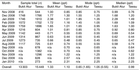
plots (Fig. 4a and d) and the tabulated monthly mean, median and modal values (Ta-ble 3a) which show low levels and low variability in the Northern Hemisphere summer

months in contrast with higher levels in winter. To further explore these seasonal diff

er-ences and site-to-site similarities, for selected months we use probability distributions

from the C₂Cl₄ observations, using a size interval of 0.1 ppt (Fig. 5a and e). In

Jan-10

uary/February 2009 there is a broad distribution of mixing ratios at both sites ranging from 0.85 to 3.75 ppt, tailing towards higher mixing ratios. The Tawau coastal median value in January/February 2009 (seen in Fig. 5a) is lower (1.30 ppt) than that inland at Bukit Atur (1.91 ppt). In June/July 2009 the distribution at each site has a much nar-rower range (0.25 to 1.65 ppt) and the median values are similar, though the coastal

15

median (0.45 ppt) is still lower than inland (0.63 ppt). In January/February 2009 the Bukit Atur instrument ran on the decanted calibration air from the NOAA Aculife cylinder AAL-70424, whereas in June/July 2009 the calibration came directly from the Aculife cylinder.

The seasonal changes in C₂Cl₄ are linked to changes in the prevailing monsoon

20

flow, and the inter-hemispheric gradient typically observed for gases with predomi-nantly Northern Hemisphere anthropogenic sources. Air history maps generated using NAME are used here to illustrate the seasonal changes in transport. From the months of November through to February the air mass history is influenced strongly by air com-ing from the north and east (Fig. 6a, January 2009). The large urban centres in and

25

around China in this region are expected to contribute to the background level of C₂Cl₄

(16)

ACPD

14, 1919–1969, 2014

Title Page

Tables Figures

◭ ◮

Back Close

Full Screen / Esc

Discussion

P

a

per

|

D

iscussion

P

a

per

|

Discussion

P

a

per

|

Discuss

ion

P

a

per

|

the air mass history indicates that Sabah is influenced strongly from the region to the southeast, characterised by Southern Hemisphere air originating from the Indonesian islands and Northern Australia (Fig. 6c, June 2009). As there are no major sources

of C₂Cl₄ across this region and the air masses are not influenced by emission from

for example Jakarta, we find (as expected) background mixing ratios to be low.

Octo-5

ber sees a transition between background air influenced by the Southern Hemisphere and Northern Hemisphere air influenced by China and other large urban centres. It is thus an example of a transition period between the two monsoon regimes (Fig. 6d, October 2009).

5.2 Bromoform

10

Bromoform (CHBr3) is an excellent tracer of marine air and is an important source of

organic bromine to the atmosphere (Carpenter and Liss, 2000). An open ocean, phy-toplankton source has been identified (Tokarczyk and Moore, 1994), and macroalgae found in coastal areas are also well known as major sources of bromoform (Moore and Tokarczyk, 1993). Emission fluxes in coastal regions are thought to be higher than in

15

the open ocean (Quack and Wallace, 2003; Yokouchi et al., 2005; Butler et al., 2007) though the relative contribution from coasts and from the open ocean to the total global

emission remains uncertain. Recent estimates of the global emissions of CHBr3 are

in the range 430–1400 Gg Br yr−1(Liang et al., 2010; Pyle et al., 2011; Ordonez et al.,

2012 and Table 1–8 in Montzka and Reimann, 2011) though much lower estimates of

20

120 and 200 Gg Br yr−1are given by Ziska et al. (2013). Although bromoform emissions

are dominated by natural sources there are minor anthropogenic contributions from by-products of drinking water chlorination in the presence of bromide ions, salt water swim-ming pools and power plant cooling water (Worton et al., 2006). In the atmosphere,

CHBr3has a lifetime of 24 days (from Table 1–4 in Montzka and Reimann, 2011) which

25

(17)

ACPD

14, 1919–1969, 2014

Title Page

Tables Figures

◭ ◮

Back Close

Full Screen / Esc

Discussion

P

a

per

|

D

iscussion

P

a

per

|

Discussion

P

a

per

|

Discuss

ion

P

a

per

|

The background CHBr₃ concentration at both Bukit Atur and Tawau is broadly in

the range 0.5 to 3 ppt. In contrast to the time series of C2Cl4, there is no

unambigu-ous seasonal variation in the background CHBr3 concentration (Fig. 3b). During the

periods when we report CHBr₃ mixing ratios from both sites, the background

con-centrations are sometimes the same within experimental error (e.g. Fig. 5b for

Jan-5

uary/February 2009), and in some months the coastal background is higher than inland (e.g. Fig. 5f for June/July 2009). These probability distributions also indicate that we do not observe strong seasonality in the background mixing ratio at Tawau. In contrast, there is a suggestion of a seasonal cycle, with a Northern Hemisphere winter peak, in the data collected inland at Bukit Atur (e.g. Fig. 4b). To emphasise this point, the

10

median mixing ratios for the two sites were similar in January/February 2009 (1.67 ppt at Tawau and 2.04 ppt at Bukit Atur), whereas for June/July 2009 the median value for Tawau (1.68 ppt) was higher than at Bukit Atur (0.95 ppt). Clearly, measurements

over many years are needed to ascertain whether the somewhat di_fferent behaviour

we have observed at the two sites in Borneo is a persistent feature. See Table 3b for

15

the statistical summaries of all the relevant periods.

A major di_fference between the two sites is that there are frequent periods (spikes)

at Tawau when very high levels (>10 ppt) of bromoform are observed, whereas at

Bukit Atur such episodes are rare, and the highest concentration is just 5.5 ppt. This

di_fference in variability is shown clearly in the box and whisker plots for Bukit Atur and

20

Tawau (Fig. 4b and e) where CHBr3observations>10 ppt at Tawau are seen in 12 of

the 15 reported months.

Various factors determine the concentrations we observe at these two sites. The

sources of CHBr3are certainly heterogeneous in space, and so the mere fact that the

boundary layer is influenced by different regions in different seasons (Fig. 6) leads to

25

(18)

ACPD

14, 1919–1969, 2014

Title Page

Tables Figures

◭ ◮

Back Close

Full Screen / Esc

Discussion

P

a

per

|

D

iscussion

P

a

per

|

Discussion

P

a

per

|

Discuss

ion

P

a

per

|

For example, northeast Sabah and the archipelagos between Sabah and the Philip-pines are major seaweed farming areas whose output has grown quickly over the last 20 yr (Phang, 2006; Perez, 2011). At present it appears that entirely natural emissions of bromoform in the region are significantly larger than those linked to aquaculture (Leedham et al., 2013) but continued rapid growth in the cultivation of many species

5

with commercial potential (Goh and Lee, 2010; Tan et al., 2013) could change this sit-uation (Phang et al., 2010). Further, the strength of individual sources is likely to vary over time. In the case of seaweeds, it seems likely that their halocarbon emissions will depend on environmental factors such as temperature, rainfall, wind, sunlight and if applicable, the phase of the cropping cycle (Seh-Lin Keng et al., 2013; Leedham et al.,

10

2013 and references therein). Given this complexity, without extensive biological field

surveys it is difficult to explain much of the variability in detail.

However, we are able to examine how well the CTM p-TOMCAT is able to simulate the long-term statistical properties of observed bromoform mixing ratios. The model configuration is described in Sect. 4.2, and the bromoform emissions are those

devel-15

oped by Pyle et al. (2011) as an update to Warwick et al. (2006). These emissions provide the best match with our earlier observations collected at Bukit Atur during

OP3 (Pyle et al., 2011). The observed time series for CHBr3 is consistent with the

p-TOMCAT model output using the revised emission estimate as shown for Tawau in Fig. 7a. The model is unable to capture the very high values seen in the

observa-20

tions, which is to be expected given the model resolution and the uniform distribution of emissions around the coastlines in the model. The model does a reasonable job of reproducing the background observed concentration throughout 2009 at Tawau. The bromoform observations and model output for the four months from December 2008 to March 2009 are compared as a probability distribution in Fig. 7b. The

observa-25

(19)

ACPD

14, 1919–1969, 2014

Title Page

Tables Figures

◭ ◮

Back Close

Full Screen / Esc

Discussion

P

a

per

|

D

iscussion

P

a

per

|

Discussion

P

a

per

|

Discuss

ion

P

a

per

|

5.3 Dibromomethane

It is thought that the marine sources of dibromomethane (CH2Br2) are similar to those

of CHBr3, as shown by the strong correlations observed between their atmospheric

concentrations (Yokouchi et al., 2005; Carpenter et al., 2009). Emission fluxes are probably higher in coastal regions than over the open ocean (Ziska et al., 2013), but

5

the relative effect on coastal atmospheric measurements is less marked than for CHBr3

due to a longer lifetime for CH₂Br₂of∼120 days (Table 1–4 in Montzka and Reimann,

2011). The CH2Br2lifetime is expected to be slightly lower than 120 days in the tropics

due to the higher abundance of the OH radical. Open ocean sources are also more

important globally than coastal sources. Recent estimates of the global CH₂Br₂

emis-10

sions are 50–70 Gg Br yr−1(Liang et al., 2010; Ordonez et al., 2012).

The mixing ratios of CH2Br∗2measured at Bukit Atur and Tawau are shown in Fig. 3c.

The observed baseline values of between 1 and 2 ppt for CH2Br2* (remembering that

10–30 % of this could be CHBrCl₂) at the two sites are similar, as reflected in the

me-dian values in Table 3. The variability at Tawau is much less than for CHBr3. Statistically,

15

the observations at Bukit Atur and Tawau are similar to each other as shown by the box and whisker plots, although the two months at Tawau with distinctly low median val-ues (March/April 2009) are not reflected in the Bukit Atur observations (Fig. 4c and f).

There is a definite hint of some seasonality in the CH2Br∗2measurements (Fig. 5c and

g), though multi-year data are required to determine whether there is a seasonal cycle.

20

Median values in January/February 2009 are almost the same at both sites (1.20 and 1.28 ppt at Bukit Atur and Tawau respectively), though in June/July 2009 the median value at Tawau (1.33 ppt) is distinctly higher than at Bukit Atur (1.00 ppt).

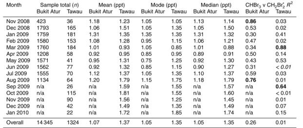
We find that in all reported months at Bukit Atur there is always a positive correlation

between the observations of CH2Br∗2 and CHBr3, suggesting a common source

(Ta-25

ble 3c). Nadzir et al. (2013) also found a strong positive correlation between CHBr₃and

CH2Br2in whole air flask samples taken during a 2009 cruise in the South China and

(20)

ACPD

14, 1919–1969, 2014

Title Page

Tables Figures

◭ ◮

Back Close

Full Screen / Esc

Discussion

P

a

per

|

D

iscussion

P

a

per

|

Discussion

P

a

per

|

Discuss

ion

P

a

per

|

correlation at Bukit Atur and Tawau is highly variable between months. The strongest

correlation at Bukit Atur is found in November 2008 with anR2value of 0.86. At Tawau

the correlation between CH2Br∗2 and CHBr3 is generally much weaker than at Bukit

Atur, though still positive, with the exception of June 2009. Only March and Septem-ber 2009 show strong positive correlations at Tawau. As we are only able to report

5

a CH2Br∗2 measurement in about 1 in every 10 samples at Tawau there are less data

available for the correlation of CH2Br∗2and CHBr3.

5.4 Methyl iodide

Methyl iodide (CH₃I) is ubiquitous in the marine boundary layer, with typically reported

concentrations of 0.1–5 ppt (e.g., Lovelock et al., 1973; Rasmussen et al., 1982;

Yok-10

ouchi et al., 2001, 2008, 2011, 2012). There are several known oceanic sources of

CH₃I including phytoplankton (Moore and Tokarczyrk, 1993; Manley and dela Cuesta,

1997), macroalgae (Manley and Dastoor, 1988; Schall et al., 1994; Giese et al., 1999), methylation of iodine by bacteria (Amachi et al., 2001), picoplankton (Smythe-Wright et al., 2006; Brownell et al., 2010), photochemical reactions (Moore and Zafiriou, 1994)

15

and as a by-product of the ozonolysis of dissolved organic matter (Martino et al., 2009).

The most extensive, continuous measurements of CH3I reported to date in the

trop-ics or sub-troptrop-ics were made hourly at Hateruma Island (24.1◦N, 123.8◦E) from

Au-gust 2008 to January 2010 (Yokouchi et al., 2011). At Hateruma Island, no significant

seasonal variation was observed, in contrast to Cape Ochiishi (43.2◦N, 145.5◦E) where

20

a clear maximum was observed in late summer/autumn coincident with increased

vari-ability. No diurnal variation in CH₃I was observed at either location. These high

reso-lution measurements are complemented by the longer, semi-monthly measurements

made from the late 1990s to 2011 at 5 remote sites, Alert (82.5◦N, 62.5◦W), Cape

Ochiishi, Happo Ridge (36.7◦_{N, 137.8}◦_{E), Hateruma Island and Cape Grim (40.4}◦_S,

25

144.6◦E) as well as regular ship transects of the Pacific (Yokouchi et al., 2012).

(21)

ACPD

14, 1919–1969, 2014

Title Page

Tables Figures

◭ ◮

Back Close

Full Screen / Esc

Discussion

P

a

per

|

D

iscussion

P

a

per

|

Discussion

P

a

per

|

Discuss

ion

P

a

per

|

and semi-monthly measurements at Hateruma Island presumably results from low fre-quency sampling of the highly variable mixing ratio in the late summer. No significant

seasonal cycle is seen in the baseline of the higher resolution CH3I time series.

Ob-servations of CH₃I in the tropical boundary layer have otherwise been limited to

mea-surements of whole air samples made at specific sites or on research cruises (see

5

summaries in Table 1 in Yokouchi et al. (2008) and Table 2 in Saiz-Lopez et al., 2012).

Our CH₃I record for Borneo (Tawau only) is therefore a unique source of information

in the tropics. The measurements for 2009 are shown in Figs. 3d, 4g and 5d and h. The

CH3I peak is small and hard to separate (using our current column configuration) from

the larger peaks that elute at a similar time. The µDirac at Bukit Atur did not achieve

10

satisfactory chromatographic separation for reliable CH₃I quantification and these data

are not reported here.

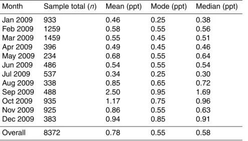
The CH3I mixing ratios at Tawau (∼8400 in total) vary from below 0.1 up to 11 ppt,

with the large majority of points towards the lower end of the range. July sees the low-est monthly mean of 0.34 ppt and the highlow-est monthly mean of 2.50 ppt is in

Septem-15

ber. The highest values and the greatest variability are observed in September and

October. Back-trajectories indicate that air containing high amounts of CH₃I had

pre-viously passed over large biomass burning events in southern Borneo (as observed

by MODIS). Emissions of CH3I in biomass burning have been reported previously

(An-dreae et al., 1996; Mead et al., 2008c). However while biomass burning emissions may

20

be significant locally at some times of year, it is not the case globally (Bell et al., 2002;

Butler et al., 2007). Interestingly some of the lowest observed values (<0.1 ppt) of CH3I

occur when the air has previously been in the terrestrial boundary layer, indicating that

the tropical rainforests were not normally a source of CH3I. The seasonal cycle in the

baseline (i.e. if the high values seen in the late summer/early autumn are excluded) at

25

(22)

ACPD

14, 1919–1969, 2014

Title Page

Tables Figures

◭ ◮

Back Close

Full Screen / Esc

Discussion

P

a

per

|

D

iscussion

P

a

per

|

Discussion

P

a

per

|

Discuss

ion

P

a

per

|

5.5 Total bromine

Here we present and discuss our observations of bromine defined as [CHBr3]+

[CH2Br∗2] as an approximate measure of total organic bromine from the two sites. For

a two week period of the OP3 campaign (5–12 July 2008) we ran our Bukit Atur

instru-ment alongside a GC-MS system from UEA which measured CHBr3, CH2Br2, CHBr2Cl,

5

CHBrCl2 and CH2BrCl (the five main naturally occurring bromine source gases). The

GC-MS observations showed that CHBr₃and CH₂Br₂accounted for 93.5 % of the total

Br coming from these five bromine source gases (Pyle et al., 2011a). Total bromine as

[CHBr3]+[CH2Br∗2] from our measurements at Tawau over the period November 2008

to January 2010 is shown as a time series in Fig. 8a. The black line through the data

10

is the running average total bromine (40 point, 50 pass) to highlight average

variabil-ity. Bromine from these two compounds (accounting for>90 % of the total organic Br)

averages 9.7 ppt over the period of observations and ranges from 3.7 ppt (June 2009) to 189.5 ppt (December 2008). The probability distribution function for total observed

bromine as [CHBr3]+[CH2Br∗2] at Bukit Atur is compared with that for Tawau in Fig. 8b.

15

The distributions are similar (median values of 6.79 and 7.97 ppt at Bukit Atur and Tawau respectively) and Bukit Atur has a narrower inter-quartile range than Tawau (2.06 ppt compared to 2.80 ppt). The extended tail of very high total bromine values

(>20 ppt) is evident at Tawau and completely absent from the Bukit Atur observations.

The fact that the observations of bromine from [CHBr3]+[CH2Br∗2] are so similar at

20

both sites (with the exception of the very high coastal values) shows that an inland site

can be used effectively to make regional observations suited to model comparison. In

fact as the model we used here was unable to capture the very high temporal (and we assume spatial) variability seen at the coast we would suggest that, for evaluating models, an inland site is preferable to a coastal site. We also calculate total modelled

25

bromine coming from [CHBr₃]₊[CH₂Br₂] in p-TOMCAT at Tawau and find for the period

(23)

ACPD

14, 1919–1969, 2014

Title Page

Tables Figures

◭ ◮

Back Close

Full Screen / Esc

Discussion

P

a

per

|

D

iscussion

P

a

per

|

Discussion

P

a

per

|

Discuss

ion

P

a

per

|

Our data provide a longer-term context for other reports from short campaign-type observations. There are month-to-month variations in total Br in our data that would be missed by shorter deployments. Overall, our mean value of 9.7 ppt from

[CHBr₃]+[CH₂Br∗₂] seems quite consistent with other work in the region. There have

been somewhat conflicting reports of the fraction of Br in CHBr3and CH2Br2compared

5

to the minor VSLS. Montzka and Reimann (2011) suggest a boundary layer median

value of 8.4 ppt Br from VSLS, with 83 % from CHBr₃(1.6 ppt×3) and CH2Br2(1.1 ppt

×2). Based on data obtained in July 2008 from the OP3 campaign, Pyle et al. (2011a)

report 7 ppt (5–10 ppt) Br from VSLS, with over 90 % of this present as CHBr3, CH2Br2

or CHBrCl₂. Nadzir et al. (2013) report a mean of 8.9 ppt Br from all VSLS (range 5.2 to

10

21.4 ppt in individual samples), with∼90 % from CHBr3and CH2Br2during the Prime

Expedition Scientific Cruise during June and July 2009.

6 Summary

Until recently, few measurements of short-lived halogenated compounds had been made in southeast Asia. These compounds have significant atmospheric importance,

15

and previous studies have speculated that southeast Asia represents an unusually

strong source of the naturally occurring species (e.g. CHBr3). Here we present more

than one year of observations (November 2008 to January 2010) of key short-lived compounds from a coastal (Tawau) and an inland (Bukit Atur) site in this region, which together provide valuable data to the atmospheric science community. The data have

20

been placed on the HalOcAt database for community access (https://halocat.geomar. de/). The data allow seasonal cycles, emissions and the role of local and long range transport to be studied.

By combining the observations with air mass history information generated by NAME

we explain the strong seasonal cycle seen in the anthropogenic tracer (C2Cl4). From

25

(24)

ACPD

14, 1919–1969, 2014

Title Page

Tables Figures

◭ ◮

Back Close

Full Screen / Esc

Discussion

P

a

per

|

D

iscussion

P

a

per

|

Discussion

P

a

per

|

Discuss

ion

P

a

per

|

masses originate from regions to the south (typical mixing ratio 0.5 ppt). The overall

median values for C2Cl4are 1.33 ppt and 0.99 ppt at Bukit Atur and Tawau respectively.

The naturally occurring brominated tracers CHBr3and CH2Br∗2 do not show

unam-biguous seasonal variation, though there is a slight hint of a seasonal cycle in CH₂Br∗₂.

Both compounds nevertheless show strong variability over shorter timescales. At the

5

coast, the CHBr3 observations occasionally peak at over 100 ppt compared with the

overall median level of 1.7 ppt. At Bukit Atur, the overall inland median level for CHBr₃

is 1.6 ppt and the occasional peaks are much lower than at the coast with maximum

observations of just over 5 ppt. Coastal CH2Br∗2mixing ratios occasionally rise to over 7

times the median level of 1.4 ppt, whereas inland the maximum level observed is a little

10

over 2 ppt. The strong coastal variability of both these compounds is likely related to the strongly heterogeneous nature of their marine sources, which are believed to be a combination of coastal macroalgae and both coastal and oceanic microalgae. Ac-cordingly, the measurements from coastal Tawau are more variable than at Bukit Atur, being made closer to these sources.

15

The observations of CHBr3and CH2Br∗2also provide a valuable longer term estimate

of the contribution to total Br in the boundary layer from the main naturally occurring short-lived brominated compounds. At the coast we observe an overall median value

of Br from CHBr3and CH2Br∗2of 8.0 ppt and inland the overall median value is 6.8 ppt.

These values are reasonably consistent with other recent estimates of this quantity

20

based on much shorter measurement periods. Our data provide evidence that south-east Asia may not in fact be a region of enhanced brominated VSLS emissions into the boundary layer in relation to other tropical locations where similar measurements have been made.

Our coastal observations of CH3I show high variability as expected for a short lived

25

(25)

ACPD

14, 1919–1969, 2014

Title Page

Tables Figures

◭ ◮

Back Close

Full Screen / Esc

Discussion

P

a

per

|

D

iscussion

P

a

per

|

Discussion

P

a

per

|

Discuss

ion

P

a

per

|

times of the year, air that passed over land showed some of the lowest values observed,

indicating that the tropical rain forests in Borneo are not a source of CH3I.

To date, modelling work has focussed on understanding our CHBr3data. The CHBr3

observations presented here were recently used by Ashfold et al. (2013), along with

NAME trajectories and an inversion method, to estimate regional scale CHBr3

emis-5

sions. When extrapolated across the global tropics, the magnitude of their estimated emissions was somewhat lower than most other recent estimates, which have tended to assume strong emissions in southeast Asia. This is consistent with the finding here,

that observed CHBr3 mixing ratios in Borneo (and indeed CH2Br∗2 mixing ratios and

total Br estimates) are in fact similar to those measured in other parts of the world.

10

Our measurements also provide a means of testing the ability of global models like p-TOMCAT to reproduce boundary layer time series of short-lived compounds in tropical regions. Although p-TOMCAT was unable to reproduce the same magnitude of

variabil-ity seen in the Borneo CHBr₃observations, it was able to capture background

concen-trations using the bromoform emission distribution described in Pyle et al. (2011). This

15

emission distribution is an updated version of the distribution described in Warwick et al. (2006), containing substantial reductions in southeast Asian emissions relative to the original scenario.

We continue to make halocarbon measurements in Sabah and have upgraded to the newer version of µDirac with a 20 m long column and better resolution of species

20

including CH2Br2. In addition, we have recently begun measuring the same group of

compounds using upgraded versions of the instruments used here at three other sites in the southeast Asia region: at Bachok on the Malaysian peninsula, Kelantan state; at Gunn Point near Darwin, Australia; a coastal site near Taipei, Taiwan. These sites significantly extend the geographic coverage of our measurements.

25

Acknowledgements. This work was supported by a NERC consortium grant to the OP3

(26)

stu-ACPD

14, 1919–1969, 2014

Title Page

Tables Figures

◭ ◮

Back Close

Full Screen / Esc

Discussion

P

a

per

|

D

iscussion

P

a

per

|

Discussion

P

a

per

|

Discuss

ion

P

a

per

|

dentships. Andrew Robinson acknowledges NERC for their support through small grant project NE/D008085/1. Neil Harris is supported by a NERC Advanced Research Fellowship. We thank The Sabah Foundation, Danum Valley Field Centre and the Royal Society (Glen Reynolds) for field site support. The research leading to these results has received funding from the European

Union’s Seventh Framework Programme FP7/2007–2013 under grant agreement n◦ _{226224 –}

5

SHIVA. We thank David Oram and Stephen Humphrey at UEA for their assistance in checking the calibration of our Aculife cylinder in May 2009.

This is paper numberZ of the Royal Society’s South East Asian Rainforest Research

Pro-gramme.

References

10

Amachi, S., Kamagata, Y., Kanagawa, T., and Muramatsu, Y.: Bacteria mediate methylation of iodine in marine and terrestrial environments, Appl. Environ. Microb., 67, 2718–2722, 2001. Andreae, M. O., Atlas, E., Harris, G. W., Helas, G., de Kock, A., Koppmann, R., Maenhaut, W.,

Manø, S. M., Pollock, W. H., Rudolph, J., Scharffe, D., Schebeske, G., and Welling, M.: Methyl

halide emissions from savanna fires in southern Africa, J. Geophys. Res., 101, 23603–

15

23613, 1996.

Aschmann, J., Sinnhuber, B.-M., Atlas, E. L., and Schauffler, S. M.: Modeling the transport

of very short-lived substances into the tropical upper troposphere and lower stratosphere, Atmos. Chem. Phys., 9, 9237–9247, doi:10.5194/acp-9-9237-2009, 2009.

Ashfold, M. J., Harris, N. R. P., Manning, A. J., Robinson, A. D., Warwick, N. J., and Pyle, J. A.:

20

Estimates of tropical bromoform emissions using an inversion method, Atmos. Chem. Phys. Discuss., 13, 20463–20502, doi:10.5194/acpd-13-20463-2013, 2013.

Bell, N., Hsu, L., Jacob, D. J., Schultz, M. G., Blake, D. R., Butler, J. H., King, D. B., Lobert, J. M., and Maier-Reimer, E.: Methyl iodide: Atmospheric budget and use as a tracer of marine con-vection in global models, J. Geophys. Res., 107, 4340, doi:10.1029/2001JD001151, 2002.

25

(27)

ACPD

14, 1919–1969, 2014

Title Page

Tables Figures

◭ ◮

Back Close

Full Screen / Esc

Discussion

P

a

per

|

D

iscussion

P

a

per

|

Discussion

P

a

per

|

Discuss

ion

P

a

per

|

Brownell, D. K., Moore, R. M., and Cullen, J. J.: Production of methyl halides by Prochlorococ-cus and SynechococProchlorococ-cus, Global Biogeochem. Cy., 24, 1–7, doi:10.1029/2009GB003671, 2010.

Butler, J. H., King, D. B., Lobert, J. M., Montzka, S. A., Yvon-Lewis, S. A., Hall, B. D., Warwick, N. J., Mondeel, D. J., Aydin, M., and Elkins, J. W.: Oceanic

distribu-5

tions and emissions of short-lived halocarbons, Global Biogeochem. Cy., 21, GB1023, doi:10.1029/2006GB002732, 2007.

Carpenter, L. J. and Liss, P. S.: On temperate sources of bromoform and other reactive bromine gases, J. Geophys. Res., 105, 20539–20547, doi:10.1029/2000JD900242, 2000.

Carpenter, L. J., Jones, C. E., Dunk, R. M., Hornsby, K. E., and Woeltjen, J.: Air-sea fluxes

10

of biogenic bromine from the tropical and North Atlantic Ocean, Atmos. Chem. Phys., 9, 1805–1816, doi:10.5194/acp-9-1805-2009, 2009.

Cook, P. A., Savage, N. H., Turquety, S., Carver, G. D., O’Connor, F. M., Heckel, A., Stew-art, D., Whalley, L. K., Parker, A. E., Schlager, H., Singh, H. B., Avery, M. A., Sachse, G. W., Brune, W., Richter, A., Burrows, J. P., Purvis, R., Lewis, A. C., Reeves, C. E., Monks, P. S.,

15

Levine, J. G., and Pyle, J. A.: Forest fire plumes over the North Atlantic: p-TOMCAT model simulations with aircraft and satellite measurements from the ITOP/ICARTT campaign, J. Geophys. Res., 112, D10S43, doi:10.1029/2006JD007563, 2007.

Davies, T., Cullen, M. J. P., Malcolm, A. J., Mawson, M. H., Staniforth, A., White, A. A., and

Wood, N.: A new dynamical core for the Met Office’s global and regional modelling of the

20

atmosphere, Q. J. Roy. Meteor. Soc., 131, 1759–1782, 2005.

Derwent, R. G., Simmonds, P. G., Greally, B. R., O’Doherty, S., McCulloch, A., Manning, A. J., Reimann, S., Folini, D., and Vollmer, M. K.: The phase-in and phase-out of European emis-sions of HCFC-141b and HCFC-142b under the Montreal Protocol: evidence from observa-tions at Mace Head, Ireland and Jungfraujoch, Switzerland from 1994–2004, Atmos.

Envi-25

ron., 41, 757–767, 2007.

Dorf, M., Butler, J. H., Butz, A., Camy-Peyret, C., Chipperfield, M. P., Kritten, L., Montzka, S. A., Simmes, B., Weidner, F., and Pfeilsticker, K.: Long-term observations of stratospheric bromine reveal slow down in growth, Geophys. Res. Lett., 33, L24803, doi:10.1029/2006GL027714, 2006.

30