Essays on illiquidity premium

(1)

FUNDAÇÃO GETULIO VARGAS ESCOLA DE ECONOMIA DE SÃO PAULO

RICARDO BUSCARIOLLI PEREIRA

ESSAYS ON ILLIQUIDITY PREMIUM

(2)

Tese apresentada à Escola de Economia de São Paulo da Fundação Getulio Vargas como requisito para a obtenção do título de doutor em economia.

Área do conhecimento: Economia Financeira

Orientador: João Filipe Bernardes Volkmann de Mendonça Mergulhão

(3)

Pereira, Ricardo Buscariolli.

Essays on illiquidity premium /Ricardo Buscariolli Pereira - 2014.

170 f.

Orientador: João Filipe Bernardes Volkmann de Mendonça Mergulhão

Tese (doutorado) - Escola de Economia de São Paulo.

1. Liquidez (Economia). 2. Finanças. 3. Mercado de capitais. 4. Investimentos. I. Mergulhão, João Filipe Bernardes Volkmann de Mendonça. II. Tese (doutorado) - Escola de Economia de São Paulo. III. Título.

(4)

Tese apresentada à Escola de Economia de São Paulo da Fundação Getulio Vargas como requisito para a obtenção do título de doutor em economia.

Área do conhecimento: Economia Financeira Data da aprovação

23/05/2014

Banca examinadora:

Prof. Dr. João Filipe Bernardes Volkmann de Mendonça Mergulhão (Orientador) – Escola de Economia de São Paulo – Fundação Getulio Vargas (EESP-FGV)

Prof. Dr. Marcelo Fernandes - Escola de Economia de São Paulo – Fundação Getulio Vargas (EESP-FGV)

Prof Dr. Pedro Valls Pereira - Escola de Economia de São Paulo – Fundação Getulio Vargas (EESP-FGV)

Prof. Dr. Fernando Daniel Chague – Faculdade de Economia, Administração e Contabilidade – Universidade de São Paulo (FEA-USP)

(5)

(6)

AGRADECIMENTOS

It would have been impossible for me to finish anything without the help of many. First, I would like to thank my advisor Prof. João Mergulhão for all his help and guidance. I hope I am the first tutee of many to come.

I am very grateful to Prof. Marcelo Fernandes and Prof. Pedro Valls Pereira for all the attention, help and suggestions. I would also like to thank the members of the committee for all the insights and contributions.

My colleagues and friends from the EESP-FGV helped me countless times. I am deeply thankful to Alessandro Casalecchi, André Barbosa Oliveira, Caio Mussolini, Diogo de Prince Mendonça, Felippe Serigati, Luis Fernando Azevedo, Marcio Pereira Swistalski, Marília Gabriela Elias da Silva, Ricardo Politi, Rodrigo Barbosa, Thiago De Lucena and Wagner Monteiro.

I had the chance of interacting with many professors who helped me in many aspects to achieve this degree. I would like to thank professors Braz Camargo, Emerson Marçal, Enlinson Mattos, Klenio Barbosa, Olivier Scaillet, Ramon Garcia-Fernandez and Rodrigo De Losso.

I would also like to express my gratitude to my family who always supported and stood by my side. In special, I am very grateful to my mother who made many sacrifices for me to pursue my education. In this four-year period many friends were of great support and would not allow me to give up. Some of them are probably not even aware of how helpful they were in motivating me to keep going. I would like to thank André Garcia, Andrea Carucci, Fabio Dantas, Gabriela Buraschi, Humberto Cacioli, Jander Minesso, Jorge Marega, Luiz Henrique Oriani, Rafael Madrona, Raffaello Starace, Rebecca Alvarez Inhesta, Renato Madrona, Roberto Aragão, Sofia Calcagno, Thiago Rodrigues, Thiago Zamorano and Vitor Puppin.

I am very grateful to Johanna Löwgren who put up with me and was a never-ending source of motivation in the toughest moments of the whole workflow.

(7)

ABSTRACT

This dissertation is composed of three related essays on the relationship between illiquidity and returns. Chapter 1 describes the time-series properties of the relationship between market illiquidity and market return using both yearly and monthly datasets. We find that stationarized versions of the illiquidity measure have a positive, significant, and puzzling high premium. In Chapter 2, we estimate the response of illiquidity to a shock to returns, assuming that causality runs from returns to illiquidity and find that an increase in firms' returns lowers illiquidity. In Chapter 3 we take both effects into account and account for the endogeneity of returns and illiquidity to estimate the liquidity premium. We find evidence that the illiquidity premium is a smaller than the previous evidence suggests. Finally, Chapter 4 shows topics for future research where we describe a return decomposition with illiquidity costs.

JEL classification: G12

(8)

RESUMO

Esta tese é composta por três ensaios sobre a relação entre iliquidez e retornos. O Capítulo 1 descreve as propriedades de séries de tempo da relação entre iliquidez e retorno de mercado utilizando dados anuais e mensais. Os resultados mostram que a versão estacionarizada da medida de iliquidez tem um efeito postivo, significante e alto sobre o retorno de mercado. No capítulo 2, estimo a resposta da iliquidez a um choque no retorno de mercado, assumindo que a direção da causalidade se dá do retorno para a iliquidez e mercado. Os resultados indicam que um aumento no retorno reduz a iliquidez de mercado. No capítulo 3 os dois efeitos são considerados mutuamente levando em conta a endogeneidade entre retornos e iliquidez. Os resultados mostram que o prêmio de liquidez é menor do que a evidência prévia sugere. Finalmente, o capítulo 4 exibe tópicos de pesquisa futura e descreve uma decomposição de retornos com custos de iliquidez.

(9)

List of Tables

1.1 Descriptive statistics of yearly data 26

1.2 Tests for unit root - Yearly 29

1.3 Descriptive statistics - Monthly 32

1.4 Tests for unit root - Monthly 35

1.5 Price of the Yearly Amihud (2002) Measure 45

1.6 Measuring Unexpected Amihud (2002) Measure - Yearly 47

1.7 Price of Yearly Amihud’s (2002) Measure with the Unexpected Illiquidity given by an AR(1) 49

1.8 Price of Yearly Amihud’s (2002) measure with the unexpected illiquidity given by an MA(2) 50

1.9 Pricing of the Yearly market Turnover-Version Amihud (2002) measure 52

1.10 Price of Yearly turnover-version Amihud (2002) measure with the unexpected illiquidity given by an AR(1) 54

1.11 Price of the Monthly Amihud (2002) Measure 56

1.12 Price of the Monthly Amihud (2002) Measure AR(1) 59

1.13 Measuring unexpected Amihud’s (2002) measure - Monthly 60

1.14 Price of Monthly Amihud’s (2002) measure with the unexpected illiquidity given by an AR(1) 62

1.15 Price of monthly Amihud’s (2002) measure with the unexpected illiquidity given by an AR(2) 63

1.16 Akaike (AIC) and Bayesian (BIC) Information Criteria for monthly data 65

1.17 Price of the Monthly Amihud (2002) Measure - Illiquidity lagged twice 67

1.18 Pricing of the Monthly market Turnover-version Amihud (2002) measure 68

1.19 Autoregressive Distributed Lag (ARDL) model with market Turnover measure and size 70

1.20 Quasi-Local Level (QLL) - Yearly 72

1.21 Quasi-Local Level (QLL) - Monthly 72

2.1 Descriptive statistics 80

2.2 Illiquidity response to a change in …rms’s returns - Yearly Cross-Section 82

2.3 Illiquidity response to a change in …rms’s returns - Monthly Cross-Section 83

2.4 Response of market illiquidity to changes in market return - Yearly 87

2.5 Response of market illiquidity to changes in market return - AR(1) - Yearly 88

2.6 Response of market illiquidity to changes in market return - Monthly 90

(10)

3.1 Reduced form VAR - Monthly data 114

3.2 Structural VAR - Monthly - Coe¢cients of the matrix of short-run restriction 116

3.3 Structural VAR - Monthly - Structural coe¢cients estimated with short-run restriction and …rst-di¤erenced

log-transformed illiquidity 117

3.4 Structural VAR - Monthly - Structural coe¢cients estimated with short-run restriction and …rst-di¤erenced

HP-…ltered illiquidity 118

3.5 Structural VAR - Monthly - Structural coe¢cients estimated with long-run restriction and …rst-di¤erenced

log-transformed illiquidity 119

3.6 Structural VAR - Monthly - Structural coe¢cients estimated with long-run restriction and HP-…ltered

(11)

Introduction

This dissertation is composed of three related essays on the relationship between

illiq-uidity and returns. Chapter 1 describes the time-series properties of the relationship

between market illiquidity and market return using both yearly and monthly datasets.

We update the dataset of Amihud (2002) and …nd that the illiquidity measure he suggests

is non-stationary and, as such, yields a non-signi…cant illiquidity premium. We …nd, on

the other hand, that if we work with stationarized versions of the illiquidity measure we

…nd a premium that is positive and signi…cant, both statistically and economically.

Nev-ertheless, the estimated illiquidity premium is still puzzling high, as previous evidence

suggests.

In Chapter 2, we estimate the response of illiquidity to a shock to returns, assuming

that causality runs from returns to illiquidity. We analyze and con…rm the cross-section

evidence of Hameed, Kang and Viswanathan (2010). However, we use the daily Amihud

(2002) measure of illiquidity instead of the intraday proxy they construct and …nd that

an increase in …rms’ returns lowers illiquidity. We also analyze time-series properties and

…nd that a higher than average market return lowers market illiquidity. This implies that

the direction of the relationship between return and illiquidity is di¤erent from the one

in Chapter 1.

In Chapter 3, we relax the causality assumptions of the previous Chapters and take the

endogeneity of returns and illiquidity into account to estimate the liquidity premium. We

use an structural vector autoregression framework to estimate the illiquidity premium,

ac-counting for the dynamic relation between market return and illiquidity. We …nd evidence

that the illiquidity premium is a smaller than the previous evidence suggests, showing that

(14)

that, using monthly data, the models yield non-signi…cant coe¢cients at any level. That

may suggest that at higher frequencies prices anticipate the information about illiquidity.

Finally, Chapter 4 shows topics for future research where we describe a return

(15)

(16)

CHAPTER 1

(17)

Abstract

In this Chapter we study the time series properties of Amihud (2002) illiquidity

mea-sure. We …nd that this measure is non-stationary, which has consequences to the

esti-mation of the illiquidity premium over time. We use di¤erent stationarized versions of

illiquidity and also use an Autoregressive Distributed Lag (ARDL) model after

decompos-ing the original Amihud’s (2002) measure into two non-stationary variables: the turnover

version of the illiquidity measure and size. To the best of our knowledge such an analysis

is novel and the conclusions of it are important for estimating the illiquidity premium in

(18)

1.1. Introduction

In this Chapter we study the time series properties of the illiquidity premium. We

start by revisiting the time series evidence on the relation between illiquidity and returns

using Amihud (2002) illiquidity measure. Our …ndings support the notion that illiquidity

is priced for both yearly and monthly data. However, this result does not hold if we use

the non-stationarized original measure of Amihud (2002).

Both yearly and monthly data are analyzed to check any potential di¤erence in the two

frequencies. Results suggest that yearly and monthly illiquidity are priced and that this

price is puzzling high, in line with the cross-sectional evidence. These results, however,

depend on the strategy we use to convert the illiquidity measure into a stationary variable.

The non-stationarity of Amihud (2002) measure seem to be playing a major role in

this analysis. This measure has a negative trend over the years and this was not taken into

account in Amihud (2002). His sample ends in 1995, which could have perhaps blurred

some of the conclusions about non-stationarity. However, by updating the data sample,

it is clear that stationarity has to be addressed. In fact, as market return is a stationary

variable, using a non-stationary regressor leads to the conclusion that its coe¢cient of

illiquidity is non-signi…cant at any conventional level.

We …rst tackle this issue by revisiting Amihud’s (2002) approach using updated data,

from 1962 to 2011. We make the illiquidity measure stationary by both taking the …rst

di¤erence and …ltering it, following the methodology proposed by Hodrick and Prescott

(1981). We also estimate coe¢cients using the same approach of Amihud (2002), i.e., using

non-stationary illiquidity as a regressor. We do that to be consistent with his previous

work and also to discuss the results and access the gains of adjusting the variables.

Amihud’s (2002) measure uses the dollar volume of trading as the proxy of trading

activity. Brennan, Huh and Subrahmanyam (2013) (henceforth, BHS) suggest that the

estimation of the illiquidity premium should use a measure of illiquidity that relies on

turnover as the proxy of trading activity to account separately for …rm size e¤ects.

(19)

(2002) scales illiquidity with …rm size: smaller stocks which have smaller dollar volume

for the same turnover (fraction of outstanding shares that are traded) are automatically

more illiquid (Cochrane, 2005; Florakis, Gregoriou, and Kostakis, 2011).

Following BHS approach, we decompose the illiquidity measure into turnover and size

and re-estimate the illiquidity premium. The results for yearly data show an illiquidity

premium that is not as high as the one we …nd for the original measure. Monthly data

yield negative coe¢cients and their values do not seem to be more "reasonable", as BHS

argue.

The BHS illiquidity decomposition allows a di¤erent approach for making the

illiquid-ity measure stationary. If the turnover and size components cointegrate, we can re-specify

the model to get the estimated illiquidity premium. Although we do not …nd a

cointe-gration relationship at the yearly level, monthly data evidence suggest that these two

components have a long term relationship. Nevertheless, using an Autoregressive

Distrib-uted Lag (ARDL) model, the illiquidity premium for the turnover illiquidity version is

non-statistical signi…cant at any conventional level.

In Amihud’s (2002) time series analysis, the author also studies the e¤ect of

"un-expected illiquidity" over returns. He suggests that, although "un-expected illiquidity has

a positive impact over the following period’s market returns, an increase in unexpected

illiquidity decreases contemporaneous market return. This is a consequence of the

adjust-ment mechanism: when market illiquidity goes up, the price level in the contemporaneous

period goes down, thus increasing next period’s (and decreasing the current period’s)

re-turn. If the model does not explicitly consider the e¤ect of that unexpected illiquidity,

the coe¢cients may be biased. We also address this issue and, following Amihud (2002),

we assume that agents expect illiquidity to be an AR(1) process. The di¤erences between

"realized" and expected illiquidity are due to the "unexpected" component.

We add this feature to the speci…cations that use the turnover versions of illiquidity

as well. Results suggest that unexpected illiquidity indeed has a negative impact over

(20)

of the coe¢cients of the illiquidity variables remain almost unchanged when adding the

unexpected component. We test additional models for predicting the expected illiquidity,

for robustness, and …nd no major di¤erence in results.

The …nal exercise of this Chapter is to check the stability of the estimated models over

time. We do so by using the Elliott and Muller’s (2006) Quasi-Local Level (QLL) test.

Amihud (2002) also addresses this question and …nds that his speci…cation is stable. We

…nd evidence that the parameters we estimate using Amihud’s (2002) speci…cation are not

stable, however, the models that use the stationarized variables are. In other words, the

model using Amihud’s (2002) measure is not stable but when we transform the variables

into some stationary form it is.

The contributions of the Chapter can be summarized as:

1) Using a recent sample, we comprehensively analyze the time series properties of

Amihud’s (2002) illiquidity measure, and show that it is non-stationary, an issue that

was ignored so far. We show that the illiquidity premium is statistical signi…cant on the

extended sample only if stationarity is addressed.

2) We analyze the monthly premium of the market Amihud (2002) measure. As far

as we know this is the …rst time the monthly data is considered in a time series study,

whereas BHS only study the cross-sectional properties;

3) We use the turnover decomposition of BHS in the time series analysis and measure

the premium associated with this variable.

Chapter 1 is organized as follows: section 1.2 presents Amihud’s (2002) measure of

illiquidity and how it is decomposed into the BHS turnover version; section 1.3 describes

the estimation procedures; section 1.4 describes the data we use throughout this

disser-tation; section 1.5 describes the results for both yearly and monthly data and deals with

(21)

1.2. Measures of Illiquidity

What drives the relationship between liquidity and returns is that market makers

cannot distinguish between order ‡ows generated by informed traders and by noise traders.

Therefore, they set prices that are an increasing function of the imbalance in the order

‡ow (which may indicate informed trading) (Amihud, 2002; Amihud and Mendelson,

1980; Glosten and Milgrom, 1985). This creates a positive relationship between the order

‡ow or transaction volume and price change, commonly called "price impact".

The evidence on the relationship between liquidity and return is quite vast. Many

papers argue that liquidity has an impact on the expected return and price of an asset,

what Amihud and Mendelson (1991) call “liquidity e¤ect”. Under this point of view,

illiquid assets and assets with high transaction costs trade at low prices relative to their

intrinsic values, in other words, liquidity is priced (Amihud and Medenlson, 1986; Brennan

and Subrahmanyam, 1996; Datar, Naik and Radcli¤e, 1998; Chordia, Subrahmanyam and

Anshuman, 2001).

The liquidity e¤ect is, in broad terms, related to the e¤ect of risk on the returns

of assets. The idea is that agents prefer liquid investments that can be traded quickly

and at low costs anytime they are in need. Therefore, less liquid investments must o¤er

higher expect returns in order to attract investors in the same way a risk-averse investor

would require a higher expected return as a compensation for greater risk (Amihud and

Medelson, 1991).

This relationship has been extended in a variety of ways such as in Vayanos (1998),

Lo, Mamaysky and Wang (2004); Eisfeldt (2004); Holmstrom and Tirole (2002); Huang

(2003), and O’Hara (2003). Acharya and Pedersen (2005), for example, develop a model

considering factors related to commonality and risk premia associated with changes in

liquidity, …nding di¤erent risk premia associated with changes in liquidity which turned

out to be highly signi…cant in empirical work.

Empirical evidence support this notion that liquidity explains part of the expected

(22)

two variables are positively related. This suggests that expected stock excess return partly

represents an illiquidity premium. Jones (2002) …nds that bid-ask spreads and turnover

predict U.S. stock returns one period ahead. Another feature found in empirical analysis

is that, if liquidity varies systematically, securities whose returns are positively correlated

with market liquidity should have higher expected returns (Pastor and Stambaugh (2002);

Sadka (2002); Chordia, Roll, and Subrahmanyam (2000); Huberman and Halka (1993)).

There are many liquidity measures and Goyenko, Holden and Trzcinka (2008) show

that most of them do a good job on measuring liquidity. They horserace some of these

measures, such as Amihud (2002) and Pastor and Stambaugh (2002), considering both

price impact and e¤ective spread criteria. They show that among the realized spread

measures, Amihud’s (2002) is the best overall. They also show that Pastor-Stambaugh

Gamma, is dominated by much simpler measures.

Amihud (2002) measure can also be used to uncover the relative impact of turnover

and illiquidity over returns. This is the approach taken by BHS, who show that the

return premium is "better" captured when turnover (instead of dollar volume) is used to

construct the Amihud measure, and …rm size e¤ects are accounted for separately. What

quali…es it as "better" in BHS is, however, related to what they call a more "reasonable"

measure, as the premium estimated using it is not as puzzling high as the one related to

Amihud (2002). In the next subsection we show how we calculate the yearly and monthly

Amihud (2002) original measure of illiquidity, as well as its turnover version.

1.2.1. Amihud (2002) measure and the turnover version

Amihud (2002) develops an illiquidity measure based on the price impact caused by

trad-ing volume that became very popular. We follow the notation of BHS: for security i in each trading day we calculate

(1.1) A0i;d =

jri;dj

(23)

where ri;d is the daily stock return of security i on day d, and; DV OLi;d is daily dollar volume of securityion dayd:This measure represents the daily price response associated with one dollar of trading volume. Amihud (2002) argues that this illiquidity measure is

strongly related to the liquidity ratio known as the Amivest measure, the ratio of the sum

of the daily volume to the sum of the absolute return (Khan and Baker, 1993). It is also

positively related to variables that measure illiquidity from microstructure data such as

Kyle’s (1985) price impact.

The inclusion of this measure in the regression hides, however, the relative importance

for asset pricing of turnover and …rm size. In order to get these separate e¤ects we

decompose the original Amihud (2002) measure (A0) into its turnover version (A) and a size-related element (S) as in BHS. First, note that the daily dollar volume of security i on dayd (DV OLi;d) is de…ned as the multiplication of the total number of shares by the price on dayd as

(1.2) DV OLi;d =V oli;d pi;d

whereV oli;d is the volume traded of security ion day d, and;pi;d is the price of securityi on dayd. Note, also, that the turnover of securityi on dayd; Ti;d;is de…ned as the daily share volume divided by the total number of shares outstanding

(1.3) Ti;d =:

V oli;d

#sharesi;d

where #sharesi;d is the total number of shares outstanding of security i on day d. We can, therefore, write Amihud’s (2002) measure for a given securityi in a given day d as

(1.4) A0_i;d = jri;dj

DV OLi;d

= jri;dj

Ti;d

(24)

whereTi;d is the turnover of security ion day d: Note that, by de…nition, the ratio

(1.5) Ti;d

DV OLi;d

can be written as

Ti;d DV OLi;d

=

V oli;d #sharesi;d

V oli;d pi;d

whereV oli;d is the share volume of securityion day d;#sharesi;d is the total number of shares outstanding of securityi on dayd, and; pi;d is the price of securityi on dayd. By simple algebra we have

Ti;d DV OLi;d

= V oli;d #sharesi;d

1

V oli;d pi;d

= 1

#sharesi;d pi;d

= 1

Si;d

where S is …rm i’s Size, i.e., the market capitalization of …rm i. Hence, we can re-write A0

i;d as

(1.6) A0_i;d = jri;dj

Ti;d

1

Si;d

=Ai;t

1

Si;d

By taking natural logarithms on both sides of Equation (1.6) we get the relation

betweenA0

i;d,Ai;d and …rm size,Si;d

(25)

Once we calculate the Amihud (2002) measure for each day we construct the monthly

measure for security i by averaging the ratio jri;dj

DV OLi;d over all the days of the month for

each month. We repeat the same process for the yearly measure, averaging it over all the

days in each year. Formally, the monthly measure is given by

(1.8) A0i;m=

1

Di;m D_Xi;m

d=1

jri;dj

DV OLi;d

where Di;m is the number of trading days of security i in month m; jri;dj is the absolute return of securityi on dayd ;and; DV OLi;d is the trading volume (in units of currency) on dayd.

The yearly measure for a given …rm iover yeary, de…ned as the yearly average of the daily measure, is given by1

(1.9) A0_i;y = 1

Di;y Di;y

X

d=1

jri;dj

DV OLi;d

where Dy is the number of trading days in year y; jri;dj is the absolute return on day d for securityi; DV OLi;d is the trading volume (in units of currency) on day d.

BHS do the same for Ai;m and Si;m, i.e., they de…ne the monthly turnover version of Amihud’s (2002) measure, Ai;m, as

1_{Amihud (2002) has another step after calculating}_A0

i;y. He also calculates the average market illiquidity across securities in each year

A0_EW;y= 1

Ny Nt

X

i=1 A0_i;y

In which Nt is the number of securities in yeary. This average illiquidity varies considerably over the years, for that reasonA0

i;y is replaced by its mean-adjusted value

A0_i;y;M A= A

0 i;y

A0 EW;y

(26)

(1.10) Ai;m = 1 Di;m Di;m X d=1

jri;dj

Ti;d

and size,Si;m, as the average of daily market values within a month

(1.11) Si;m =

1

Di;m D_Xi;m

d=1

(#sharesi;d pi;d)

Note that the exact equivalence between the A0_i;m and Ai;m does not hold taking this approach. That happens because2

(1.12) A0i;m=

1

Di;m D_Xi;m

d=1

jri;dj

DV OLi;d

= 1

Di;m D_Xi;m

d=1 Ai;t 1 Si;d 6 = 1 Di;m

PDi;m

j=1 Ai;t

1

Di;m

PDi;m

j=1 Si;d

Thus, the monthly and yearly turnover versions of Amihud (2002) measure, as

cal-culated by BHS, are not exactly equivalent to the original Amihud’s (2002) measure.

However, for a matter of consistency, we let those variables as calculated by BHS (2013)

in our paper. An alternative would have been to take the logs and then take the average,

which is just the geometric mean. However, the logarithm function is not de…ned for zero

returns, which is commonly observed in daily data, and for this reason the measure would

su¤er some sort of bias. Therefore the implicit assumption in BHS is that

2_{It is actually possible to show how di¤erent}_EhAi;m Si;m

i

is from E_E(₍Ai;m_Si;m₎) . Taking the bivariate …rst order Taylor expansion ofA0

i;m= Ai;m

Si;m about a given point yields

E Ai;m Si;m

E(Ai;m)

E(Si;m)

Cov(Ai;m; Si;m)

E S2 i;m

+V ar(Si;m)E(Ai;m)

E(Si;m)3

Therefore, deviation between the monthly/yearly Amihud’s (2002) original measure and the turnover/size measure of Brennan, Huh and Subrahmanyam (2013) is given by

"

Cov(Ai;m; Si;m)

E S2_i;m +

V ar(Si;m)E(Ai;m)

E(Si;m)3

(27)

(1.13) A0_i;m Ai;m

1

Si;m

The logarithm version is simply given by

(1.14) lnA0i;m = lnAi;m lnSi;m

The yearly measure is analogous. Even though A0_i;m and Ai;m _S_i;m1 are not exactly equivalent we assume that the values are close enough for the insights of the importance of

turnover for analyzing illiquidity. After building the cross section of illiquidity measures,

original and turnover versions, the next step is to build the market illiquidity by averaging

them over the cross sectional units.

1.2.2. Market Illiquidity

Our interest lies in analyzing the behavior of market illiquidity over market return. In

each month/year, we average both Amihud’s (2002) original and turnover measures,

re-turns, and size over all the securities admitted in the sample using equally and value

weighted criteria in order to get the market measures. Amihud (2002) uses only the

Equally Weighted Market Illiquidity (EWMI) while BHS use the Value Weighted Market

Illiquidity (VWMI) as an illustration, as they focus on cross sectional data. Even though

the researcher is free to choose which one to use, the results may vary (Plyakha, Uppal

and Vilkov, 2014). We use the VWMI approach in this Chapter and make comments on

the results of EWMI in the text. In the next subsections, we describe how we construct

the market illiquidity measures.

(28)

(1.15) A0_{V W;t}= _P_N1 t

i=1Si;t Nt

X

i=1

A0_i;tSi;t

whereA0_i;t is Amihud’s (2002) original measure; Si;t is the market capitalization of …rm i in month t; Nt is the number of …rms admitted to our sample in period t. We want also to decompose this measure to get the relative importance of turnover using the relation

described by equation (1.13). We can re-write equation (1.15) as

A0_{V W;t}= _P_N1 t

i=1Si;t Nt X i=1 Ai;t 1 Si;t Si;t

= _P_N1 t

i=1Si;t Nt

X

i=1

Ai;t

= _P_NNt t

i=1Si;t

1 Nt Nt X i=1 Ai;t = 1 1 Nt Nt X i=1 Si;t | {z }

SEW;t 1 Nt Nt X i=1 Ai;t !

| {z }

AEW;t

Therefore

(1.16) A0_{V W;t} = 1

SEW;t

AEW;t

where AEW;t is the EWMI of the turnover version of Amihud’s (2002) measure, A, in period t; SEW;t is the equally weighted market capitalization of all …rms in sample in periodt. These two measures are de…ned as

(1.17) A0EW;t=

(29)

and

(1.18) SEW;m =

1

Nm Nm

X

i=1

Si;m

The relation between the value weighted market original measure and the equally

weighted turnover measure is much more direct and easy to access. Taking the natural

logarithm on both sides we have

(1.19) ln(A0_{V W;t}) = ln (AEW;t) ln (SEW;t)

Therefore we need the EWMI’s ofAi;t in order to trace the parallel betweenln(A0V W;t),

ln (AEW;t), and ln (SEW;t). For notation purposes we omit the subscript V W and EW henceforth. Hence, lnA0

t represents the log transformation of the value weighted average taken across all …rms in sample in periodt. Similarly,lnAtandlnStrepresent the equally weighted averages of the turnover version and size, respectively, in period t. We do that to avoid confusion in the next sections so we do not have to carry the subscripts in every

de…nition. In the next section we describe the estimation procedure, i.e., the models we

estimate using the illiquidity measures we describe in this section.

1.3. Methodology

To determine the relationship between market illiquidity and market return, and also

to study the role of each components of the Amihud (2002) measure in asset pricing, we

follow Amihud, Mendelson and Wood (1990) and Amihud (2002). In these papers the

authors …nd the expected stock excess return to be an increasing function of expected

market illiquidity. They do so by following French, Schwert and Stambaugh (1987), who

test the e¤ect of risk on stock excess return. Expected illiquidity is estimated by an

(30)

stock excess return is an increasing function of expected illiquidity, and (ii) unexpected

illiquidity has a negative e¤ect on contemporaneous unexpected stock return.

In this Chapter, instead of reporting the result with the unexpected illiquidity right

away, we take a step-by-step approach: …rst, we estimate the relationship between market

liquidity and market return without explicit considering the role of the unexpected

illiq-uidity; then we show the relative relevance of this unexpected component to the illiquidity

premium in both yearly and monthly time series.

It is important to highlight that this is a time-series analysis, a positive time-series

relation between market return and illiquidity suggests that when the market experiences a

period with an illiquidity change that is higher than its unconditional time-series average,

the market return is higher than the average return during that period. Previous studies

…nd a positive cross-sectional return-illiquidty relation, usually applied to individual …rms,

which suggests that …rms with illiquidity changes higher than the cross-sectional average

have higher returns than the average market returns (Teets and Wasley, 1996; Sadka and

Sadka, 2009). The next subsections describe the procedure for tackling the estimation of

the illiquidity premium.

1.3.1. Amihud (2002) original measure

First we focus on estimating the premium for Amihud’s original measure. We simplify

notation by representing the set of regressions for yearly data by

(1.20) rjt = 0+ 1lnA0t 1+"t

where t=m or y; j =M; E or F F3, the dependent variables are de…ned as

rtM is the value weighted average of returns (VWMR) for a given periodt, and; rE

t is the value weighted average of returns (VWMR) for a given periodtin excess of the risk-free rate (rft): rMt r

(31)

For monthly data there are still the additional dependent variable, denoted by rF Fm 3, which represents the market return adjusted for the Fama-French three factors.

In section 1.5 we see that market return does not seem to have any autoregressive

structure. However, as most papers add the AR(1) term in order to control for possible

autocorrelation, we also add an AR(1) structure to the models in the following way:

(1.21) r_tj = 0+ 1lnA0t 1+ 2r

j

t 1+"t

As we discuss in section 5, A0y, A0m, and their log-transformations are non-stationary. Even though this question is not taken into account in Amihud (2002), the technology

available to estimate time-series models assumes regressors’ stationarity. To tackle this

issue, and also to show the di¤erence of our approach when compared to Amihud (2002),

we estimate models that consider lnA0

t as the illiquidity measure, but we also use the …rst di¤erence and the detrended versions of this variable (applying the Hodrick–Prescott

…lter, which is a popular empirical technique among researchers to detrend an economic

series). Therefore we can write equations (1.20) and (1.21) synthetically as

(1.22) rj_t = ₀+ ₁lnA0_t;k₁+"t

where t = m or y, j = M; E or F F3, and k = 1, 2, 3, which de…nes each illiquidity variable as:

lnA0_t;1 is the log transformed Amihud (2002) measure, it is non-stationary for both equally and value weighted market averages.

lnA0t;2 = lnAt0 = lnA0t lnA0t 1, is the …rst di¤erenced log transformed

Ami-hud (2002) measure, it is stationary for both equally and value weighted market

(32)

lnA0_t;3₁ = lnA0_h;t trendHP, is the log transformed Amihud (2002) measure minus the Hodrick–Prescott …lter’s trend

We estimate these equations by OLS with Newey–West standard errors, as in Amihud

(2002). We consider that the error structure can be heteroskedastic and possibly

autocor-related up to some pre de…ned lag, depending on the structure depicted by the variable’s

autocorrelation function.

1.3.2. Turnover version

As we do with Amihud’s (2002) original measure, A0_{, we de…ne the set of models we}

estimate taking the turnover version of the illiquidity measure as

(1.23) rjt = 0+ 1lnAt 1+ 2lnSt 1 +"t

where t = m or y; j = M; E or F F3. We regress value weighted market return (VWMR) on the sum of equally weighted market illiquidity (EWMI) and size for the

issues we explain in section 3.2.1. We also take the AR(1) speci…cation of returns as

(1.24) rtj = 0 + 1lnAt 1+ 2lnSt 1+ 3r

j

t 1+"t

Note that Amihud’s (2002) original measure implies that 1 = 2, the hypothesis that

the coe¢cient of lnA0_t ₁ is not signi…cant is equivalent to testing if ₁+ ₂ = 0.

1.3.3. Measuring the unexpected illiquidity

Amihud (2002) deals with the unexpected component of illiquidity. He states that the

unexpected illiquidity has a negative e¤ect on contemporaneous unexpected stock return,

(33)

arguments, let us take the ex ante e¤ect of market illiquidity on stock excess return,

which is described by

(1.25) rj_t =f0+f1lnA0t;E+"t

where h = EW or V W; t = m or y; j = 1;2 or 3. Let lnA0t;E be the expected market illiquidity for period t based on information in t 1. The hypothesis that expected illiquidity is priced implies thatf1 >0. We also calculate the unexpected illiquidity using lnA0t and HP:lnA0t when these variables are added to the model, however, we stick to thelnA0

t notation in this subsection for clarity.

In order to uncover what lnA0t;E means we follow Amihud (2002): investors are as-sumed to predict illiquidity for periodt based on information available in t 1 and then use this prediction to set prices that will generate the desired expected return in period

t: Market illiquidity is assumed to follow the autoregressive model

(1.26) lnA0_t =c0+c1lnA0t 1+ t

Therefore, the expected illiquidity is given by

(1.27) E lnA0t = lnA

0;E

t =c0+c1lnA0t 1

Under this speci…cation t is the "unexpected" illiquidity, lnA0t;U, which may be im-portant for the dynamics of the relationship between return and illiquidity. Amihud (2002)

claims that it is reasonable to expect g1 > 0 and he uses that expectation to build the

important hypothesis that the e¤ect of lnA0t;U on contemporaneous stock return should be negative. In order to illustrate this claim assume thatlnA0t;U >0. As a consequence of g1 >0we havelnA0t+1;E >lnA0

;E

(34)

implies that f1 > 0, therefore a higher expected illiquidity implies a higher return, i.e.,

r_tj ₁ > rj_t. For that to be true we must have a drop in currentprice in order to re‡ect the increase next period’s return (the "liquidity premium"). In this way the current return,

rtj;will be negatively a¤ected as the drop occurs in periodt’sprice. One assumption made in Amihud (2002) is that corporate cash ‡ows are una¤ected by market illiquidity.

This drop in current price as a consequence of the rise in next period’s return can be

understood with a simple return decomposition. Assume that in period t one asset can be purchased today for price Pt and this asset yields a dividend Dt: In the next period, t+ 1; this asset is sold for price Pt+1. The return on this investment is given by

(1.28) rt+1 =

Dt+ (Pt+1 Pt) Pt

We can re-write this in terms of "gross return"

(1.29) 1 +rt+1 =

Dt+Pt+1

Pt

Rearranging this equation we have

(1.30) Pt=

Dt

1 +rt+1

+ Pt+1 1 +rt+1

To ease notation, we de…ne

(1.31) Rt= 1 +rt

(35)

(1.32) Pt= Dt Rt+1

+ Pt+1

Rt+1

Therefore Amihud’s (2002) claim makes sense. A positive shock in the next period’s

expect return decreases the current price thus there should be a negative relationship

between unexpected illiquidity and contemporaneous stock return. Or, in other terms,

cov("t; t) < 0. Stambaugh’s (1999) shows that the estimated coe¢cient f1 of equation

(1.25) is biased upward. Amihud (2002) adds that this bias can be eliminated by including

in model (1.25) the unexpected illiquidity, or the residual t of model (1.26). Therefore we estimate the following model

(1.33) rj_t =f0+g1lnAt0 1+g2lnA0t;U +"t

whereg0 =f0 +f1c0, g1 =f1c1 and lnA0t;U = t. The hypothesis made in Amihud (200) implies thatg1 >0 and g2 <0.

Amihud (2002) does one …nal adjust in estimating models (1.26) and (1.33). The

estimated coe¢cients are supposed to be biased downward due to …nite samples, therefore

he uses Kendall’s (1954) bias correction approximation procedure. We report in the tables

the unadjusted coe¢cients and but in the text we make comments on the values augmented

by the term 1+3bci

T where T is the sample size and bci represents the estimated coe¢cients. We repeat the exercise for the turnover version of illiquidity measure, the model for

the expected illiquidity, considering this turnover measure, is given by

(1.34) ln At

St

=c0 +c1ln

At 1

(36)

where, t is the stationary residual representing the unexpected illiquidity. We also con-sider the models with AR(1) speci…cation for returns, i.e., we add rj_t ₁ to model (1.25) and for the analogous model using the turnover version of the illiquidity measure.

As we discuss in the next section, the serieslnA0t is non-stationary. Therefore, we need to take that into account to estimate the equation of expected illiquidity. We replace the

non-stationary series by the stationarized versions: …rst di¤erence and HP-…ltered series.

We perform an additional exercise to get a better measure of the unexpected illiquidity.

The Autocorrelation Function (ACF) and the Partial Autocorrelation Function (PACF)

of yearly data show no indication that illiquidity and its transformations follow an AR(1).

Therefore we assume di¤erent model speci…cations as alternatives for the expected yearly

and monthly illiquidity. We discuss this issue and the dataset, as well as the properties

of the variables we use in this dissertation, in the next section.

1.4. Data

We collect daily data from stocks traded in the NYSE/AMEX (henceforth, NYAM)

from January 1962 to December 2011. Daily stock returns and the number of shares

outstanding are obtained from the CRSP daily …le. The data on risk-free and market

index returns are drawn from Kenneth French’s website. We restrict our analysis to

NYAM-traded stocks in order to avoid the e¤ects of di¤erences in market microstructures

(Reinganum, 1990).

We include all stocks that satisfy the criteria below for monthly and yearly data in

order to be consistent with Amihud (2002), which uses yearly data, and BHS which use

monthly data. The criteria for yearly data are3_:

3_{We had access to daily and monthly adjusted returns in the CRSP database but we had to calculate}

yearly returns for each …rm. In order to do so we must adjust the quoted daily prices and volumes. We divide each daily price of each …rm by the cumulative factor to adjust prices (cfacpr) and we multiply each daily number of shares by the cumulative factor to adjust shares (cfacshr) so we get the adjusted variables. By doing that we can get the adjusted yearly return, given by

T otalReturn=

2

4adjprc+

divamt cumf acpr

f acpr

prev_adjprc

3

5 1

(37)

The security must have at least 200 days of valid observations during year y 1:This makes the estimated parameters more reliable. Also, the stock must be listed at the end of yeary 1;

Price at the end of the year must be higher than US$5 because returns on low-price stocks are greatly a¤ected by the minimum tick of $1/8, which adds

noise to the estimations;

Every observation with missing values for oursize variable (market capi-talization) is dropped;

Only observations with no zero monthly volume are considered;

Outliers are winsorized, i.e., stocks whose estimated returns and A0y in year y 1are at the highest or lowest 1% tails of the distribution are replaced by the value right before the 1%-tile4_.

The surviving criteria for monthly data are

Stocks must have …ve zero-volume days or fewer within a month; Stocks must have monthly returns for the past 24 months;

Only common stocks(share code 10 or 11 in CRSP) are used;

Outliers are winsorized, i.e., stocks whose estimated return andA0_m in month m 1 is at the highest or lowest 1% tails of the distribution are replaced by the value right before the 1%-tile.

Data series for …rms are winsorized in each period to alleviate the in‡uence of outliers.

Following Amihud (2002) and BHS, we apply a logarithmic transformation to all of the

illiquidity variables reported to reduce the in‡uence of extreme observations and to allow

a simple additive decomposition of the Amihud measure. Statistics for the transformed

variables are shown in Table 1.

4_{We test other criteria to trimm outliers in yearly and monthly. We run regressions without trimming any}

(38)

All descriptive statistics are presented below. We divide the description of market

illiquidity measures and market returns to ease the exposition of them. To be consistent

with Amihud (2002) we multiply the illiquidity variables by106_{. Yearly and monthly data}

are very unique so we explain each one of them separately.

1.4.1. Yearly variables

Table 1.1 report values of means, medians, standard deviations, and other descriptive

sta-tistics for the original Amihud (2002) measure, lnA0, and its stationary transformations.

Table 1.1. Descriptive statistics of yearly data

Variable Obs Mean Std. Dev. Min Max

lnA0 50 -4.18 1.72 -7.35 -1.89

lnA0 ₄₉ _-0.11 _0.29 _-0.70 _0.63

HP.lnA0 ₅₀ _0.00 _0.19 _-0.39 _0.53

lnA 50 2.23 0.10 2.02 2.39

lnA 49 -0.07 0.19 -0.52 0.31

HP.lnA 50 0.00 0.01 -0.02 0.04

lnS 50 14.16 1.23 12.61 16.00

lnS 49 0.07 0.12 -0.31 0.24

HP.lnS 50 0.00 0.07 -0.18 0.15

Market Return 50 14.97 17.08 -26.43 42.29

Market Return - Risk Free Rate 50 9.70 17.08 -32.98 35.51

This table reports descriptive statistics of key yearly variables for NYSE-AMEX (hereafter NYAM) stocks from January 1961 to December 2011 (50 years). The table shows statistics for the log-transformed values [indicated by ln(.)] of Amihud (2002) measure. It also shows statistics for both the log-transformed turnover version of the measure and for the log-transformed size. For each measure we perform two tranformations in order to make them stationary: we take the …rst di¤erence [indicated by (.)] and then apply the …ltering procedure described by Hodrick and Prescott (1981) [denoted by HP.(.)].

After averaging, there is a total of 50 periods ranging from 1962 to 2011. The mean of

the log transformed time series of yearly VWMI,lnA0_{, is -4.18 over the sample period, and}

its the standard deviation is 1.72. Figure 1 plots its path and shows that this measures

follows a generally decreasing trend, re‡ecting improvement in market liquidity since the

early 1970’s. During the 1990’s illiquidity decreases steeply, however illiquidity starts to

(39)

turmoil that was seen in these years. In 2011 the level of illiquidity is close to the level of

2007.

[INSERT FIGURE 1 ABOUT HERE]

There seem to be a negative trend, which suggests that this variable is non-stationary.

Table 1.2 shows the statistics for both Augmented Dickey-Fuller (ADF) and

Phillips-Perron tests. We report the statistics for testing a random walk against a stationary

autoregressive process of order one, AR(1), and for a random walk against a stationary

AR(1) with drift and a time trend. The null hypothesis of a unit root is not rejected at

any conventional level for both tests: the p-values of Dickey-Fuller and Phillips-Perron

tests for unit root are, respectively, 0.97 and 0.99 for the test assuming that the underlying

model has neither drift nor trend, and 0.19 and 0.27 assuming that the underlying model

has both drift and trend. These results suggest that illiquidity is a non-stationary process

that contains an unit root and a stochastic trend. Re-running the test using more lags to

control for serial correlation yields statistics that also fail to reject the null hypothesis of

unit root.

Amihud (2002) uses equally weighted criterion to build the market illiquidity in a

sample that ends in 1996. When we use a dataset that mimics Amihud (2002), the

illiq-uidity also have a trend. The DF test-statistic for the equally weighted market illiqilliq-uidity

using this mimicking dataset (trimming the 1%-outliers and using the 1962-1996 time

span) yields an statistic of -0.62. The p-value relative to this statistic is 0.86, therefore,

it fails to reject the null hypothesis of unit root. Adding lags to the ADF test lowers the

p-value of the test-statistic. We …nd similar evidence for Phillips-Perron’s test and for the

speci…cation with the underlying model with trend and drift.

The technology commonly adopted to estimate parameters in a time series regression

assumes that variables in the model are stationary, the model estimated in Amihud (2002)

is, therefore, inaccurate. Thus, we need to transform them into some stationary form.

As we discuss previously, the log of Amihud (2002) measure seem to have a stochastic

(40)

non-stationarity. Indeed, for illustration, we …t a linear trend to the VWMI by running a

regression assuming that it follows a process such as

(1.35) lnA0_t ₁ =c0+c1lnA0t 1+ t+ t

so that we can …nd the detrended illiquidity by

(1.36) lnA0t;D = lnA0t bt

wherelnA0_t;D₁ represents the detrended illiquidity. The estimated_bis -0.033 and the ADF statistic (p-value) calculated with this new series is -0.015 (0.96), which suggests

non-stationarity. We choose two transformation strategies: (1) we take the …rst di¤erence of

the illiquidity measure (which we denote by lnA0_{) and (2) we use de-trended Amihud’s}

(2002) original measure using the …lter described by Hodrick and Prescott (1981), referred

simply as HP-…lter (which we denote asHP:lnA0). This …lter depends on the choice of the value of a smoothing parameter that penalizes variability in the growth component.

We follow the conventional value of 6.25 for yearly data. We add the HP-…ltered illiquidity

for illustration and compare results with the …rst di¤erenced illiquidity.

The tests for unit root for …rst di¤erenced and HP-…ltered versions oflnA0do reject the null hypothesis of unit root. Table 1.2 shows that all of the p-values of both Augmented

Dickey-Fuller and Phillips-Perron tests for both of these transformations are 0.00. Figure

2 and Figure 3 show the path of the transformed variables, the graphical analysis also

seem to reveal stationary variables. This suggests thatlnA0 is integrated of order 1.

Table 1.1 shows the averages of lnA0 _and _HP:_ln_A0_{, which are respectively -0.07}

(41)

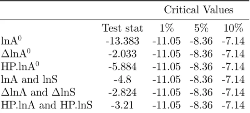
Table 1.2. Tests for unit root - Yearly

Dickey-Fuller test for unit root Phillips-Perron test for unit root H0 RW without drift RW with trend and drift RW without drift RW with trend and drift

lnA0 _0.25 _-2.81 _0.75 _-2.63

(0.97) (0.19) (0.99) (0.27)

lnA0 _-6.81 _-6.85 _-8.99 _-7.02

(0.00) (0.00) (0.00) (0.00)

HP.lnA0 _-6.23 _-6.15 _-6.21 _-6.17

(0.00) (0.00) (0.00) (0.00)

lnA -0.45 -2.52 -0.31 -2.35

(0.90) (0.32) (0.92) (0.40)

lnA -6.80 -6.86 -6.90 -7.20

(0.00) (0.00) (0.00) (0.00)

HP.lnA -6.39 -6.14 -6.46 -6.27

(0.00) (0.00) (0.00) (0.00)

lnS 0.23 -2.38 0.22 -2.42

(0.97) (0.39) (0.97) (0.37)

lnS -6.52 -6.46 -6.52 -6.45

(0.00) (0.00) (0.00) (0.00)

HP.lnS -6.22 -6.15 -6.21 -6.12

(0.00) (0.00) (0.00) (0.00)

Market Return -7.84 -7.75 -7.92 -7.85

(0.00) (0.00) (0.00) (0.00)

Market Return - Risk Free Rate -8.07 -8.07 -8.23 -8.35

(0.00) (0.00) (0.00) (0.00)

This table reports the Dickey-Fuller and Phillips-Perron test statistics (and MacKinnon approximate p-values in parenthesis) of key variables for NYAM stocks constructed with yearly data from January 1961 to December 2011 (50 observations). The table shows test statistics and p-values of the log-transformed Amihud (2002) measure and its stationary transformations. It also shows the test statistics and respective p-values of the turnover version of Amihud (2002) measure and the size variable, including also their starionary versions.

(42)

for lnA0 and 0.01 for HP:lnA0. Figures 4, 5, 6 and 7 show the autocorrelation (ACF) and partial autocorrelation (PACF) functions of lnA0 _and _HP:_ln_A0_{. They show no}

clear indication of the number of AR or MA terms5_.

The …rst PACF is negative and it cuts o¤ after lag 2 (however, it is 5% signi…cant

at lag 22) and the …rst ACF is negative and the only 5% signi…cant point is lag-2. This

suggests that lnA0 may follow an MA(2) process. The autocorrelation and partial autocorrelation functions of the HP-…lteredlnA0 also suggest an MA(2) process.

We observe a similar behavior in the equally weighted series oflnAandlnS. In Table 1.1 we see that the mean (standard deviation) of lnA and lnS are given, respectively, by 2.23 (0.10) and 14.16 (1.23). These variables are also non-stationary, the p-values of

the ADF (Phillips-Perron) tests for unit root are 0.90 (0.92) and 0.97 (0.97) respectively

forlnA and lnS, when we test for a random walk against a stationary AR(1). When we change the underlying model assumption and test for a random walk against a stationary

AR(1) with drift and a time trend, we have p-values of 0.32 (0.40) for the calculated ADF

(Phillips-Perron) statistic of the lnA series and 0.39 (0.37) of the lnS series. We see a decreasing trend on the path oflnA, which is shown in Figure 8, and an upward trend in size, shown in Figure 9.

It is interesting to highlight that, while the peak of illiquidity in the recent years is seen

in 2009 for the original measure, the turnover measure has its peak in 2008. This re‡ects

5_{We can use the rule of thumb to tackle the number of AR or MA terms: if the PACF of the di¤erenced}

(43)

that both measures may have di¤erent sensitivities for what happens in the markets.

Cochrane’s (2005) argument that smaller stocks, which have smaller dollar volume for

the same turnover, are automatically more illiquid for Amihud’s (2002) original measure.

Maybe a decrease of value of large companies lowered the lnA0. However, as lnA takes turnover into account, this measure could capture the drop in illiquidity without the noise

created by …rms’ loss of value.

We also perform the same transformations we use in lnA0 to construct stationary versions of lnA and lnS. The transformed measures are stationary, Table 2 shows that the p-values relative to the ADF and Phillips-Perron tests for the …rst di¤erence and

HP-…ltered variables are all 0.00, rejecting the null hypothesis of unit root.

The nonstationarity of the illiquidity measure is an important point for the estimation

of illiquidity premium. In previous studies this issue is not considered. Amihud’s (2002)

sample ends in 1996 and he does not report any test for unit root/stationarity of illiquidity

in his time-series analysis. Any updated study that measures illiquidity premium over time

should take that into account.

1.4.1.1. Yearly market return. We construct Equally and Value Weighted Market Returns in a way analogous to market illiquidity, however, we just report tables with the

results of the Value Weighted Market Returns, henceforth VWMR, which we denote by

ryM. We also construct the VWMR in excess of the risk-free rate, given by the annualized one-month T-bill rate, which we denote by rE

y. Table 1.1 shows that the values of the means of rM

y andrEy, respectively given by 14.97 and 9.70. Both ADF and Phillips-Perron tests for unit root reject the null hypothesis, at

1% level, that yearly market returns have a unit root. As expected, yearly returns are

stationary. Figures 10, 11, and 12 show, respectively, the path, the ACF, and the PACF

of ryM (the …gures relative to rEy are analogous).

(44)

Yearly market returns do not show any sign of having a structure, all the points in

both of these functions do not seem to be di¤erent from zero (taking Bartlett’s formula

for 95% con…dence bands). In the next subsection we analyze the monthly data in a way

analogous to what we do with yearly data.

1.4.2. Monthly variables

In this subsection we discuss descriptive statistics for monthly data. Table 1.3, analogous

to Table 1.1, reports values of means, medians, standard deviations, and other

descrip-tive statistics for the monthly original Amihud (2002) measure,lnA0, and its stationary transformations.

Table 1.3. Descriptive statistics - Monthly

Variable Obs Mean Std. Dev. Min Max

lnA0 600 -3.24 1.51 -6.31 0.17

lnA0 599 -0.01 0.22 -0.76 1.81

HP.lnA0 600 0.00 0.40 -1.31 1.47

lnA 600 24.28 0.51 23.05 25.69

lnA 599 0.00 0.17 -0.54 0.69

HP.lnA0 600 0.00 0.30 -0.70 1.03

Market Return 600 1.40 4.39 -20.70 18.23

Market Return - Rf 600 0.98 4.39 -21.30 17.72

Market Return - FF3F 600 0.52 4.07 -17.19 16.70

This table reports descriptive statistics of key yearly variables for NYSE-AMEX (hereafter NYAM) stocks from January 1961 to December 2011 (600 months). The table shows statistics for the log-transformed values [indicated by ln(.)] of Amihud (2002) measure and the measures of Return. It also shows statistics for both the log-transformed turnover version of the measure and for the log-transformed size. For each measure we perform two transformations in order to make them station-ary: we take the …rst di¤erence [indicated by (.)] and then apply the …ltering procedure described by Hodrick and Prescott (1981) [denoted by HP.(.)].

There is a total of 600 periods ranging from January 1962 to December 2011. The

mean of the log-transformed VWMI, lnA0_{, is -3.24 over the sample period and its the}

standard deviation is 1.55. Figure 13 plots the path of the monthly lnA0 and it shows that this measure follows a generally decreasing trend.

(45)

During the 1990’s illiquidity decreases steeply. In March and July of 2008 there are

two spikes in illiquidity and after the second one the level of illiquidity remains higher

until August 2009, when it returns to a level close to the one of December of 2007. In

August of 2009 the log of the Amihud measure is -5.33, and in December 2007 it is -5.31.

In between these two periods the mean of the log illiquidity is -4.65.

As in the yearly case, Figure 13 shows a path that can suggest a non-stationary

process. The …rst and third columns of Table 1.4 report the statistics of both the

Aug-mented Dickey-Fuller (ADF) and Phillips-Perron tests for unit root against a stationary

autoregressive process of order one. The ADF statistic (MacKinnon approximate p-values)

of lnA0 is -3.20 (0.02), therefore the null hypothesis of unit root is not rejected at a 1% level, however it is rejected at a 5% level. The Phillips-Perron test yields an statistic of

-1.92 (0.325), which means that the null hypothesis of a unit root is not rejected at any

conventional level.

Columns 2 and 4 of Table 1.4 show the statistics of both the Augmented Dickey-Fuller

(ADF) and Phillips-Perron tests for unit root against a stationary AR(1) with drift and a

time trend. The ADF statistic (MacKinnon approximate p-values) oflnA0 is -8.75 (0.00), therefore the null hypothesis of a unit root is rejected at a 1% level. The Phillips-Perron

test yields an statistic of -8.19 (0.00), which means that the null hypothesis of a unit root

is also rejected at a 1%-signi…cance level.

Taken together, these tests suggest that the lnA0 _{series is trend-stationary. If this is}

the case, we should remove the non-stationarity by detrending. Taking the …rst-di¤erence

also “removes” the non-stationarity but that adds an MA(1) structure into the errors. We

make the same variable transformations we use in the yearly section: (1) we take the …rst

di¤erence of the illiquidity measure ( lnA0) and (2) we use de-trended Amihud’s (2002) original measure using the …lter described by Hodrick and Prescott (1981) (HP:lnA0) with the smoothing parameter set to 129,600, which is the conventional choice.

There are other ways of detrending a series, including simply …tting a linear trend and

(46)

coe¢cient of the trend is -0.0018, and subtract it from the original series. This procedure

yields a stationary series, the Dickey-Fuller test statistic for the detrended series is -4.008,

the related p-value is 0.0014.

The tests for unit root for both the …rst-di¤erenced and the HP-…ltered versions of

lnA0 _{reject the null hypothesis of unit root, as we report in Table 1.4. All the p-values}

of both Augmented Dickey-Fuller and Phillips-Perron tests for all these transformations

are 0.00.

Figures 14 and 15 show the path of these transformed variables, the graphical analysis

also seem to reveal stationary variables. This suggests thatlnA0 calculated with monthly data is integrated of order 1.

The averages of lnA0 and HP:lnA0 are respectively -0.01 and 0.00. As happens with yearly data, their dispersion is high considering their means, the standard deviation

of lnA0 _{is 0.43 and of} _HP:_ln_A0 _{is 0.46.}

Figures 16 and 17 show the autocorrelation and partial autocorrelation functions of

lnA0, …gures 18 and 19 show the same functions of HP:lnA0. The …rst two PAC of

lnA0_{are 5% signi…cant and negative. The …rst ACF is negative 5% signi…cant. The rule}

of thumb would suggest to estimate an ARMA (2,1) speci…cation or at least to consider

some MA structure. However when we use 2 lags in the model, i.e., an AR(2) structure,

the MA term becomes non signi…cant at any conventional level. We test several model

versions and use AIC and BIC statistics as indicators and their lowest values (AIC of

519.24 and BIC of 536.82) are related to the AR(2) model.

(47)

Table 1.4. Tests for unit root - Monthly

Dickey-Fuller test for unit root Phillips-Perron test for unit root

H0 RW without drift RW with trend and drift RW without drift RW with trend and drift

lnA0 _-3.20 _-8.75 _-1.92 _-8.19

(0.02) (0.00) (0.33) (0.00)

lnA0 _-38.11 _-38.08 _-43.87 _-43.86

(0.00) (0.00) (0.00) (0.00)

HP.lnA0 _-12.91 _-12.9 _-13.35 _-13.34

(0.00) (0.00) (0.00) (0.00)

lnA -3.92 -4.55 -3.72 -5.4

(0.00) (0.00) (0.00) (0.00)

lnA -25.75 -25.73 -25.92 -28.68

(0.00) (0.00) (0.00) (0.00)

HP.lnA -7.08 -7.07 -7.18 -8.84

(0.00) (0.00) (0.00) (0.00)

lnS 0.24 -3.52 0.12 -2.05

(0.97) (0.04) (0.97) (0.03)

lnS -22.22 -22.24 -22.30 -22.43

(0.00) (0.00) (0.00) (0.00)

HP.lnS -6.12 -6.11 -6.76 -5.74

(0.00) (0.00) (0.00) (0.00)

Market Return -22.99 -22.97 -22.97 -22.97

(0.00) (0.00) (0.00) (0.00)

Market Return - Risk Free Rate -22.95 -22.96 -22.93 -22.94

(0.00) (0.00) (0.00) (0.00)

Market Return - FF3 adjusted -24.12 -24.19 -24.15 -24.21

(0.00) (0.00) (0.00) (0.00)

This table reports the Dickey-Fuller and Phillips-Perron test statistics (and MacKinnon approximate p-values in parenthesis) of key variables for NYAM stocks constructed with monthly data from January 1961 to December 2011 (600 observations). The table shows test statistics and p-values of Returns and the log-transformed Amihud (2002) measure, including its stationary transformations. It also shows the test statistics and respective p-values of the turnover version of Amihud (2002) measure and the size variable, as well as their starionary versions.

(48)

The ACF of HP:lnA0 decrease exponentially until the 9th lag, and the PACF cuts o¤ after the 2nd lag. It seems that and ARMA with enough lags can capture the dynamic of

this variable, we test several lags combinations using AIC and BIC as comparison criteria.

The lowest AIC and BIC, 466.60 and 488.58 respectively, are achieved when we estimate

an ARMA (2,2).

The Equally Weighted Market Illiquidity using the turnover version of Amihud (2002)

measure calculated with monthly data is harder to analyze. Figures 20 show the path

of this variable, it seems to have a decreasing trend but it is not as clear as the yearly

counterpart.

As we show in Table 4, both ADF and Phillips-Perron tests reject the hypothesis

of unit root at a 1%-level when we do not control for serial correlation of this series.

Figure 21 shows the autocorrelation function of lnA, we see that it dumps out close to the 20th lag (which looks like a non-stationary process). We run the ADF test allowing

the autocorrelation up to the 20th lag and it yields a calculated statistic (p-value) of -2.71

(0.07). It rejects the null hypothesis of the existence of a unit root at a 10%-level.

The results in Table 1.4 also show that the …rst-di¤erence of lnA and the HP-…ltered transformation are stationary as all of the calculated statistics of both ADF and

Phillips-Perron tests reject the null hypothesis of existence of unit root at a 1%-level. We must also

access the properties of the log-transformed size, as this variable is one of the components

of the turnover version of Amihud (2002). The log-transformed size seem to be

non-stationary, the p-values of both the Augmented Dickey-Fuller and Phillips-Perron tests

for unit root are 0.97. Figure 22 shows the path oflnS which has an upward trend.

(49)

cointegrate and for monthly data they do seem to have a cointegration relation, therefore,

we can use an Autoregressive Distributed Lag (ARDL) speci…cation to estimate the model.

So far we have focused on the monthly illiquidity, in the next subsection we focus on the

description of monthly returns.

1.4.2.1. Monthly market return. We construct both equally and value weighted mar-ket returns but throughout the text we just show the results for the Value Weighted

Mar-ket Return (VWMR). Once the average of cross-sectional returns is calculated for each

period, we make two adjusts: (1) we subtract the risk-free rate, given by the one-month

T-bill rate of each market return getting the return in excess of the risk-free rate, and; (2)

we use Fama and French’s (1993) Three Factors (FF3F) to adjust returns. These adjusts

yields three market return variables for monthly data.

We denote the value VWMR in monthmbyrM

m and the return in excess of the monthly risk-free rate by rEm. We de…ne the additional measure, representing the market return in excess of the Fama and French (1993) three factors. The construction of this variable

requires the estimation of the factor loadings, what we do using the entire sample period.

Letri;m denote the return of …rm i’s stock on monthm; and rfm denote the risk-free rate of return for month m, given by the return on the one month T-Bill. We estimate the following model

(1.37) ri;m rmf =ai+bi;1M KT +bi;2SM B+bi;3HM L+"t

whereM KT can be de…ned as the VWMR in month m; SM B stands for "Small Minus Big" andHM Lstands for "High Minus Low" which are calculated after forming 6 portfo-lios using market capitalization and book-to-market ratio. The resulting FF3F-adjusted

excess return, denoted byrF F3

i;m for stockiin each monthm;is calculated as the sum of the intercept and the residual from time-series regressions in which the dependent variable is

the stock return in excess of the one-month T-bill rate. Then the FF3-adjusted returns

Essays on illiquidity premium

List of Tables

Contents

Introduction

Abstract