Model Reduction-Based Control of the Buck Converter Using Linear Matrix Inequality and Neural Networks

Model Reduction-Based Control of the Buck Converter Using Linear Matrix

Inequality and Neural Networks

Anas N. Al-Rabadi and Othman M.K. Alsmadi

Abstract - A new method to control the Buck converter using new small signal model of the pulse width modulation (PWM) switch is introduced. The new method uses recurrent supervised neural network to estimate certain parameters of the transformed system matrix [ A~]. Then, linear matrix inequality (LMI) optimization is used to obtain the permutation matrix [P] so that system transformation {[B~], [ C~], [E~]} is achieved. The transformed model is then reduced using the singular perturbation method, and state feedback control is applied to enhance system performance. The eigenvalues of the resulting transformed reduced model are an exact subset of the original (non-transformed full-order system), and this is important since the eigenvalues in the non-transformed reduced order model will be different from the eigenvalues of the original full-order system. The experimental simulation results show that the new control method simplifies the model in the Buck converter and thus uses a simpler controller that produces the desired system response for performance enhancement.

Index Terms _{- Buck Converter, Feedback Control, Linear} Matrix Inequality (LMI), Neural Network, Order Model Reduction, Supervised Learning.

1.

INTRODUCTION

Recently, small-signal modeling of dynamic behaviors of the open loop dc-to-dc power converters has attracted much attention, due to the fact that these models are the basis to extract accurate transfer functions [1,6], which are essential in the feedback control design. They are used to design reliable high performance regulators, by enclosing the open loop dc-to-dc power converters in a feedback loop, to keep the performance of the system as close as possible to the desired operating conditions, and to counteract the outside disturbances [7,13].

These power converters usually work in the Continuous Conduction Mode (CCM), or in the Discontinuous Conduction Mode (DCM) [1,6]. The CCM mode is desirable, as the output ripple of the dc-to-dc power converter is very small compared to the dc steady state output. A linearized small-signal model is constructed to examine the dynamic behaviors of the converter, due to the fact that these disturbances are of small signal variations. Through this model, the necessary open-loop transfer functions can be determined and plotted using Bode plots [6]. This is needed in order to use compensation to the pulse width modulation (PWM) power converters, to meet the desired nominal operating

A. N. Al-Rabadi is with the Computer Engineering Department, The University of Jordan, Amman, Jordan (Phone: + 962-79-644-5364; E-mail: alrabadi@yahoo.com; URL: http://web.pdx.edu/~psu21829/) O. M.K. Alsmadi is with the Electrical Engineering Department, The University of Jordan, Amman, Jordan (E-mail: othman_mk@yahoo.com)

conditions, through applying various control techniques. These control methods use the approaches of: frequency analysis in the classical control theory, time analysis in the modern control theory, both frequency analysis and time analysis domains in the post modern (digital and robust) control theory, and soft computing (fuzzy logic (FL) + neural networks (NN) + genetic algorithms (GA)) in the intelligent control theory [6,7,13,16,17]. These control methods can be applied to the models of power converters that usually work with only one specific control scheme; pulse width modulation (PWM) through either duty-ratio control or current programming control [6]. The converter modeling approaches utilize in general four techniques [1,6]: (1) the sampled-data technique, (2) the averaged technique, (3) the exact small-signal analysis technique, and (4) the combination of the averaged technique and the sampled-data technique. A new small-signal modeling approach which is applicable to any power converter system represented as a two-port network has been introduced [1]. This was done through the modeling of the nonlinear part in the power converter system, which is the PWM switch.

In system modeling, sometimes it is required to identify some parameters, and this can be achieved by using artificial neural networks (ANN). Artificial neural systems can be defined as cellular systems which have the capability of acquiring, storing, and utilizing experiential knowledge [17]. They can be used to model complex relationships between inputs and outputs or to find patterns in data. An ANN consists of an interconnected group of artificial neurons and processes information using a connectionist approach to computation. The basic processing elements of neural networks are called neurons, which perform summing operations and nonlinear function computations. Neurons are usually organized in layers and forward connections. Computations are performed in parallel at all nodes and connections. Each connection is expressed by a numerical value called a weight. The learning process of a neuron corresponds to a way of changing its weights [4,10,16,17].

When dealing with system modeling and control analysis, some equations and inequalities need optimized solutions. A numerical algorithm, used in robust control called linear matrix inequality (LMI) serves as a source of application problems in convex optimization [5]. LMI optimization method started by the Lyapunov theory showing that the differential equation x&(t)=Ax(t) is stable iff there exists a positive definite matrix [P] such that

0

< +PA P

the linear equation ATP+PA=−Qfor [P], it is guaranteed that [P] is positive-definite if the given system is stable.

Usually in practical control problems, the first step is to obtain a mathematical model in order to examine the behavior of the system for the purpose of designing a suitable controller [7]. In some systems, this mathematical description involves a certain small parameter (perturbation). Neglecting this small parameter results in simplifying the order of the designed controller based on reducing the order of the system model (method of singular perturbation) [2,8,12,14,15]. This simplification and reduction of system modeling leads to controller cost minimization [12].

Figure 1 presents the layout of the Buck-based converter new control methodology used in this paper.

State Feedback Control Order Model Reduction

System Transformation: {[B~], [C~], [E~]} LMI-Based Permutation Matrix: [P] System Undiscretization (Continuous) Neural-Based State Transformation: [A~]

System Discretization

New Model of Buck Converter: {[A], [B], [C], [E]}

Figure 1. Buck converter new hierarchical control methodology introduced in this paper.

2. BACKGROUND

This section presents important background on Buck converter, supervised neural network, LMI, and order model reduction that will be used in Sections 3, 4 and 5. 2.1The Application of the New Small Signal

Model on the PWM Converters

There are several averaged modeling techniques used to model the PWM converters. These techniques include: volt-second and current-second balance approach, and the state-space averaging approach [1,6]. These techniques are used to model the converter systems as a whole, as well as to model the pulse width modulation (PWM) switch by itself. These methods are accurate for the low frequency range, but inaccurate in the high frequency range [6]. Another modeling approach that focuses on modeling the converter-cell, instead of the converter as a whole, is used to get averaged models for the PWM converters. This approach is also useful for the low frequency ranges, but not useful for the high frequency ranges. One major advantage of these techniques is the fact that they are easy to implement and the results derived are not in complicated forms.

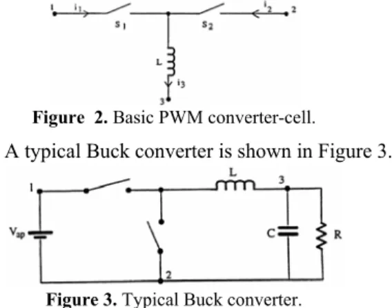
The averaged modeling approach aims to produce an averaged model for a specific cell of the PWM converters. This cell is shown in Figure 2, where this basic cell is used to explore the dc behaviors and the ac small- signal dynamic behaviors of the PWM Buck converter.

Figure 2. Basic PWM converter-cell.

A typical Buck converter is shown in Figure 3.

Figure 3. Typical Buck converter.

It's been shown in [1] that a new small-signal model of the PWM switch can be as shown in Figure 4, where:

L jD T

j e L T

T D j e DT j e DT j DT j T j e h

2

) s 1 ( 2 s

s s

s 1 ) s 1 ( s

1 _{ω ω}

ω

ω ω

ω ω

ω

+ −

−

− − − − − + + −

= '

) s 1 (

) s 1

( s

2 _{j T}

e L

p Va DT j e T D j je L

p jDVa Ix

h _ω

ω

ω ω

ω ₋ −

− − −

− +

= '

Figure 4. New small-signal model of the PWM switch. The new switch model shown in Figure 4, is an exact small-signal model, since the mathematical equations upon which the whole derivation process was built, are exact [1]. Also, we note that two of the dependent current sources are frequency dependent, which is uncommon for current or voltage dependent sources.

2.1.1 Applying the PWM New Small Signal Model in the Buck Converter

In this subsection, the new small-signal model of the PWM switch will be investigated on the PWM Buck converter. The control-to-output and input-to-output transfer functions will be derived for the Buck converter using the new small-signal model of the PWM switch. These transfer functions will be compared to the corresponding transfer functions for the averaged modeling approach and the exact model of the Buck converter.

By applying the PWM switch model, that was developed previously on the Buck converter, one obtains the equivalent circuit model as shown in Figure 5, where we assume that the input dc voltage source Vg has small

signal perturbation

v

ˆ

_g and that: |V_g |>>|vˆ_g |.

In Figure 5, the output equation isy=vˆo =vˆc.

0 k

w

1 k

w

2 k

w

∑

()

•

ϕ yk

1

x

p

x

Output Activation Function

Summing Junction

Synaptic Weights Input

Signals

k

v

Threshold k kp

w

0

x

2

x

Figure 5. Circuit model of the PWM Buck converter obtained through applying the new PWM switch small signal model.

{x ₌

⎥ ⎥ ⎦ ⎤ ⎢ ⎢ ⎣ ⎡

o l v

i ˆ ˆ

, u _{= ⎥}

⎦ ⎤ ⎢ ⎣ ⎡

d v_g ˆ ˆ

}, the system quadruple {[A],[B],[C],[E]} will be [1]:

⎥ ⎦ ⎤ ⎢

⎣ ⎡

− − =

1/RC 1/C

1/L 0

A , _⎥

⎦ ⎤ ⎢

⎣ ⎡ =

0 0

/L V D/L g

B ,

T

C _⎥

⎦ ⎤ ⎢ ⎣ ⎡ =

1 0

,

T

E _⎥

⎦ ⎤ ⎢ ⎣ ⎡ =

0 0

To find the control-to-output transfer function, we null the input

v

ˆ

_g. The new system quadruple {[A],[B],[C],[E]}, will be [1]:

A = _⎥

⎦ ⎤ ⎢

⎣ ⎡

− − 1/RC 1/C

1/L 0

, B = _⎥

⎦ ⎤ ⎢ ⎣ ⎡

0

/L Vg

,

T

C _⎥

⎦ ⎤ ⎢ ⎣ ⎡ =

1 0

, E =

[ ]

0 In order to find the control-to-output transfer

function from the system quadruple, we apply the Laplace transformation to both sides of the state and the output equations represented by system state space equations:

) ( ) ( )

(t Axt But

x& = + and y(t)=Cx(t)+Eu(t). After

re-arranging terms, the following input-to-output transfer function is obtained [1,6]:

C s A B E

u

y _{= −} −1 ₊

)

( Ι (1) By applying the above system quadruple in Equation (1) for the circuit values of {Vg = 15 V, R = 18.6

Ω , D = 0.4, fs = 40.3kHz, D´ = 0.6, L = 58 µH, C = 5.5 µF}, and to investigate the accuracy of the new PWM switch model, one refers to Figure 6.

Figure 6. The control-to-output frequency response of the PWM Buck converter, operating in CCM: exact (solid line); averaged (dotted line); and the new model (dashed line).

To get the input-to-output transfer function, we null the input dˆ. The system quadruple {[A],[B],[C],[E]} will be [1]:

A = _⎥

⎦ ⎤ ⎢

⎣ ⎡

− − 1/RC 1/C

1/L 0

, B = _⎥

⎦ ⎤ ⎢ ⎣ ⎡

0 D/L

, C =

[

0 1

]

, E =

[ ]

0 By applying the above system quadruple in Equation (1) for the circuit values of {Vg = 15V, R = 18.6

Ω , D = 0.4, fs = 40.3kHz, D´ = 0.6, L = 58 µH, C = 5.5

µF}, and to investigate the accuracy of the new PWM switch model, one refers to Figure 7.

Figure 7. The input-to-output frequency response of the PWM Buck converter, operating in CCM: exact (solid line); averaged (dotted line); and the new model (dashed line).

From the above frequency response plots for both control-to-output and input-to-output transfer functions of the PWM Buck converter, operating in the CCM, we observe that an excellent match occurs between the exact and the new model results, as well as between the averaged and the new model results [1].

2.2 Recurrent Supervised Neural Computing An artificial neural network (ANN) is an emulation of a biological neural system [17], where the basic model of the neuron is based on the functionality of a biological neuron which is the basic signaling unit of the nervous system. A model of a neuron is shown in Figure 8.

Figure 8. A neuron mathematical model.

From Figure 8, the internal activity of a neuron is:

∑

=

=

p

j

j kj

k w x

v

1

(2) In supervised learning, it is assumed that, at each time instant when the input is applied, the desired response of the system is available [2,4,10,16,17]. The difference between the actual and desired responses represents an error measure which is used to correct the network parameters. The weights have initial values and the error measure is used to adapt the network's weight matrix [W]. A set of input and output patterns, called the training set, is needed for this learning. A training algorithm estimates the directions of the negative error gradient and reduces the resulting error accordingly [17].

Z-1 g1:

A11 A12

A21 A22 B11 B21 ) 1 ( ~

1 k+

x System external input System dynamics System state: internalinput Neuron delay Z-1 Outputs ~y(k)

) 1 ( ~

2 k+

x

) ( ~

1k

x ~x2(k)

4

4 8

4

4 7

6

of steepest descent [16,17]. The network tries to match the actual output of certain neurons to the target values at specific instant of time. Consider a NN consisting of a total of N neurons with M external input connections, as shown in Figure 9, for a 2nd order system with two neurons and one external input.

Figure 9. A 2nd order recurrent NN architecture whith the

estimated matrices given by { _⎥

⎦ ⎤ ⎢ ⎣ ⎡ = ⎥ ⎦ ⎤ ⎢ ⎣ ⎡ = 21 11 22 21 12

11 _,~

~ B B B A A A A

A_{d d} },

where W =

[

[A~_d] [~B_d]

]

.

The variable g(k) denotes the (M x 1) external input vector applied to the NN at discrete time k. The variable y(k + 1) denotes the corresponding (N x 1) vector of individual neuron outputs produced at time (k + 1). The input vector g(k) and the one-step delayed output vector

y(k) are concatenated to form the ((M + N) x 1) vector

u(k), whose ith element is denoted by ui(k). IfΛ denotes

the set of indices i for which gi(k) is an external input,

and

ß

denotes the set of indices i for which ui(k) is the

output of a neuron (which is yi(k)), then:

⎪⎩ ⎪ ⎨ ⎧ ∈ ∈ β i , k y Λ i , k g = k u i i i if ) ( if ) ( ) (

The (N x (M + N)) weight matrix of the recurrent NN is represented by [W]. The net internal activity of neuron j at time k is given by:

∑

∪ ∈ = β Λ i i ji

j k w k u k

v ( ) ( ) ( )

At time (k + 1), the output of the neuron j is computed by: yj(k+1)=ϕ(vj(k))

The derivation of the recurrent algorithm starts by using dj(k) to denote the desired (target) response of

neuron j at time k, and

ς

(k)

to denote the set of neurons that are chosen to provide externally reachable outputs. A time-varying (N x 1) error vector e_{(k) has a j}th _element given by: ⎪⎩ ⎪ ⎨ ⎧ ∈ otherwise 0, ) ( if ), ( -) ( = ) ( k j k y k d k

e_j j j

ς

The objective is to minimize the cost function Etotal as:

E_total= E(k)

k

∑

, where ( )

2 1 = )

(k e2 k

E _j

j

∑

∈ς

To accomplish this, the method of steepest descent which requires knowledge of the gradient matrix is used:

total= total = ( )= E(k)

k E E E k k W W W

W ∂ ∇

∂ ∂

∂

∇

∑

∑

where∇WE(k) is the gradient of E(k) with respect to the weight matrix [W]. In order to train the recurrent NN in real time, the instantaneous estimate of the gradient is used

(

∇WE(k)

)

. For a particular weight

w

ml(k), the

incremental change Δw_ml(k) at time k is defined as: ) ( ) ( -= ) ( k w k E k w m m l l _∂ ∂ Δ η

where is the learning-rate parameter. Hence: ) ( ) ( ) ( -= ) ( ) ( ) ( = ) ( ) ( k w k y k e k w k e k e k w k E m i j j m j j j

ml l ∂ l

∂ ∂ ∂ ∂ ∂

∑

∑

∈

∈ς ς

To determine the partial derivative

) ( )/ (k w k yj ∂ ml

∂ , the NN dynamics are derived. The

derivation is obtained by using the chain rule as follows: ) ( ) ( )) ( ( = ) ( ) ( ) ( 1) + ( = ) ( 1) + ( k w k v k v k w k v k v k y k w k y m j j m j j j m j l l l & ∂ ∂ ∂ ∂ ∂ ∂ ∂ ∂ ϕ , where ) ( )) ( ( = )) ( ( k v k v k v j j j _∂ ∂ϕ

ϕ& . Differentiating the net

internal activity of neuron j with respect to

w

_ml(k) yields:

⎥ ⎥ ⎦ ⎤ ⎢ ⎢ ⎣ ⎡ ∂ ∂ ∂ ∂ ∂ ∂ ∂ ∂

∑

∑

∪ ∈ ∪ ∈ ) ( ) ( ) ( + ) ( ) ( ) ( = ) ( )) ( ) ( ( = ) ( ) ( k u k w k w k w k u k w k w k u k w k w k v i m ji m i ji Λ i m i ji Λ i m j l l l l β β

where

(

∂w_ji(k)/∂w_ml(k)

)

equals "1" only when j = m and

i = l, otherwise it is "0". Thus:

δ u (k)

(k) w (k) u k w k w k v mj m i ji Λ i m j l l l + ∂ ∂ ∂ ∂

∑

∪ ∈ ) ( = ) ( ) ( β

where δmj is a Kronecker delta equal to "1" when j = m

and "0" otherwise, and: ⎪ ⎩ ⎪ ⎨ ⎧ ∈ ∂ ∂ ∈ ∂ ∂ β i k w k y Λ i k w k u m i m i if , ) ( ) ( if 0, = ) ( ) ( l l

Having these equations provides that:

⎥ ⎥ ⎦ ⎤ ⎢ ⎢ ⎣ ⎡ + ∂ ∂ ∂ ∂

∑

∈ ) ( ) ( ) ( ) ( )) ( ( = ) ( 1) + ( k u k w k y k w k v k w k y m m i ji i j m j l l l l & _δ ϕ β

with =0

) 0 ( (0) l m i w y ∂ ∂

B

∫

C D

A +

+

+ y(t)

u(t) x&(t) x(t)

+

The dynamical system is described by the following triply indexed set of variables (

π

_mj_l):

) (

) ( = ) (

k w

k y k

m j j

m

l

l _∂

∂

π

For every time step k and all appropriate j, m and

l, system dynamics (with π_mj_l(0)=0) are controlled by:

⎥ ⎥ ⎦ ⎤ ⎢

⎢ ⎣ ⎡

+

∑

∈

) ( )

( ) ( ))

( ( = 1) +

(k v k wji k mi k mju k

i j j

ml ϕ& π l δ l

π

β

The values of π_mj_l(k) and the error signal ej(k) are

used to compute the corresponding weight changes: w (k)= ej(k) mj (k)

j

m η π

ς l

l

∑

∈

Δ (3)

Using the weight changes, the updated weight

l m

w (k + 1) is calculated as follows:

w_ml(k+1)=w_ml(k)+Δw_ml(k) (4) Repeating the upper computation, the cost function is minimized and the objective is achieved.

2.3 LMI and Model Transformation

In this section, the detailed process of system transformation using LMI optimization will be presented. Consider the following system:

x&(t)=Ax(t)+Bu(t) (5) y(t)=Cx(t)+Eu(t) (6) The state space representation of Equations (5) and (6) is described as shown in Figure 10.

Figure 10. State space block diagram.

To determine the transformed matrix [A], which is [A~ ], the discrete zero input response is obtained. This is achieved by providing the system with some initial state values and setting the system input to zero (u(k) = 0). Hence, the discrete system of Equations (5) and (6), with the initial condition x(0)=x₀, becomes:

x(k+1)=Adx(k) (7)

y(k)=x(k) (8) We need x(k) as a target to train the NN to obtain the needed parameters in [Ad

~

] such that the system output will be the same for [Ad] and [Ad

~

]. Hence, simulating this system (in Equations (7) and (8)) provides the state response with only [Ad] being used. Once the

input-output data is obtained, transforming the [Ad] is

achieved using the NN training, as explained in Section 3.

The estimated transformed [Ad] matrix is then converted

back into the continuous form which yields:

_⎥

⎦ ⎤ ⎢

⎣ ⎡ =

o c r

A A A A

0 ~

(9) Having the continuous [A] and [A~ ] matrices, the permutation [P] matrix is determined using the LMI optimization technique, as will be illustrated in later sections. The complete system transformation can be obtained as follows: assuming that x~=P−1x, the system of Equations (5) and (6) can be re-written as:

P~x&(t)=AP~x(t)+Bu(t), ~y(t)=CP~x(t)+Eu(t)

Pre-multiplying the state equation by [P-1], we obtain: P−1P~x&(t)=P−1AP~x(t)+P−1Bu(t) which yields the following transformed model:

x~&(t)=A~~x(t)+B~u(t) (10) ~y(t)=C~~x(t)+E~u(t) (11) where the transformed system matrices are given by {A~=P−1AP,B~=P−1B,C~=CP,E~=E}. Transforming the system matrix [A] into the form shown in Equation (9) can be achieved based on the following definition [11].

Definition.Matrix A∈M_nis called reducible if either: (a) n = 1 and A = 0; or

(b) n≥ 2, there is a permutation matrix P∈M_n, and there is some integer r with1≤r≤(n−1) such that:

_⎥

⎦ ⎤ ⎢ ⎣ ⎡ =

−

Z Y X AP P

0 1

(12) where X∈M_r,r, Z∈M_n−r,n−r, Y∈M_r,n−r, and

0∈M_n−r,r is a zero matrix.

The attractive features of the permutation matrix [P] such as being orthogonal and invertible have made this transformation easy to implement. However, the permutation matrix structure narrows the applicability of this method to a very limited category of applications. Some form of a similarity transformation maybe used to correct this problem; f :Rn×n →Rn×n, where f is a linear operator defined by f(A)=P−1AP [11]. Hence, based on the [A] and [A~], LMI is used to obtain [P]. The optimization problem is casted as follows:

P−P_o Subjectto P− AP−A <ε P

~

min 1 (13)

which maybe written in an LMI equivalent form as:

0 )

~ (

~

0 )

( )

( min

1

1 2

1 _>

⎥ ⎥ ⎦ ⎤ ⎢

⎢ ⎣ ⎡

−

− > ⎥ ⎦ ⎤ ⎢

⎣ ⎡

−

−

−

−

I A

AP P

A AP P I

I P P

P P S to Subject S trace

T T o

o S

ε (14)

where S is a symmetric slack matrix [5]. 2.4 Order Model Reduction

0 0.1 0.2 0.3 0.4 0.5 0.6 0.7 0.8 0.9 1 0 0.01 0.02 0.03 0.04 0.05 0.06 0.07 0.08 0.09 Time[s] S y s tem O u tp ut + - 1 L 1 R out

v

a b in

v

2

L L3

1

C C2 R2

+ - + - 1 x 2 x 3 x 4 x 5 x

singularly perturbed systems [2,12]. Neglecting the fast dynamics of a singularly perturbed system provides a reduced order system model, which has the advantage of designing simpler lower-dimensionality order controllers.

To show the development of a reduced order model, consider the singularly perturbed system [2]: x&(t)=A₁₁x(t)+A₁₂ξ(t)+B₁u(t), x(0)=x₀ (15) εξ&(t)= A₂₁x(t)+A₂₂ξ(t)+B₂u(t), ξ(0)=ξ₀ (16) y(t) =C₁x(t)+C₂ξ(t) (17) where_x∈ℜm1 _and ξ∈ℜm2 _{are the slow and fast state} variables, respectively, _u∈ℜn1 _{and y}∈ℜn2_{are the input} and output vectors, respectively, {[Aii], [Bi], [Ci]} are

constant matrices of appropriate dimensions with

} 2 , 1 { ∈

i , and

ε

is a small positive constant. The singularly perturbed system in Equations (15)-(17) is simplified by setting ε=0 [2,3,12], in which we are neglecting the fast dynamics of the system and assuming that the state vector

ξ

has reached the quasi-steady state. Hence, setting ε=0 in Equation (16), with the assumption that [A22] is nonsingular, produces:

() () 1 ()

1 22 21

1

22A x t A Bu t A

t =− − _r − −

ξ (18)

where the index r denotes remained or reduced model. Substituting Equation (18) in Equations (15)-(17) yields the following reduced order model:

x&_r(t) =A_rx_r(t)+B_ru(t) (19) y(t)=C_rx_r(t)+E_ru(t) (20) where:

21

1 22 12

11 A A A

A

Ar = − − (21)

2

1 22 12

1 A A B

B

B_r = − − (22)

21

1 22 2

1 C A A

C

Cr = − − (23)

2

1 22 2A B C

E_r =− − (24)

Example 1. Consider the following 2nd order system:

() 1 1 ) ( 40 8 15 30 )

(t xt ut

x _⎥ ⎦ ⎤ ⎢ ⎣ ⎡ + ⎥ ⎦ ⎤ ⎢ ⎣ ⎡ − − =

& , y(t)=

[ ]

1 1x(t)

This 2nd order system is overdamped since the two eigenvalues are distinct negative real numbers: {-22.9584, -47.0416}. As seen from the eigenvalues, since there are two distinct categories (fast and slow) with big difference between them, the singular perturbation technique can be applied. The reduced 1st order model is obtained as:

x&_r(t)=−27x_r(t)+1.375u(t)

y_r(t)=1.2x_r(t)+0.025u(t)

As seen in Figure 11, the singular perturbation reduction has provided an acceptable response when compared with the original response.

Example 2. Consider the 5th order RLC filter shown in Figure 12 [9]. It is well known that the capacitor and the inductor are dynamical passive elements leading to their ability to store energy. The dynamical equations are derived using the Kirchhoff's current law (KCL) and Kirchhoff's voltage law (KVL) [9]. The capacitor current

Figure 11. Output step response of the original and reduced order models ( ___ original model, -.-.-. reduced model).

is proportional to the change of its voltage as follows: dt t dv C t i i i c i c ) ( ) ( =

and the inductor voltage is proportional to the change of its current obtained as follows:

dt t di L t v i i L i L ) ( ) ( =

Figure 12. A 5th order RLC-based network (circuit). In order to obtain a state space model, let the system dynamics be the system states (x_i). This means that this is a 5th order system since it contains five dynamical elements. Applying KCL at nodes (a) and (b) and KVL for the three loops starting from left to right in Figure 12, the following state equations are:

) ( 1 ) ( 1 ) ( ) ( 1 2 1 1 1 1

1 _L x t _L x t _Lv t

R t

x& =− − + _in , () 1 () 1 ₃() 1 1 1

2t _C x t _C x t

x& = −

) ( 1 ) ( 1 ) ( ₄ 2 2 2

3t _L x t _L x t

x& = + , () 1 () 1 ₅() 2 3 2

4t _C x t _C x t

x& = − ,

) ( ) ( 1 ) ( ₅ 3 2 4 3

5 _L x t

R t x L t

x& = −

Hence, the system may be given by:

x&(t)=Ax(t)+Bu(t), y(t)=Cx(t)+Eu(t), where:

⎥ ⎥ ⎥ ⎥ ⎥ ⎥ ⎥ ⎥ ⎥ ⎥ ⎥ ⎥ ⎥ ⎦ ⎤ ⎢ ⎢ ⎢ ⎢ ⎢ ⎢ ⎢ ⎢ ⎢ ⎢ ⎢ ⎢ ⎢ ⎣ ⎡ − − − − − − = 3 2 3 1 0 0 0 2 1 0 2 1 0 0 0 2 1 0 2 1 0 0 0 1 1 0 1 1 0 0 0 1 1 1 1 L R L C C L L C C L L R A , ⎥ ⎥ ⎥ ⎥ ⎥ ⎥ ⎥ ⎦ ⎤ ⎢ ⎢ ⎢ ⎢ ⎢ ⎢ ⎢ ⎣ ⎡ = 0 0 0 0 1 1 L B , T R C ⎥ ⎥ ⎥ ⎥ ⎥ ⎥ ⎦ ⎤ ⎢ ⎢ ⎢ ⎢ ⎢ ⎢ ⎣ ⎡ = 2 0 0 0 0

,E=

[ ]

0

Given the values {C₁=2.57nF, C₂ =2.57nF,

H 9.82

1= μ

L , L₂ =31.8μH, L₃ =9.82μH,

Ω = = ₂ 100

1 R

0 0.5 1 1.5 2 2.5 3 x 10-6 0

0.1 0.2 0.3 0.4 0.5 0.6 0.7

Time(secs)

S

y

s

te

m

O

u

tp

u

t

obtained. The eigenvalues of the system are

) 7029 . 3 0865 . 5 , 2839 . 6 , 9863 . 5 9445 . 1 (

106× − ±j − − ±j . Performing

model reduction, the system is reduced to 4th order by taking the first four rows of [A] as the first category represented by Equation (15) and taking the fifth row of [A] as the second category represented by Equation (16). Simulations of the original and the reduced models are shown in Figure 13.

Figure 13. System output step response of the original and reduced order models ( ___ original model, -.-.-reduced model).

3. NEURAL PARAMETER ESTIMATION WITH LMI OPTIMIZATION FOR THE BUCK MODEL REDUCTION

Our objective is to search for a similarity transformation to decouple a pre-selected eigenvalue set from the system matrix [A]. To achieve this objective, training the NN to estimate the transformed discrete system matrix [Ad

~

] is performed [16,17]. For the system of Equations (15)-(17), the discrete model of the Buck converter is obtained as: x(k+1)=A_dx(k)+B_du(k) (25) y(k)=C_dx(k)+E_du(k) (26) The estimated discrete model of Equations (25)-(26) can be written in a detailed form as:

( )

) ( ~

) ( ~ )

1 ( ~

) 1 ( ~

21 11

2 1

22 21

12 11

2 1

k u B B k x

k x A A

A A k

x k x

⎥ ⎦ ⎤ ⎢ ⎣ ⎡ + ⎥ ⎦ ⎤ ⎢ ⎣ ⎡ ⎥ ⎦ ⎤ ⎢

⎣ ⎡ = ⎥ ⎦ ⎤ ⎢

⎣ ⎡

+ +

(27)

_⎥

⎦ ⎤ ⎢ ⎣ ⎡ =

) ( ~

) ( ~ ) ( ~

2 1

k x

k x k

y (28)

where k is the time index. The detailed matrix elements of Equations (27) and (28) are shown in Figure 9.

The recurrent NN can be described by defining Λ as the set of indices i for which g_i(k)is an external input which in the Buck converter system is one external input, and by defining ß as the set of indices i for which yi(k)is

an internal input or a neuron output which in the Buck converter system is two internal inputs (i.e., two system states). Also, we define ui(k)as the combination of the

internal and external inputs for which i∈ß∪Λ. Using this setting, training the NN depends on the internal activity of each neuron which is given by:

∑

∪ ∈ =

β Λ i

i ji

j k w k u k

v ( ) ( ) ( ) (29)

where wji is the weight representing an element in the

system matrix [A~d]or input matrix ] ~

[Bd for {j∈ß,

∪ ∈ß

i Λ} such that W =

[

[A~d] [B~d]

]

. At (k +1), the

output (internal input) of the neuron j is computed by: x_j(k+1)=ϕ(v_j(k)) (30)

Based on an approximation of the method of steepest descent, the NN estimates the system matrix [Ad]

in Equation (7) for zero input response [17]. The error is obtained by matching the true state output with the neuron output as:

e_j(k)=x_j(k)−x~_j(k)

The objective is to minimize the cost function given by: =

∑

k k E

E_total ( ), where

∑

∈ =

ς j

j k e k

E( ) ₂1 2( )

where

ς

denotes the set of indices j for the output of the neuron structure. This cost function is minimized by estimating the instantaneous gradient of E(k) with respect to the weight matrix [W] and then updating [W] in the negative direction of this gradient [16,17]. This is performed as follows:

- Initialize [W] by a set of uniformly distributed random numbers. Starting at the instant k = 0, use Equations (29) and (30) to compute the output values of the N neurons (whereN = ß).

- For every time step k and { j∈ß, m∈ß,l∈ß∪Λ} compute the dynamics of the system governed by the triply indexed set of variables:

⎥ ⎥ ⎦ ⎤ ⎢

⎢ ⎣ ⎡

+ =

+

∑

∈ß i

mj i

m ji j

j

ml(k 1) ϕ&(v (k)) w (k)π l(k) δ ul(k)

π

with initial conditions π_mj_l(0)=0, andδ_mj is given by

(

∂w_ji(k) ∂w_ml(k)

)

which is equal to "1" only when {j = m, i=l} otherwise it is "0". Note that for the special case of a sigmoidal nonlinearity in the form of a logistic function, the derivative ϕ&(

⋅

) is:

ϕ&(vj(k))=yj(k+1)[1−yj(k+1)]

- Compute the weight changes corresponding to the error signal and system dynamics as:

∑

∈

= Δ

ς π η

j

j m j

m k e k k

w _l( ) ( ) _l( ) (31) - Update the weights in accordance with:

0 0.2 0.4 0.6 0.8 1 1.2 1.4 1.6 1.8 2 0

0.05 0.1 0.15 0.2 0.25 0.3 0.35 0.4

Time[s]

S

y

s

te

m

O

u

tp

u

t

0 0.01 0.02 0.03 0.04 0.05 0.06 0.07 0.08 0.09 0.1

0 0.05 0.1 0.15 0.2 0.25 0.3 0.35 0.4 0.45 0.5

Time[s]

S

y

s

tem

O

ut

put

matrix [A~]. Using the LMI optimization technique presented in Section 2.3, the permutation matrix [P] is determined. Hence, a complete system transformation as shown in Equations (10) and (11) is achieved.

To perform order model reduction, the system in Equations (10) and (11) are written as:

( )

) ( ~

) ( ~

0 ) ( ~

) ( ~

t u B B t x

t x A A A

t x

t x

o r o

r o c r

o

r _⎥

⎦ ⎤ ⎢ ⎣ ⎡ + ⎥ ⎦ ⎤ ⎢ ⎣ ⎡ ⎥ ⎦ ⎤ ⎢

⎣ ⎡ = ⎥ ⎥ ⎦ ⎤ ⎢ ⎢ ⎣ ⎡

& &

(33)

[

]

()

) ( ~

) ( ~

) ( ~

) ( ~

t u E E t x

t x C C t y

t y

o r o

r o r o

r

⎥ ⎦ ⎤ ⎢ ⎣ ⎡ + ⎥ ⎦ ⎤ ⎢ ⎣ ⎡ =

⎥ ⎦ ⎤ ⎢ ⎣ ⎡

(34) The following system transformation enables us to decouple the original system into retained (r) and omitted (o) eigenvalues. The retained eigenvalues are the dominant eigenvalues that produce the slow dynamics and the omitted eigenvalues are the non-dominant eigenvalues that produce the fast dynamics. Therefore, Equation (33) may be written as:

~x&_r(t)=A_r~x_r(t)+A_cx~_o(t)+B_ru(t) ~x&o(t)=Ao~xo(t)+Bou(t)

The coupling termA_c~x_o(t) is compensated by solving for

) ( ~ _t

xo in the second equation above by setting ~x&o(t)=0

using the singular perturbation method (by havingε =0). This produces the following:

~x_o(t)=−A_o−1B_ou(t) (35) Using ~x_o(t), we get the reduced order model given by: x~r(t)=Ar~xr(t)+[−AcAo 1Bo+Br]u(t)

−

& ₍₃₆₎

y(t)=Cr~xr(t)+[−CoAo−1Bo+E]u(t) (37)

Hence, the overall reduced order model is:

~x&_r(t) =A_or~x_r(t)+B_oru(t) (38) y(t)=C_orx~_r(t)+E_oru(t) (39) where {[Aor],[Bor],[Cor],[Eor]} are shown in

Equations (36) and (37).

4. BUCK MODEL REDUCTION USING NEURAL ESTIMATION AND LMIOPTIMIZATION

In this section, the proposed method of system modeling for the Buck converter using NN with LMI and order model reduction is performed, and the corresponding input-to-output and control-to-output systems are obtained.

4.1 Input-to-Output System Model

The Buck state space model of the input-to-output system is given as follows:

A = _⎥

⎦ ⎤ ⎢

⎣ ⎡

− −

1/RC 1/C

1/L 0

, B = _⎥

⎦ ⎤ ⎢ ⎣ ⎡

0

/L D

, C =

[ ]

0 1 , E =

[ ]

0 . Since this is a 2nd order system, its eigenvalues should not be complex in order to perform order model reduction. As seen from the system matrix [A], the eigenvalues mainly depend on the capacitor and inductor

values. Therefore, different capacitor and inductor values are considered as shown in the following examples.

As a first example, given that {D = 0.4, R = 18.6

Ω, L = 5.8H, C = 0.55mF} the eigenvalues are -3.3196

and -94.4321. Having the eigenvalue -94.4321 being much larger than the -3.3196, which shows two categories of eigenvalues, order model reduction can be performed. Thus, the system was discretized using sampling rate Ts =

0.0005 s and then simulated for a zero input

(x&(t)=Ax(t)). Hence, based on the obtained simulated

output data and using NN that leads to estimate the subsystem matrix [Ac] in Equation (9), the transformed

system matrix [A~] is obtained, where [Ar] is set to

provide the dominant eigenvalues and [Ao] is set to

provide the non-dominant eigenvalues of the original system. Using [A~] along with[A], the LMI is then used to obtain {[B~],[C~],[E~]}, which makes a complete model transformation. Finally, using singular perturbation, the reduced order model is obtained and the results of simulations are shown in Figure 14.

Figure 14. Input-to-output system step responses: full order model (solid line) and transformed reduced order model (dashed line).

A second example is considering the values {D =

0.4, R = 18.6 Ω, L = 580 mH, C = 55 µF}. The

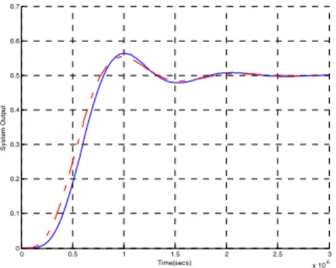
eigenvalues are -33.1963 and -944.3208. Using the same procedure that was performed above, the simulation of the full and reduced order models for a step input has generated the responses shown in Figure 15.

Figure 15. Input-to-output system step responses: full order model (solid line), transformed reduced order model (dashed line), and non-transformed reduced order model (dashed line).

0 0.5 1 1.5 2 2.5 3 -0.2

-0.1 0 0.1 0.2 0.3 0.4 0.5

Time[s]

S

y

s

tem

Out

p

ut

0 1 2 3 4 5 6 7

x 10-3 0

2 4 6 8 10 12 14

Time[s]

S

y

s

tem

O

ut

put

0 0.5 1 1.5 2 2.5 3

-0.005 0 0.005 0.01 0.015 0.02 0.025 0.03 0.035 0.04

Time[s]

S

y

s

tem

O

ut

p

ut

transformed reduced order model is more accurate than the response of the non-transformed reduced order model.

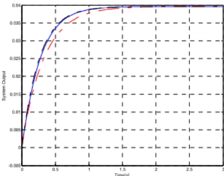
In a third example, different values of the capacitor, inductor, and resistor are considered such that the system eigenvalues are not very high (not very fast dynamics), but still one is larger than the other. Hence, the following values were considered {D = 0.4, R = 10.1 Ω, L = 3.305 H, C = 5.5 mF} and the eigenvalues are -3.901 and -14.099. For a step input, simulating the original and the transformed reduced order models along with the non-transformed reduced order model generated the results shown in Figure 16.

Figure 16. Input-to-output system step responses: full order model (solid line), transformed reduced order model (dashed line), and non-transformed reduced order model (dashed line).

As seen in Figure 16, the transformed reduced order model response is starting a little off from the original system response, however, it has a faster convergence than the non-transformed reduced order model response. The cause of this is due to the construction of the output matrix C = [0 1]; given:

( )

) ( ~

) ( ~

0 ) ( ~

) ( ~

t u B B t x

t x A A A

t x

t x

o r o

r o c r

o r

⎥ ⎦ ⎤ ⎢ ⎣ ⎡ + ⎥ ⎦ ⎤ ⎢ ⎣ ⎡ ⎥ ⎦ ⎤ ⎢

⎣ ⎡ = ⎥ ⎥ ⎦ ⎤ ⎢ ⎢ ⎣ ⎡

& &

[ ]

_⎥

⎦ ⎤ ⎢ ⎣ ⎡ =

) ( ~

) ( ~ 1 0 ) ( ~

t x

t x t

y

o r

where [Ar] is preset to the dominant eigenvalues (slow

dynamics), [Ao] is preset to the non-dominant eigenvalues

(fast dynamics), and [Ac] is the NN-estimated sub-matrix.

It is seen that ~y(t)=~xo(t), where~xo(t) is the solution of )

( ) ( ~ ) (

~ _{t A x t B u t}

x&_o = _{o o} + _o after setting it in the

formε~x&_o(t)=εA_o~x_o(t)+εB_ou(t) and letting ε~x&_o(t)=0

by using the singular perturbation technique. The sub-matrix [Ao] is set to have the fast dynamics (the -14.099

eigenvalue) regardless of the system response and is independent of the NN training. Hence, having ~y(t)

depending only on ~x_o(t), which was independent of the training (i.e., independent of [Ac]), makes the transformed

system response less accurate. However, if the output were to depend on ~x_r(t), which had the NN training (i.e., depends on [Ac]), such that C = [1 0], then the response

would be as shown in Figure 17, which is more accurate than the non-transformed reduced order model response.

Figure 17. Input-to-output system step responses: full order model (solid line), transformed reduced order model (dashed line), and non-transformed reduced order model (dashed line).

A fourth example that will produce complex eigenvalues and thus can not be reduced using the previously utilized singular perturbation technique is as follows: if the original system element values are set to

{D = 0.4, R = 18.6 Ω, L = 58 µH, C = 5.5 µF}, then the eigenvalues are found complex (-0.4888± j5.5776)×104. Here, since the system is a 2nd order and has complex eigenvalues, order model reduction can not be performed. 4.2 Control-to-Output System Model

The state space model of the control-to-output system is given by the system matrices:

A = _⎥

⎦ ⎤ ⎢

⎣ ⎡

− −

1/RC 1/C

1/L 0

, B = ⎥ ⎦ ⎤ ⎢ ⎣ ⎡

0

/L V_g

, C =

[

0 1

]

, E =

[ ]

0 . As seen in the above matrices, the system matrix [A] of the control-to-output state space model is the same as the input-to-output system. The only difference is that the input matrix [B] has changed to depend on the element

Vg instead of D. Thus, the eigenvalues will be the same

and the response will be of the same type as the input-to-output system. For instance, considering the elements of the system model given by {Vg = 15 V,R = 18.6 Ω, L =

58 mH, C = 5.5 µF}, the system output step response is

shown in Figure 18. As previously seen, the transformed reduced model response has a faster convergence than the response of the reduced model without system transformation.

or

B _∫

+ +

y(t)

u(t) ~x&r(t) ()

~ _t xr

K - r(t)

or

A

or C

+ +

+

or

E

0 0.5 1 1.5 2 2.5 3

-0.2 -0.1 0 0.1 0.2 0.3 0.4 0.5

Time[s]

S

y

s

tem

O

ut

put

Full order model Singularly perturbed reduced model Transformed reduced model Controlled reduced model

5. IMPLEMENTATION OF STATE FEEDBACK CONTROL ON THE REDUCED ORDER BUCK CONVERTER

Many control techniques such as H_∞control, robust control, stochastic control, intelligent control, etc. can be applied on the reduced order model to meet given design specifications. Yet, in this paper, since the Buck converter is a 2nd order system and is reduced to a 1st order, we will investigate system stability and enhancing performance by considering the simple pole placement method.

For the reduced order model in the system of Equations (38) and (39), a state feedback controller can be designed. For example, assuming that a controller is needed to provide the system with faster dynamical response, this can be done by replacing the system eigenvalues with new faster eigenvalues. Therefore: u(t)=−K~x_r(t)+r(t) (40) where K is to be designed based on the desired system eigenvalues. State feedback control for the transformed reduced order model is illustrated in Figure 19.

Figure 19. Block diagram of a state feedback control with {[A_or],[B_or],[C_or],[E_or]} overall reduced model matrices.

Replacing the control input u(t) in Equations (38) and (39) by the new control input in Equation (40) yields the following reduced system equations:

~x&_r(t)= A_or~x_r(t)+B_or[−K~x_r(t)+r(t)] (41) y(t)=C_or~x_r(t)+E_or[−K~x_r(t)+r(t)] (42) which can be re-written as:

~x&_r(t)= A_or~x_r(t)−B_orK~x_r(t)+B_orr(t) =[A_or−B_orK]x~_r(t)+B_orr(t)

y(t)=C_orx~_r(t)−E_orK~x_r(t)+E_orr(t) =[C_or−E_orK]~x_r(t)+E_orr(t) The closed-loop system model is:

~x&(t)= A_cl~x_r(t)+B_clr(t) (43) y(t)=C_cl~x_r(t)+E_clr(t) (44) such that the closed loop system matrix [Acl] will provide

the new desired system eigenvalues.

Example 3. Consider the input-to-output system presented in Section 4, where the eigenvalues are 3.901 and -14.099. Using the new transformation-based reduction technique, one obtains:

) ( ] 1212 . 0 [ ) ( ~ ] 3503 . 0 [ ) (

) ( ] 8051 . 5 [ ) ( ~ ] 901 . 3 [ ) ( ~

t u t

x t

y

t u t

x t

x

r r

r r

− + −

=

− + −

=

&

with the preserved eigenvalue of -3.901. Now, suppose that a new eigenvalue λ = -9, which will produce faster

system dynamics, is desired for this reduced order model. This objective can be achieved by first setting the desired characteristic equation as λ+9=0.

To determine the feedback control gain K, the characteristic equation of the closed-loop system is needed. This can be achieved using Equations (41) and (43) which yields:

(λI−A_cl)=0 → λI−[A_or −B_orK]=0

Knowing that A_or= -3.901 and B_or= -5.805, the closed-loop characteristic equation can be compared with the desired characteristic equation. Doing so, the feedback gain K is -0.8784. Hence, the closed-loop system now has the eigenvalue of -9. As stated previously, the objective of replacing eigenvalues is to enhance system performance. Simulating the reduced order model with the new eigenvalue for the same original system input (the step input) has generated the response shown in Figure 20.

Figure 20. Enhanced system step responses based on pole placement: full order model (solid line), transformed reduced order model (dashed line), non-transformed reduced order model (dashed line), and the controlled transformed reduced order (dashed line).

As shown in Figure 20, the new normalized system response is faster than the system response obtained without pole placement; the settling time in the reduced controlled system response is about 0.4 s while in the uncontrolled system response is about 1.3 s. This shows that even simple state feedback control using the transformation-based reduced order model can achieve the equivalent system performance enhancement obtained using complex and expensive control on the original full-order system.

6. CONCLUSION

A new method of control for the Buck converter is introduced in this paper. To achieve this control, the 2nd order Buck system was reduced to a 1st order system. This reduction was done by the implementation of a recurrent supervised NN to estimate certain elements [Ac] of the

transformed system matrix [A~ ], while the other elements [Ar] and [Ao] are set based on the system eigenvalues such

that [Ar] has the dominant eigenvalues (slow dynamics)

and [Ao] has the non-dominant eigenvalues (fast

to the state dynamics, based only on the system matrix [A]. After the transformed system matrix was obtained, the LMI optimization technique was used to determine the permutation matrix [P], which is required to obtain {[B~],[C~],[E~]}. The reduction process was then performed using the singular perturbation method, which operates on neglecting the faster-dynamics eigenvalues and using the dominant slow-dynamics eigenvalues to control the system. Simple state feedback control using pole placement was then applied on the reduced Buck model to obtain the desired Buck system response.

REFERENCES

[1] A. N. Al-Rabadi, An Approach to Exact Modeling of the PWM Switch, M.Sc. Thesis, ECE Dept., Portland State University (PSU), 1998.

[2] O. M.K. Alsmadi, Design of an Intelligent Neuro- Estimator for Complex Dynamic Systems, M.Sc. Thesis, ECE Dept., Tennessee State University (TSU), 1995. [3] P. Avitabile, J. C. O’Callahan, and J. Milani,

“Comparison of System Characteristics using Various Model Reduction Techniques,” 7th Int. Model Analysis Conf., Las Vegas, Nevada, February 1989.

[4] A. Bilbao-Guillerna, M. De La Sen, S. Alonso- Quesada, and A. Ibeas, “Artificial Intelligence Tools for Discrete Multiestimation Adaptive Control Scheme with Model Reduction Issues,” Proc. of the Int. Association of Science and Technology, Artificial Intelligence and Application, Innsbruck, Austria, 2004.

[5] S. Boyd, L. El Ghaoui, E. Feron, and V. Balakrishnan, Linear Matrix Inequalities in System and Control Theory, Society for Industrial and Applied Mathematics (SIAM), 1994.

[6] R. W. Erickson, Fundamentals of Power Electronics, Chapman and Hall, 1997.

[7] G. F. Franklin, J. D. Powell, and A. Emami-Naeini, Feedback Control of Dynamic Systems, 3rd _Edition,

Addison-Wesley, 1994.

[8] K. Gallivan, A. Vandendorpe, and P. Van Dooren, “Model Reduction of MIMO System via Tangential Interpolation,” SIAM J. of Matrix Analysis and Applications, Vol. 26, No. 2, pp. 328-349, 2004. [9] W. H. Hayt, J. E. Kemmerly, and S. M. Durbin, Engineering Circuit Analysis, McGraw Hill, 2007. [10] G. Hinton and R. Salakhutdinov, “Reducing the Dimensionality of Data with Neural Networks,” Science, pp. 504-507, 2006.

[11] R. Horn and C. Johnson, Matrix Analysis, Cambridge, 1985. [12] P. Kokotovic, R. O'Malley, and P. Sannuti, “Singular Perturbation and Order Reduction in Control Theory – An Overview,” Automatica, 12(2), pp. 123-132, 1976. [13] K. Ogata, Discrete-Time Control Systems, 2nd Edition, Prentice Hall, 1995.

[14] R. Skelton, M. Oliveira, and J. Han, Systems Modeling and Model Reduction, invited chapter in the Handbook of Smart Systems and Materials, Institute of Physics (IOP), 2004.

[15] A. N. Tikhonov, “On the Dependence of the Solution of Differential Equation on a Small Parameter,” Mat Sbornik (Moscow), pp. 193-204, 1948.

[16] R. J. Williams and Zipser, “A Learning Algorithm for Continually Running Full Recurrent Neural Networks,” Neural Computation, 1(2), pp. 270-280, 1989.