Analytical optimization of spread and change of exponential decay of generalized Wannier functions
in one dimension
Denis R. Nacbar1and Alexys Bruno-Alfonso2
1Programa de P´os-Graduac¸˜ao em Ciˆencia e Tecnologia de Materiais, Unesp, 17033-360 Bauru, S˜ao Paulo, Brazil 2Departamento de Matem´atica, Faculdade de Ciˆencias, Unesp, 17033-360 Bauru, S˜ao Paulo, Brazil
(Received 7 November 2011; revised manuscript received 22 March 2012; published 14 May 2012) Generalized Wannier functions of a couple of bands in a one-dimensional crystal are investigated. A lower bound for the global minimum of the total spread is obtained. Assumption of such a value being the minimum leads to a first-order differential equation for the transformation matrix. Simple analytical solutions leading to real generalized Wannier functions are presented for consecutive bands in a crystal with inversion symmetry. Results are displayed for a particle in a diatomic Kronig-Penney potential. For the lowest couple of bands, calculated single-band Wannier functions resemble orbitals of a diatomic molecule, whereas generalized Wannier functions seem like orthogonalized atomic orbitals. The latter functions are neither symmetric nor antisymmetric and display increased exponential decay. For the next two pairs of bands, Wannier functions retain their centers and symmetries, and exponential decay does not increase. Results are also shown to be in agreement with solutions of the eigenvalue problem of the band-projected position operator.
DOI:10.1103/PhysRevB.85.195127 PACS number(s): 71.20.−b, 71.15.Dx, 31.15.aq
I. INTRODUCTION
During the centennial year of Gregory Hugh Wannier, nearly a hundred publications have demonstrated that func-tions named after him are key computational tools in several research areas, such as insulators,1 magnetism,2,3 metals,4
photonics,5polymers,6semiconductors,7,8superconductivity,9 and electronic transport.10 Of course, applications have fueled basic research where Wannier functions (WFs) are the subject matter,11 and textbooks devote some attention to these functions.12–16 Since their introduction in 1937,17 the properties of WFs have challenged the solid-state physics community.18–20 This is mainly because of their lack of uniqueness, which is a feature inherited from Bloch functions (BFs). In fact, electronic BFs are common eigenfunctions of the Hamiltonian and translation operators that are conveniently chosen as periodic functions in the reciprocal space. Hence, taking normalization into account, the complex argument of BFs is determined up to a position-independent shift that should be periodic in the wave vector. Moreover, due to its periodicity, the Bloch function of each band may be represented by a Fourier series where coefficients are the Wannier functions of the band.
Contrasting the extended nature of BFs, Wannier functions are localized in real space and their nonuniqueness opens the possibility of optimizing the localization. The case of an electron in a one-dimensional (1D) crystal with inversion symmetry was investigated by Kohn in his outstanding paper of 1959.21He proved that the phase of the BFs may be chosen
in order to produce real, symmetric or antisymmetric, and exponentially localized WFs. The existence of an additional lo-calization in the form of a power law was demonstrated in 2001 by He and Vanderbilt.22This was extended in 2007 to deal with
maximally localized WFs of the noncentrosymmetric case.23
In the latter work, localization is measured by the variance, a criterion that was successfully used in 1997 by Marzari and Vanderbilt,24 to calculate WFs of three-dimensional crystals. Their approach leads with a generalization of WFs, in the sense established a few years after Kohn’s paper by Blount,25
des Cloizeaux,26 and Eilenberger,27 and became the basis of
modern computational packages, likeWANNIER90,28 devoted
to electronic-structure calculations. Moreover, the 1D version of those generalized functions has been investigated by using iterative and parallel-transport approaches.24,29
The aim of this work is to speed advances in the study of generalized Wannier functions (GWFs), by performing the analytical optimization of their total quadratic spread in the case of two consecutive bands of a 1D crystal with inversion symmetry. Several questions about the obtained GWFs are addressed, such as the possibility of being real, whether they may present increased exponential localization when compared with WFs of each band, how the inversion symmetry manifests on their shape, and what is their relation with atomic orbitals. In Sec.II, we review the construction of WFs and maximally localized GWFs. The problem is analytically solved in Sec.III, and numerical results and discussions for a diatomic Kronig-Penney model are given in Sec.IV. Final considerations are presented in Sec.V.
II. BASIC CONCEPTS AND EQUATIONS
Let us first recall basic ideas on Wannier functions of a 1D crystal. We denote a Bloch function of band indexj and wave numberkasψj,k(x). This family of functions satisfies the Schr¨odinger equation ˆH ψj,k(x)=Ej(k)ψj,k(x), the Bloch condition ψj,k(x+a)=eikaψj,k(x), where a is the lattice period, and the orthonormalization condition ψ∗
j,kψj′,k′ =
2π a−1δj,j′δ(k−k′), for any k and k′ in the first Brillouin
zone, where brackets refer to integration over the whole x
axis. Moreover, sinceψj,k+2π/a(x)=ψj,k(x), BFs are given by the Fourier series
ψj,k(x)=
n
wj,n(x)eikna, (1)
where the coefficientwj,n(x) is the Wannier function of the
wj(x)=ψj,k(x), where the line above the expression indicates the mean value over a Brillouin zone. We do not lose generality by assuming that Wannier functions of each band are real;23 i.e., BFs satisfy ψj,−k(x)=ψj,k∗ (x). More importantly, we suppose such WFs present maximal localization, i.e., minimal variance.24
To deal with Bloch functions of a group ofJ bands, we consider a rowJ-vectorkwhosejth component isψj,k. The orthonormalization of the BFs readsk†k′ =2π a−1δ(k−
k′)I. Moreover, we introduce the J-vector Wannier function
asW =k. Its normalization is written asW†W =I.
The centers of the WFs are the diagonal elements of the following matrix:
W†xW = x k†k′ =X(k), (2)
with
X(k)=i
a
0
u†ku˙kdx (3)
being the Berry connection.1 Hereu
k=exp(−ikx)k is the periodic part of k and a dot over a variable refers to differentiation with respect tok. More clearly, the center of
wj(x) is xj = W†xWj,j =Xj,j(k). It may be shown that
X(k) is Hermitian and satisfiesX(k+2π/a)=X(k).
To find the variance of WFs we define the matrix
W†x2W = x2k†k′ =Y(k), (4)
where
Y(k)=
a
0
˙
u†ku˙kdx (5)
is a Hermitian matrix satisfyingY(k+2π/a)=Y(k). Hence,
the variance ofwj(x) is given by
σj2= W†x2Wj,j−xj2=Yj,j(k)−(Xj,j(k))2. (6)
One may construct a set ofJ multiband Bloch functions ˜
ψj,k(x) by performing linear combinations of the J pure functions ψj,k(x). To do so, we introduce a J×J matrix
U(k) such that24
˜
ψj,k(x)= J
j′=1
ψj′,k(x)Uj′,j(k) (7)
applies forj =1, . . . ,J. These are also called quasi-Bloch functions, since they satisfy the Bloch condition but are not eigenfunctions of the Hamiltonian operator.
By introducing the row J-vector ˜k with j component ˜
ψj,k, we are able to rewrite Eq. (7) as ˜k =kU(k). Since ˜k†˜k′ =2π a−1δ(k−k′)U†(k)U(k), Bloch
func-tions remain orthonormalized provided U(k) is unitary, i.e., U†(k)U(k)=I. Moreover, the periodicity of ˜k ink, with
period 2π/a, leads toU(k+2π/a)=U(k). Therefore, GWFs
are given by W˜ =˜k and satisfy the orthonormalization conditionW˜†W˜ =I.
The center of thejth generalized Wannier function is ˜xj = W˜†xW˜
j,j =X˜j,j(k), where ˜
X(k)=U†(k)X(k)U(k)+iU†(k) ˙U(k) (8)
is a Hermitian matrix. Moreover, the variance of ˜wj(x) is given by
˜
σj2= W˜†x2W˜j,j −x˜j2=Y˜j,j(k)−(X˜j,j(k))2, (9)
where
˜
Y(k)=U†(k)Y(k)U(k)+U˙†(k) ˙U(k)
+i[U†(k)X(k) ˙U(k)−U˙†(k)X(k)U(k)]
=U†(k)[Y(k)−X2(k)]U(k)+X˜†(k) ˜X(k). (10)
To improve the quality of the generalized Wannier func-tions, we minimize their total quadratic spread, i.e, the sum of their variances,24which is given by
=
J
j=1
˜
σj2=Tr[ ˜Y(k)]−
J
j=1
˜
xj2. (11)
Since similar matrices have the same trace, this functional takes the form
=Tr[Y(k)−X2(k)
+X˜†(k) ˜X(k)]−
J
j=1
[ ˜Xj,j(k)]2
=0+2
J
j=1
j−1
j′=1
|X˜j,j′|2+
J
j=1
˜
X2
j,j−( ˜Xj,j)2, (12)
where0=Tr[Y−X2] does not depend onU. The second
and third terms in the second line of Eq.(12)are non-negative. Therefore,0is a lower bound for the total spread. Moreover,
if0is the minimum, then ˜X(k) should be a real and constant
diagonal matrix. According to Eq. (8), the optimization problem reduces to finding diagonal elements of ˜Xsuch that a
unitary transformation having the periodicity of the reciprocal lattice solves the first-order differential equation
˙
U(k)=i[X(k)U(k)−U(k) ˜X]. (13)
The resulting GWFs are real if the solution satisfies
U(−k)=U∗(k). (14)
We note that expressions in Eq.(12)resemble the previous approach in Ref.24, though we limit ourselves to the particular case of a 1D crystal. After some algebraic work, it is possible to prove that Eqs.(14),(19), and(20)in Ref.24correspond to the first, second, and third terms, respectively, in the second line of the present Eq.(12). In this latter version, however, only matrix elements of finite matricesY(k),X(k), and ˜X(k)
are involved, the invariance of the first term is more apparent, and the minimum variance is simply given in terms ofY(k)
and X(k). Moreover, for the case of a general 1D crystal,
it has been shown that eigenfunctions of the band-projected position operator are maximally localized GWFs.24Therefore,
diagonalization of that operator would lead to an optimal matrixU. Instead, in next section, such a matrix is obtained
III. EQUATIONS FOR TWO BANDS
Now we limit ourselves to the case of two bands, i.e.,J =2. Since U(k) is unitary, we have det[U(k)]=exp[i τ(k)],
where τ(k) is a real function. Moreover, we obtain
U1,2= −U2∗,1exp(iτ), U2,2=U1∗,1exp(iτ), and |det[U]| =
|U1,1|2+ |U2,1|2=1. Thus, there exist real functions θ(k),
φ1,1(k), and β(k), such that U1,1=cos(θ) exp(iφ1,1) and
U2,1=sin(θ) exp[i(φ1,1+β)]. Since |U2,2| = |U1,1|, we
conveniently denote the phase difference between U2,2 and
U1,1asα(k). Hence, matrixUmay be written as
U =eiτ2
cos(θ) −sin(θ)e−iβ
sin(θ)eiβ cos(θ)
e−iα 2 0
0 eiα2
. (15)
We assume that the WFs of each single band have been already optimized. Consequently,23 X1,1=x1andX2,2=x2.
Also, sinceXis Hermitian, diagonal terms are real, while
off-diagonal ones satisfy X1,2 =X∗2,1, with X2,1=C exp(i γ),
whereC(k) andγ(k) are real functions. Hence, assumingU(k)
leads to a global minimum0, we have ˜X1,1=x˜1, ˜X2,2=x˜2,
and ˜X1,2=X˜2,1=0. In this way, the sum of variances of the
maximally localized GWFs is
˜
σ12+σ˜22=0 =σ12+σ 2
2 −2C2. (16)
Moreover, Eq. (13) leads to a rather simple system of differential equations, namely,
˙
τ =(x1+x2)−( ˜x1+x˜2), (17)
˙
θ=Csin(β−γ), (18)
˙
α=x−x˜−2Ccos(β−γ) tan(θ), (19) and
˙
β =x+2Ccos(β−γ) cot(2θ), (20)
wherex =x2−x1and
x˜ =x˜2−x˜1
=x−2Ccos(β−γ) tan(θ)
− a
2π[α(π/a)−α(−π/a)]. (21)
The periodicity of U leads to conditions τ(k+
2π/a)=τ(k)+2π μτ, θ(k+2π/a)=(−1)μβθ(k)+π μθ, α(k+2π/a)=α(k)+2π μα, and β(k+2π/a)=β(k)+
π μβ, where μτ, μθ, μα, and μβ are integers, with μα−
μτ and μθ having the same parity. Moreover, Eq. (14) impliesτ(−k)= −τ(k)+2π ντ,θ(−k)=(−1)νβθ(k)+π νθ,
α(−k)= −α(k)+2π να, andβ(−k)= −β(k)+π νβ, where
ντ,νθ,να, andνβare integers, withνα−ντandνθhaving the same parity.
At this point we note that the expression in Eq. (15)for transformation matrixUhas the advantage of the differential
equation forτ(k) being decoupled. Solving Eq.(17)with the corresponding boundary conditions leads to τ(k)=aμτk+
π ντ, with μτ=[(x1+x2)−( ˜x1+x˜2)]/a. Then, by taking
μτ =0, the condition ˜x1+x˜2=x1+x2 holds; i.e., the sum
of centers of Wannier functions is conserved.24Additionally,
by choosingντ=0,τ(k) identically vanishes. In other words, the matrixU belongs to the special unitary groupSU(2). Of
course, in agreement with these choices,μα andμθ should have equal parities. The same thing applies toναandνθ.
Now we further restrict the discussion to the case of a 1D crystal with inversion symmetry and two consecutive bands labeled byj =1 andj =2. As shown in Appendix A, we may takeγ(k)=k x+sπ/2, wheres=0 (s=1) when the parities ofw1(x) andw2(x) are different (equal). Moreover,
C(k) is even (odd) whens=0 (s=1), andC(k) is periodic (antiperiodic) over the reciprocal lattice, whenn=2x/ais an even (odd) integer. At this point we note that Bloch functions at the edges of a band gap have different parities.30Therefore, the case s=1 and even n does not occur for consecutive bands.
Since ˙γ =x, Eqs.(18)–(20)may be rewritten as
˙
θ=Csin(ξ), (22)
˙
α=2Ccos(ξ) tan(θ)−2Ccos(ξ) tan(θ)+aμα, (23)
and
˙
ξ =2Ccos(ξ) cot(2θ), (24)
respectively, whereξ =β−γ. By combining Eqs.(22)and (24), it is easily shown that cos(ξ) sin(2θ)=A, whereAis a constant satisfying−1A1. In what follows, only cases
A= −1 andA=0 need to be considered.
On the one hand, A= −1 solves the problem pro-vided θ(k)= −π/4, ˙α=2(C−C)+aμα, ξ(k)=0 [i.e.,
β(k)=γ(k)],μθ =[(−1)n−1]/4, μβ =n=2x/a,νθ = [(−1)s
−1]/4, and νβ =s. Therefore, this solution applies fors=0 and evennonly, withμθ =νθ =νβ=0. Moreover, taking μα=να=0, with the same parity as μθ and νθ, Eq.(23)is solved to obtain
α(k)=2
k
0
[C(κ)−C]dκ, (25)
where C is the mean value of C(k). Furthermore, x˜ =
x+2Cleads to ˜x1=x1−Cand ˜x2=x2+C. The optimal
transformation matrix is
U= √1
2
1 e−inka/2
−einka/2 1
e−iα 2 0
0 eiα2
. (26)
On the other hand, A=0 solves the problem for odd values of n=2x/a, if ˙θ = −C, μθ =νθ=0, ˙α=a μα, andξ(k)= −π/2, i.e.,β(k)=γ(k)−π/2, withμβ =nand
νβ=s−1. Sinceμα andνα should be even, we takeμα =
να=0, which leads toα(k)=0 for everyk. Moreover,
θ(k)=
sπ/a
k
C(κ)dκ (27)
is odd (even) fors=0 (s=1), and the difference between centers is preserved, i.e.,x˜=x. Since the same happens with their sum, both centers remain untouched ( ˜x1=x1 and
˜
x2=x2). The transformation matrix becomes
U=
cos(θ) −i1−ssin(θ)e−inka/2
is−1 sin(θ)einka/2 cos(θ)
. (28)
for two consecutive bands, in the three symmetry cases of interest. This guarantees ˜reaches its global minimum, which is given by Eq.(16).
IV. NUMERICAL RESULTS AND DISCUSSION To be concrete, we deal with a diatomic version of the Kronig-Penney model,31,32 where a particle of mass m has potential energy given by
V(x)= −vh¯
2
m a
n
[δ(x−na+b/2)+δ(x−na−b/2)].
(29)
The indexnruns from−∞to+∞,v >0 is the dimensionless interaction strength, and b < a is an interatomic distance. The energy bands are obtained from E=h¯2ε/(2ma2) and
cos(ka)=μ(ε), where
μ(ε)=(1−v2/ε) cos(√ε)−2vsin(√ε)/√ε
+v2cos[(1−2b/a)√ε]/ε. (30) Since the potential presents inversion centers at integer multi-ples ofa/2, phases of Bloch functions are chosen appropriately in order to obtain maximally localized Wannier functions for each isolated band.30The numerical results below correspond
to parametersv=4 and b=3a/8. Moreover, energies and Bloch functions are calculated over a sample of 400 wave vectors uniformly spaced in the first Brillouin zone.
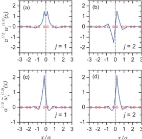
Figures 1(a)and 1(b) display the WFs of the lower two bands. Hence, the functions are labeled by superscript (1,2). It is apparent that single-band Wannier functions resemble molecular orbitals, with the first (second) band corresponding to the bonding (antibonding) one. Both molecular orbitals are centered at the origin of coordinates, i.e., x1=x2=0,
and the first (second) one is even (odd), corresponding to the cases=0 andn=0 in Sec.III. Moreover, the standard deviation of the WF for the first (second) band isσ1≈0.2579a
(σ2≈0.3323a). These functions decay exponentially with
coefficients that may be given in terms of the quantities
FIG. 1. (Color online) Wannier functions of (a) first and (b) second bands and (c,d) generalized Wannier functions for the pair (1,2) of bands. Open circles indicate atomic positions.
hj =a−1arccos[μ(εj)], whereεj is thejth root ofμ′(ε)=0. For parameters in the figure, we haveh1≈0.9969a−1 and
h2≈1.3542a−1. Hence,21 the decay of the WF of the first
(second) band is given byh1 (the minimum betweenh1 and
h2, i.e., h1). This corresponds to the distance from the real
k axis to the closest branch points of εj(k). Of course, an additional power-law decay with exponent 3/4 also occurs.22
Generalized Wannier functions for the lower two bands are calculated by the transformation matrix in Eq.(26). Since
n=0, it takes a simpler form, namely,
U(k)= √1
2
e−iα2(k) e iα(k)
2
−e−iα2(k) e iα(k)
2
, (31)
whereα(k), given by Eq.(25), is an odd function. Figures1(c) and1(d)display results for the same parameters as Figs.1(a) and1(b). The centers of these functions are ˜x1≈ −0.21125a
and ˜x2≈0.21125a. Moreover, they present identical standard
deviations, namely ˜σ1=σ˜2≈0.1516a. This means that the
total variance has decreased by about 74%. It is worth noting that these GWFs are neither symmetric nor antisymmetric. Indeed, crystal symmetry manifests in the sense that they are mirror images of each other about linex =0, i.e., ˜w(12,2)(x)=
˜
w(11,2)(−x). As shown in AppendixB, this follows from choices leading to Eq.(31)and gauge choices21ψ
1,k(−x)=ψ1,−k(x) andψ2,k(−x)= −ψ2,−k(x). We also note that, because of the
diagonal character of ˜X(k), the conditionw˜(1,2)
1 |x|w˜ (1,2) 2 =0
should apply. The symmetry relation between the GWFs also leads to this result, namely,
˜
w1(1,2)x w˜(12,2)=
∞
−∞
xw˜(11,2)(x) ˜w2(1,2)(x)dx
=
∞
−∞
xw˜(11,2)(x) ˜w1(1,2)(−x)dx=0, (32)
since ˜w(11,2)(x) ˜w1(1,2)(−x) is an even function.
Regarding the asymptotic behavior of GWFs, symmetry allows us to focus on ˜w(11,2)(x) only. We notice that both the coefficient of exponential decay and the exponent of the power-law decay may be extracted from the list of probabilities for the particle to be found within each unit cell.22,23 For the functions in the figure, we have obtained
identical parameters forx → −∞andx→ ∞. Namely, the coefficient of exponential localization is noticeably larger for these generalized WFs than for functions in Figs.1(a)and1(b), and it is found to beh2≈1.3542. This is due to cancellation
between terms in the linear combination ofψ1,k andψ2,k at their common branch points, while farther branch points of
ψ2,k survive. The 3/4 power-law decay also occurs.
When a minimization procedure of total variance is applied to the pair (2,3) of bands, the results are quite different. This is because the symmetries of WFs of second and third bands are different, while the distance between their centers is an odd multiple of half period. In fact, it is apparent in Figs.2(a)and2(b)thatx1 =0 andx2 =a/2. Moreover, the
variance and coefficient of exponential localization for the second (third) band are σ1≈0.3323a and h1=0.9968a−1
(σ2≈0.3468a andh3=0.7994a−1), respectively. This case
FIG. 2. (Color online) Wannier functions of (a) second and (b) third bands and (c,d) generalized Wannier functions for the pair (2,3) of bands. Open circles indicate atomic positions.
the generalized functions shown in Figs. 2(c) and 2(d). By comparing WFs and GWFs, we observe that the centers and symmetries are preserved, while the total spread diminishes. On the one hand, the properties ˜w(21,3)(−x)= −w˜1(2,3)(x) and
˜
w2(2,3)(a−x)=w˜(22,3)(x) are shown in AppendixBto follow from Eq.(28)and gauge choices21ψ
2,k(−x)= −ψ2,−k(x) and ψ3,k(a−x)=ψ3,−k(x). On the other hand, the variances of w(21,3)(x) and w(22,3)(x) are ˜σ1 ≈0.3157a and ˜σ2 ≈0.2108a,
respectively, corresponding to a decrease in total variance of about 37%. Furthermore, both GWFs decay exponentially with the same coefficient, namely,h3=0.7994a−1. To understand
this, it may be noticed that the first, second, and third gaps with coefficientsh1,h2, andh3are relevant for the pair (2,3)
of bands. Therefore, even if cancellation at branch points of the second gap were to occur, min(h1,h3)=h3 would dominate
the decay.
The results are similar for the pair (3,4) of bands. As shown in Figs. 3(a) and 3(b), now single-band WFs have
FIG. 3. (Color online) Wannier functions of (a) third and (b) fourth bands and (c,d) generalized Wannier functions for the pair (3,4) of bands. Open circles indicate atomic positions.
the same parity but their centers are separated by half a period. Therefore, the transformation in Eq. (28) leads to the maximally localized GWFs displayed in Figs. 3(c) and 3(d). Clearly, centers and symmetries are preserved again. Namely, the conditions ˜w1(3,4)(a−x)=w˜1(3,4)(x) and
˜
w(32,4)(−x)=w˜(32,4)(x) hold. These properties may be derived from Eq.(28)and gauge choices21ψ3,k(a−x)=ψ3,−k(x) and ψ4,k(−x)=ψ4,−k(x) (see Appendix B). Moreover, standard deviations of WFs (σ1=0.3468a,σ2=1.1982a) and GWFs
( ˜σ1=0.6915a, ˜σ2=0.9618a), corresponding to a decrease in
total spread of about 10%. It is interesting to note in Fig.3that one function has become broader [Fig.3(a)→Fig.3(c)] while the other has narrowed [Fig. 3(b)→Fig. 3(d)]. At the same time, the first one has slowed down its exponential decrease. In fact, the coefficient of decay of both GWFs is found to be
h4≈0.0545a−1.
For the sake of completeness, we now compare the results presented above with those obtained by diagonalization of the position operator x. Conveniently, this operator can be represented in terms of Wannier functionswj,n(x), withj =
1, . . . ,J andnrunning over the integers. The matrix elements ofxin this basis are given by
x(j,n),(j′,n′) = wj,n|x|wj′,n′ =Xj,j′,n′−n+na δj,j′δn,n′,
(33)
with
Xj,j′,n =exp(−inak)Xj,j′(k) (34)
being the nth Fourier coefficient of Xj,j′(k). Clearly, the
matrix is Hermitian, and its eigenvalues are the centers of GWFs with maximal localization.24 It is worth noting
that the spectrum of x is periodic, with period a, and the corresponding eigenvectors are the coordinates of GWFs in the basis set of single-band WFs. Therefore, it suffices to accurately determine those eigenvalues between −a/2 and a/2. With this in mind, approximate eigenvalues may be calculated by truncating the basis, namely, by taking
n= −N,1−N, . . . ,−1,0,1, . . . ,N, for a sufficiently large integerN. The truncated matrix is of dimensionJ(2N+1)×
J(2N+1), and accuracy may be improved by increasing the value of N. This is apparent in Fig. 4, where the two relevant eigenvalues for the pair (1,2) of bands are shown as a function ofN. In fact, the lower [upper] eigenvalue in Fig.4(a)
[Fig.4(b)] rapidly converges to the center of ˜w1(x) [ ˜w2(x)]
as N increases. It should also be remarked that eigenvalues forN=0 coincide with the corresponding limit values. This is in agreement with the analytical development in Sec. II, where ˜x1and ˜x2 have been shown to bex1−C andx2+C,
respectively, withx1=x2 =0 andC=x(1,0),(2,0)=x(2,0),(1,0).
We have also checked the convergence to GWFs of linear combinations of the J(2N+1) WFs, with the coefficients being the corresponding eigenvectors. For the considered parameters of the 1D crystal, the scalar product between the analytically obtained GWFs and the linear combinations is above 0.99, for all values ofN. And, apparently, convergence to 1 is quite rapid. Nevertheless, good agreement between the exponentially decaying tails may require large values of N. A similar analysis may be done for other pairs of bands.
V. CONCLUSIONS
The total variance of generalized Wannier functions of two consecutive bands in a 1D crystal with inversion symmetry has been minimized by following a straightforward analytical approach. This has led to real generalized Wannier functions of maximal localization. Different expressions have been given for the cases where the distance between the centers of single-band Wannier functions is either an even or an odd multiple of half a period of the crystal. Numerical results were presented for the lowest four bands of a particle subject to a diatomic Kronig-Penney potential. For the lowest couple of bands, calculated single-band (generalized) Wannier functions resemble molecular (orthogonalized atomic) orbitals, and the latter display increased exponential localization. Moreover, the centers change and the generalized functions are neither symmetric nor antisymmetric, but they are related by an inversion-symmetry transformation. Instead, for the second and third pairs of consecutive bands, Wannier functions con-serve both center and inversion symmetry, while exponential decay does not increase. Changes in the coefficient of such decay have been explained in terms of branch points of Bloch functions of each band.
The presented explicit expressions of the matrix that transforms the Bloch function into quasi-Bloch functions noticeably simplify computation of generalized Wannier functions, making them available to a broader community. Moreover, convergence of truncation and iterative procedures may be further tested. This has been done for the eigenvalue problem of the band-projected position operator. At the same time, interesting properties of symmetry and decay have been explained. Calculated functions should find applications in the study of defect-induced localized states with energy lying within the gap separating the considered pair of bands, but future work should deal with generalized Wannier functions of several bands. We expect similar efforts will be devoted to one-dimensional crystals lacking inversion symmetry, as well as two- and three-dimensional crystals.
ACKNOWLEDGMENTS
We thank the Brazilian Agencies CNPq and FAPESP for financial support.
APPENDIX A: OFF-DIAGONAL TERMX2
,1(
k)
In this section, properties of real functionsC(k) andγ(k) satisfyingX2,1(k)=C(k) exp[i γ(k)] are demonstrated. From
Eq.(3), we have
X2,1(k)=i
a
0
u∗2,k(x) ˙u1,k(x)dx
=
a
0
ψ2∗,k(x)[iψ˙1,k(x)+x ψ1,k(x)]dx. (A1)
Ifwj(x) obeyswj(x)=sjwj(2xj −x), then it is even (odd) about x =xj, when sj =1 (sj = −1). The correspond-ing Bloch function satisfies ψj,k(x)=sjψj,−k(2xj −x)=
sjψj,k∗ (2xj −x). Taking the Bloch condition and orthogonal-ity of Bloch functions into account, we obtain
X2,1(k)=s1s2
2x1
2x1−a
ψ2,k(2x2−x)[iψ˙1∗,k(2x1−x)
+x ψ1∗,k(2x1−x)]dx
=s1s2e2ik x
a
0
ψ2,k(x)[iψ˙1∗,k(x)
+(2x1−x)ψ1∗,k(x)]dx
= −s1s2e2ik xX∗2,1(k). (A2)
Therefore, we may write
e−ik xX2,1(k)=(−1)s[e−ik xX2,1(k)]∗, (A3)
where (−1)s= −s1s2, and we take s=0 (s=1) when the
parities ofw1(x) and w2(x) are different (coincide). In the
first (second) case, e−ik xX
2,1(k) is real [pure imaginary]
and may be written as C(k) [i C(k)]. These results may be summarized asX2,1(k)=C(k) exp[i γ(k)], whereC(k) is real
andγ(k)=k x+s π/2.
From Eq.(A1)we may derive inversion-symmetry prop-erties ofC(k). In fact, since X2,1(−k)=X∗2,1(k), we obtain
C(−k)=(−1)sC(k). This meansC(k) is even (odd) fors
=0
(s=1). Furthermore, sinceX2,1(k) has the periodicity of the
reciprocal lattice, C(k) satisfiesC(k+2π/a)=(−1)nC(k), withn=2x/a; i.e., it is periodic (antiperiodic) whennis even (odd).
APPENDIX B: SYMMETRY AND GENERALIZED WANNIER FUNCTIONS
To obtain a symmetry relation between the generalized Wannier functions of a couple of bands having Wannier func-tions centered atx=0 with the first (second) one being an even (odd) function, we take into account conditionsψ1,k(−x)=
ψ1,−k(x) andψ2,k(−x)= −ψ2,−k(x). From Eq.(31), we have
˜
ψ1(1,k,2)(x)= e
−i α2(k) √
2 [ψ1,k(x)−ψ2,k(x)] (B1)
and
˜
ψ2(1,k,2)(x)= e i α(k)
2 √
Moreover, according to Eq.(25),α(k) is an odd function, and we obtain
˜
ψ2(1,k,2)(x)= e
−i α(−k) 2 √
2 [ψ1,−k(−x)−ψ2,−k(−x)]= ˜
ψ1(1,−,2)k(−x).
(B3)
Taking the average over the first Brillouin zone, this leads to ˜
w2(1,2)(x)=w˜1(1,2)(−x).
Now, let us try to demonstrate that centers and symmetries of ˜w1(x) and ˜w2(x) coincide with those ofw1(x) andw2(x),
respectively, whenn=2x/ais odd. To be concrete, we con-sider the pair (2,3) in Sec.IV, whereψ2,k(−x)= −ψ2,−k(x)
and ψ3,k(a−x)=ψ3,−k(x). We note that s=0 (opposite
symmetries), θ(k) is odd, and n=1. Then, from Eq. (28), we have
˜
ψ1(2,k,3)(x)=cos(θ(k))ψ2,k(x)−i e ika
2 sin(θ(k))ψ3,k(x) (B4)
and
˜
ψ2(2,k,3)(x)= −i e−ika2 sin(θ(k))ψ2,k(x)+cos(θ(k))ψ3,k(x).
(B5)
According to the Bloch condition, this leads to
˜
ψ1(2,k,3)(−x)= −cos(−θ(−k))ψ2,−k(x)
−i e−ika2 sin(−θ(−k))ψ3,
−k(x)
= −cos(θ(−k))ψ2,−k(x)
+i e−ika2 sin(θ(−k))ψ3,
−k(x)
= −ψ˜1(2,−,3)k(x) (B6)
and ˜
ψ2(2,k,3)(a−x)=i eika2 sin(−θ(−k))ψ2,
−k(x)
+cos(−θ(−k))ψ3,−k(x)
= −i eika2 sin(θ(−k))ψ2,
−k(x)
+cos(θ(−k))ψ3,−k(x)
=ψ˜2(2,−,3)k(x). (B7)
Hence, after averaging over the first Brillouin zone, the results are ˜w(21,3)(−x)= −w˜1(2,3)(x) and ˜w(22,3)(a−x)=w˜2(2,3)(x).
The conservation of symmetry for pair (3,4) in Sec.IVmay be proved in the same way. In doing so, the conditionsψ3,k(a−
x)=ψ3,−k(x) andψ4,k(−x)=ψ4,−k(x) should be taken into account. Moreover, we note thats=1 (same symmetry),θ(k) is even, andn= −1.
1R. Resta,Eur. Phys. J. B79, 121 (2011).
2E. Kr¨uger and H. Strunk, J. Supercond. Novel Mag. 24, 2103 (2011).
3T. Berlijn, D. Volja, and W. Ku,Phys. Rev. Lett.106, 077005 (2011). 4T. Bazhirov, J. Noffsinger, and M. L. Cohen,Phys. Rev. B 84,
125122 (2011).
5T. Stollenwerk, R. Frank, A. Lubatsch, O. Zaitsev, S. Zhukovsky, D. Chigrin, and J. Kroha,Appl. Phys. B105, 163 (2011).
6M. Lorenz, D. Usvyat, and M. Sch¨utz,J. Chem. Phys.134, 094101 (2011).
7D. Benson, O. F. Sankey, and U. H¨aussermann,Phys. Rev. B84, 125211 (2011).
8J. S. Lee, G. A. H. Schober, M. S. Bahramy, H. Murakawa, Y. Onose, R. Arita, N. Nagaosa, and Y. Tokura,Phys. Rev. Lett. 107, 117401 (2011).
9M. Casula, M. Calandra, G. Profeta, and F. Mauri,Phys. Rev. Lett. 107, 137006 (2011).
10M. Shelley, N. Poilvert, A. A. Mostofi, and N. Marzari,Comput. Phys. Commun.182, 2174 (2011).
11M. Chen, G.-C. Guo, and L. He,J. Phys.: Condens. Matter 23, 325501 (2011).
12N. W. Ashcroft and N. D. Mermin,Solid State Physics(Brooks Cole, Belmont, 1976).
13O. Madelung,Introduction to Solid-State Physics(Springer, Berlin, 1978).
14R. M. Martin,Basic Electronic Structure(Cambridge University Press, Cambridge, 2004).
15Conceptual Foundations of Materials, edited by S. G. Louie and M. L. Cohen (Elsevier, Amsterdam, 2006).
16Condensed Matter Physics, 2nd ed., edited by M. P. Marder (Wiley, Hoboken, 2010).
17G. H. Wannier,Phys. Rev.52, 191 (1937). 18G. Nenciu,Commun. Math. Phys.91, 81 (1983).
19C. Brouder, G. Panati, M. Calandra, C. Mourougane, and N. Marzari,Phys. Rev. Lett.98, 046402 (2007).
20H. D. Cornean, A. Nenciu, and G. Nenciu,J. Phys. A41, 125202 (2008).
21W. Kohn,Phys. Rev.115, 809 (1959).
22L. He and D. Vanderbilt,Phys. Rev. Lett.86, 5341 (2001). 23A. Bruno-Alfonso and D. R. Nacbar, Phys. Rev. B75, 115428
(2007).
24N. Marzari and D. Vanderbilt,Phys. Rev. B56, 12847 (1997). 25E. I. Blount,Solid State Phys.13, 305 (1962).
26J. D. Cloizeaux,Phys. Rev.135, A685 (1964); 135, A698 (1964). 27G. Eilenberger, Z. Phys. A180, 43 (1964).
28A. A. Mostofi, J. R. Yates, Y.-S. Lee, I. Souza, D. Vanderbilt, and N. Marzari,Comput. Phys. Commun.178, 685 (2008).
29J. Bhattacharjee and U. V. Waghmare,Phys. Rev. B 71, 045106 (2005).
30A. Bruno-Alfonso and G.-Q. Hai,J. Phys.: Condens. Matter15, 6701 (2003).
31F. B. Pedersen, G. T. Einevoll, and P. C. Hemmer,Phys. Rev. B44, 5470 (1991).