Comment on "Biotic pump of atmospheric moisture as driver of the hydrological cycle on land" by A. M. Makarieva and V. G. Gorshkov, Hydrol. Earth Syst. Sci., 11, 1013–1033, 2007

(1)

HESSD

6, 401–416, 2009

Commentary on Makarieva and

Gorshkov

A. G. C. A. Meesters et al.

Title Page

Abstract Introduction

Conclusions References

Tables Figures

◭ ◮

Back Close

Full Screen / Esc

Printer-friendly Version

Interactive Discussion Hydrol. Earth Syst. Sci. Discuss., 6, 401–416, 2009

www.hydrol-earth-syst-sci-discuss.net/6/401/2009/ © Author(s) 2009. This work is distributed under the Creative Commons Attribution 3.0 License.

Hydrology and Earth System Sciences Discussions

Papers published inHydrology and Earth System Sciences Discussionsare under open-access review for the journalHydrology and Earth System Sciences

Comment on “Biotic pump of atmospheric

moisture as driver of the hydrological

cycle on land” by A. M. Makarieva and

V. G. Gorshkov, Hydrol. Earth Syst. Sci.,

11, 1013–1033, 2007

A. G. C. A. Meesters, A. J. Dolman, and L. A. Bruijnzeel

Faculty of Earth and Life Sciences, VU University, Amsterdam, The Netherlands

Received: 19 November 2008 – Accepted: 20 November 2008 – Published: 16 January 2009

Correspondence to: A. G. C. A. Meesters ([email protected])

(2)

HESSD

6, 401–416, 2009

Gorshkov

Title Page

Tables Figures

◭ ◮

Back Close

Full Screen / Esc

Interactive Discussion Abstract

In their paper “Biotic pump of atmospheric moisture as driver of the hydrological cycle on land”, Makarieva and Gorshkov (Hydrol. Earth Syst. Sci., 11, 1013–1033, 2007) de-rive from “previously unstudied” properties of atmospheric water vapor, the existence of a hitherto unknown “evaporative force”. From this, a novel physical principle is

de-5

duced, according to which low-level air flows from regions with weak, to regions with strong evaporation. As such, natural forests are claimed to “suck in” moist air from the ocean, a process labeled the “biotic pump of atmospheric moisture”.

This commentary focuses on the physical foundations of the biotic pump theory, which is presented as revolutionary by Makarieva and Gorshkov. It is shown that the

10

“evaporative force” on which the theory is built, is an untenable result of confused and inappropriately used physical principles. The problem of moisture transport and its dependence on vegetation cover considered by Makarieva and Gorshkov is certainly important, but cannot be solved along the lines proposed by them.

1 Introduction

15

How moisture is transported from oceans to land, and the precise role of vegetation in this process, constitute key questions in our understanding of the hydrological cycle. Early modeling studies have indicated that the complete conversion of the Amazonian rain forest to pasture would lead to increased surface temperatures, a reduction in pre-cipitation, and reduced atmospheric moisture convergence (e.g. Nobre et al., 1991;

20

Henderson-Sellers et al., 1993). Subsequent modeling work has by and large con-firmed these results, although the magnitude of the predicted effects seems to have diminished as models became more and more sophisticated (Bruijnzeel, 2004; Costa, 2004). In addition, several modeling studies have even suggested the existence of tele-connection patterns between (Amazonian) deforestation and changes in

precipi-25

tation in remote areas (e.g. Gedney and Valdes, 2000; Werth and Avissar, 2002). In

(3)

HESSD

6, 401–416, 2009

Gorshkov

Title Page

Tables Figures

◭ ◮

Back Close

Full Screen / Esc

Interactive Discussion most of these studies, decreased atmospheric moisture availability due to reduced soil

water uptake and rainfall interception after forest removal, is considered a key underly-ing cause of such model predictions. At the large scale, this interacts with decreased moisture convergence through reduced aerodynamic surface roughness whereas at sub-regional scales, cause and e_ffect are complicated by meso-scale circulations (Silva

5

Dias et al., 2002; Moore et al., 2007), subtleties in the precise triggering of convection, the generation of squall lines (idem), and effects of local topography (Dolman et al., 1999; Roy and Avissar, 2002).

Recently, a new theory has been advanced that claims a new role for forest in the generation of rainfall (Makarieva and Gorshkov, 2007; referred to in the following as

10

M&G). In fact, the paper by M&G has an even wider scope in that it aims to explain the causative mechanisms underlying the entire global circulation (M&G’s Sect. 3.3). Knowledge from a broad range of disciplines is combined into a coherent picture, which makes the new theory no doubt attractive to many readers and organizations interested in forest conservation or assessing the impact of land-cover change on hydrology and

15

rainfall. However, upon closer scrutiny, it would appear that some fundamental points have been neglected by M&G, whereas, in addition, the paper raises a number of is-sues that warrant further discussion. The basic question addressed by M&G is: how is the land kept moistened? This question is answered by relating the theory of mois-ture transport and spatial distribution of precipitation to the presence or absence of

20

(large tracts of) forest. M&G invoke “previously unstudied” properties of atmospheric water vapor, which can be either in or out of aerostatic equilibrium (M&G, Sect. 3.1). From this, they derive a hitherto unknown “evaporative force” (M&G, Sect. 3.2). A novel physical principle is then formulated, according to which low-level air moves from areas with weak evaporation to areas with more intensive evaporation. Next, natural forests

25

are claimed to “suck in” moist air from the ocean, a process labeled the “biotic pump of atmospheric moisture”. This principle constitutes the core of their paper.

(4)

HESSD

6, 401–416, 2009

Gorshkov

Title Page

Tables Figures

◭ ◮

Back Close

Full Screen / Esc

Interactive Discussion the disequilibrium on which their theory is based does exist, its effect on the transport

of water vapor will be shown to be negligible, in contradiction to the results derived by M&G. In summary, M&G’s concept of “evaporative force” will be shown to be simply untenable.

2 Two kinds of equilibrium

5

2.1 “Traditional” theory of equilibrium

There are two kinds of equilibrium to be distinguished, and it is critically important not to confuse the two. The first, which we shall call “bulk-equilibrium” for convenience sake, is the well-known hydrostatic equilibrium, i.e. the pressure difference over a vertical column of air equals the weight per area of the column (e.g. Landau and Lifshitz, 1987)

10

−

∂p

∂z =ρg (1)

wherez=height,p=pressure,ρ=mass density andg=acceleration due to gravity. This equation is fundamental in meteorology in that deviations from equilibrium cause a ver-tical motion according to the verver-tical Euler equation:

ρd w d t =−

∂p

∂z −ρg (2)

15

(wherew=vertical velocity, positive when upward; andt=time) which will continue until equilibrium is restored.

Equations (1) and (2) are mechanical equations which apply to air as such (not its separate components), and they determine the motion of air parcels as a whole. For a homogeneous mixture, hydrostatic equilibrium corresponds to a density profile which

20

can be derived by combining Eq. (1) with the equation-of-state:

p=ρ(R/M)T (3)

(5)

HESSD

6, 401–416, 2009

Gorshkov

Title Page

Tables Figures

◭ ◮

Back Close

Full Screen / Esc

Interactive Discussion (whereR=universal gas constant per mol,M=mean mass per mol of the mixture, and

T=absolute temperature). Assuming T to be constant for convenience, this leads to a height distribution:

ρ(z)=ρ_surexp(−z/h) (4)

in whichhis the scale height for the mixture:

5

h= RT

Mg (5)

Upon substituting M=29 g mol−1 _{(the value for dry air) and} _T

=288 K one obtains h=8.4 km.

Air consists of components which may be indicated with the subscripti. The mass densityρ is then the sum of the densities of the componentsi. Further, Dalton’s law

10

states that the pressurepis the sum of the partial pressuresp_i of the components, for which the equation-of-state is:

pi =ρi(R/Mi)T (6)

The second kind of equilibrium is thermodynamic equilibrium. We will call this “component-equilibrium” for convenience, since it applies to each component of the

15

mixture separately. According to Boltzmann’s equation, ifT is constant the thermody-namic equilibrium density of thei-th component is given by:

ρi(z)=ρi ,surexp

−

E_i(z) RT

(7)

in whichE_i(z)=M_igz or the potential energy per mol due to gravitation (Landau and Lifshitz, 1987, paragraph 59). This distribution can also be written as:

20

(6)

HESSD

6, 401–416, 2009

Gorshkov

Title Page

Tables Figures

◭ ◮

Back Close

Full Screen / Esc

Interactive Discussion in which the scaling heighth_i is given by:

h_i = RT

Mig

(9)

with Mi the molar mass of thei-th constituent. Equations (8) and (9) are similar to Eqs. (4) and (5), but now every component has its own scaling height. For water vapor atT=288 K, hi=13.5 km, which is much larger than that for nitrogen or oxygen:

5

viz. 8.7 km and 7.6 km, respectively. Using the equation-of-state per component (6), the component equilibrium profile can be shown to satisfy the counterpart of Eq. (1):

−

∂p_i

∂z =ρig (10)

However, this component-equilibrium should not be called “hydrostatic” or “aerostatic” equilibrium, and is not to be thought of in mechanical terms (such as partial pressures

10

being in balance with the weights of the respective components), as is sometimes done by M&G (e.g. in the beginning of their Sect. 3.1). It must be emphasized that the component-equations (8, 9, and 10) are valid only for thermodynamic equilibrium.

Whilst bulk-equilibrium is restored by macroscopic motion, restoring of (thermody-namic) component-equilibrium requires a process in which the components move

sep-15

arately. The only process capable of this is (molecular) diffusion (Landau and Lifshitz, 1987, Sect. 57). However, this is a very slow process, compared with macroscopic atmospheric transport mechanisms as molecular diffusion coefficients in the lower tro-posphere are in the order of ca. 10−5_m2_s−1_{(Tennekes and Lumley, 1990). The relation} between molecular diffusion and large-scale thermodynamic equilibrium under an

ex-20

ternal force, first elucidated by Einstein, has been described by Van Kampen (1983), Dill and Bromberg (2003), and (very briefly) by Landau and Lifshitz (1987), Sect. 59. The result is that the equilibrium-restoring diffusive fluxF_i (positive when upward) can be expressed in the language of M&G as:

F_i =−νi

_∂ρ

i ∂z +

ρi h_i

(11)

25

(7)

HESSD

6, 401–416, 2009

Gorshkov

Title Page

Tables Figures

◭ ◮

Back Close

Full Screen / Esc

Interactive Discussion whereν_i is the molecular diffusivity. The first term represents the common Fick’s Law,

whereas the second term is a modification due to the acting of gravity on the molecules. What then are the practical consequences of these two equilibria? These are very different for (hydrostatic) bulk-equilibrium on the one hand, and (thermodynamic) component-equilibrium on the other. Deviations from bulk-equilibrium cause

macro-5

scopic motions which act to restore equilibrium in a highly efficient manner. It is well known (Wallace and Hobbs, 1977; Holton, 1979; Dutton, 1986; and many others) that air is usually in hydrostatic equilibrium, to very good approximation, except when lo-cal phenomena such as up- and down-drafts occur. On the other hand, deviations of component-equilibrium cannot cause restoring motions, only diffusive fluxes which are

10

very weak (Eq. 11). Because component-disequilibrium has so little e_ffect, it is barely considered in atmospheric science as a causative factor, except in relation to interface-processes which always act on the micro-scale (e.g. evaporation at a surface, cloud microphysics).

2.2 The approach of M&G to the two kinds of equilibrium

15

The key question in the context of the “evaporative force” postulated by M&G is whether component-equilibrium is of importance to macroscopic transport in the atmosphere. M&G deny this correctly for water vapor, their argument being (summarized) that vapor is continuously entering the atmosphere at the surface by evaporation, whereas it is removed at greater altitudes by condensation and precipitation. Hence, observed vapor

20

profiles are much more compressed than the equilibrium-profile predicted by Eq. (8) using hi=13.5 km at T=288 K. Qualitatively speaking, this is correct. However, for dry air, there is a complication. Dry air consists of several components, each with a different molar mass and consequently with different scaling heights. M&G accept the fact that these components are well-mixed in the troposphere (McEwan and Phillips,

25

1975; Wallace and Hobbs, 1977, and thus that dry air has a near-constant composition. Hence, it can be treated as a single component, with a molar mass ofMd=29 g mol−

1

(8)

HESSD

6, 401–416, 2009

Gorshkov

Title Page

Tables Figures

◭ ◮

Back Close

Full Screen / Esc

Interactive Discussion Next, M&G make a very important assumption, stating that for the dry air (d)

com-ponent, component-equilibrium should always hold:

−

∂p_d

∂z −ρdg=0 (12)

It should be noted first of all that this assumption is in sharp contradiction to the “tradi-tional” assumption that it is the bulk-equilibrium rather than the component-equilibrium

5

that is maintained. The reason is that bulk-equilibrium is linked to dry air (d) equilibrium and vapor (v) equilibrium by:

−

∂p

∂z −ρg=

−

∂p_d

∂z −ρdg

+

−

∂pv ∂z −ρvg

(13)

Since it is taken for granted that the vapor component is not in equilibrium, acceptance of Eq. (12) implies that there is no bulk-equilibrium either. This consequence is already

10

announced in M&G’s Sect. 3.1 (“Moist air does not conform to either Eq. (7) or Eq. (8)”), and is applied in M&G’s Sect. 3.2 after M&G’s Eq. (10). It constitutes a key building block in the derivation of M&G’s concept of “evaporative force”.

It is unclear why M&G have replaced the “traditional” assumption of bulk-equilibrium (Eq. 1) with an assumption of component-equilibrium for dry air (Eq. 12). The

attri-15

bution of M&G’s Eq. (7) to Landau and Lifshitz (1987) appears inappropriate. One consideration is that, unlike for water vapor, the equilibrium is not affected by inflow and outflow of the component. Also, we have already noted that M&G speak in a con-fused way about component-equilibrium as “hydrostatic equilibrium”. Furthermore, the following citation from M&G seems key in this respect:

20

“In agreement with Dalton’s law, partial pressures of different gases in a mixture inde-pendently come in or out of the equilibrium. The non-equilibrium state of atmospheric water vapor cannot bring about a compensating deviation from the equilibrium of other gases. . . ” (start of new paragraph on p. 1022).

Interestingly, this line of thinking is remarkably similar to that found in the once widely

25

(9)

HESSD

6, 401–416, 2009

Gorshkov

Title Page

Tables Figures

◭ ◮

Back Close

Full Screen / Esc

Interactive Discussion “According to Dalton’s Law, the distribution of a gas is independent of the distribution

of another gas in the same space (unless chemical reactions occur). Another gas may retard its spreading out, but not its final distribution. Kinetic gas theory has proven this law (by Boltzmann). (. . . ). Thus, the atmosphere can be considered as composed of several independent atmospheres, i.e. an autonomous nitrogen, oxygen and argon

5

atmosphere.” (Sect. I-c).

This principle might be appropriate for certain situations in which macroscopic flows can be excluded (e.g. in the laboratory), but it appears inappropriate for open-air condi-tions where macroscopic flows are so dominant that component-equilibrium becomes of marginal importance. For example, contrary to the prediction of Eq. (8), the

ob-10

served dry-air composition is constant in the troposphere as a consequence of the strong vertical mixing induced by upward and downward motions. We have seen ear-lier that M&G accept the homogenization of the dry air components, but surprisingly they do not consider the e_ffect of macroscopic motions when formulating their exag-gerated interpretation of Dalton’s Law. If macroscopic motion is included (as should

15

practically always be done when considering atmospheric matters) separate behavior of the components becomes simply untenable. In particular, the efficient way in which bulk-equilibrium tends to be restored by macroscopic flow, implies that any disequi-librium for one component would tend to be compensated by disequidisequi-librium for other components according to Eq. (13). Below we will illustrate this for the special case

20

of evaporation, as M&G their “evaporative force” depends critically on this part of the theory.

3 Application to evaporation

3.1 “Traditional” theory of evaporation

Let us assume a flat surface and consider quantities which are averages over a large

25

(10)

posi-HESSD

6, 401–416, 2009

Gorshkov

Title Page

Tables Figures

◭ ◮

Back Close

Full Screen / Esc

Interactive Discussion tive and negativew-values reached in turbulent air). Let us assume further that initially

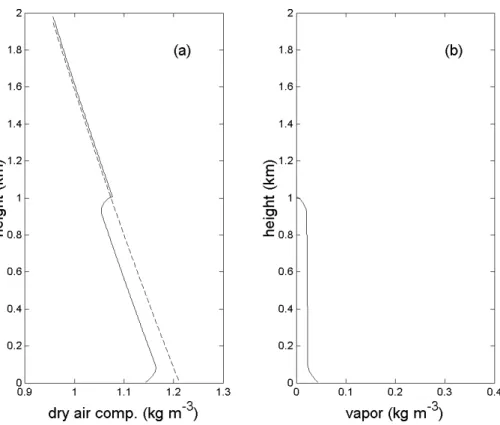
there is only dry air, with its vertical density distributionρd(z) in equilibrium (Fig. 1a). Dry air is treated as a single component for convenience. While the surface is evapo-rating, the local pressure rises slightly, due to the additional vapor molecules, and con-sequently the column above (which still has the same weight) is being shifted slightly.

5

Consequently, the lower layer is expanding – to make room for the water molecules – so that its pressure is brought again in equilibrium with the weight of the column above. A simple calculation shows that for an evaporation rateE=1 mm h−1_{(which is} consid-erable) the lifting velocity will be about 0.4 mm s−1 _if _p

=105Pa and T=288 K. Since the incurred accelerationd w/d t will be very small, it follows from Eq. (2) that during

10

the entire process, hydrostatic equilibrium will be approximately maintained. Note in passing that, on the other hand, condensation would cause compression of the air (neglecting thermal effects).

What are the consequences of the above for the equilibrium of separate compo-nents? Certainly, the water vapor (Fig. 1b) will not reach equilibrium since this would

15

require the water vapor to be taken up to very great height (Eq. 8 with h_v=13.5 km). We agree with M&G that observedρv-profiles are usually compressed vertically with respect to the equilibrium profile. But will the equilibrium for the dry-air profile be pre-served, as M&G claim? Above the boundary layer, the profile is raised to a higher level (Fig. 1a), but density values will still correspond with their original pressure levels,

20

thereby preserving the original profile in a sense. However, within the boundary layer, expansion has occurred to make room for the water molecules added by surface evap-oration and this must have caused the dry-air component to depart from its original equilibrium (according to Eq. 8, Fig. 1a). Thus, a deviation from equilibrium for one component is transferred automatically to another through macroscopic motion, in this

25

case the expansion of the boundary layer. Disequilibrium for one air component can-not coexist for long with equilibrium of the other components, since that would mean (according to Eq. 13) bulk disequilibrium, and hence the initiation of restoring motion.

(11)

HESSD

6, 401–416, 2009

Gorshkov

Title Page

Tables Figures

◭ ◮

Back Close

Full Screen / Esc

Interactive Discussion 3.2 M&G’s approach to evaporation

We have now reached a point at which we can evaluate M&G’s derivation of the “evap-orative force”. It follows from Eqs. (2) and (13) that:

ρd w d z =(−

∂p_d

∂z −ρdg)+(− ∂p_v

∂z −ρvg) (14)

M&G assume stationary motion, so that because of:

5

d w d t =

∂w ∂t +w

∂w

∂z (15)

the left-hand side of Eq. (14) may be replaced by 1₂ρ∂w2/∂z. In the “traditional” view (Sect. 3.1), the vertical velocity w is very low, and therefore the acceleration in the left-hand side of Eq. (14) is very weak. Consequently, the two terms on the right-hand side should almost cancel each other (hence there is bulk-equilibrium). However, at

10

this point M&G assume equilibrium for the dry-air component (Eq. 12) and thus their version of Eq. (14) becomes:

ρd w d t =−

∂p_v

∂z −ρvg (16)

This is M&G’s Eq. (15). As the vapor-disequilibrium on the right-hand side is now – incorrectly – no longer balanced by the dry-air disequilibrium, there is consequently

15

a very strong deviation from bulk-equilibrium which is bound to lead to a very violent restoring motion. A numerical example (M&G’s Eq. 18) yields eventual vertical ve-locities of a much as 50 m s−1_{, considered by them to be “in good agreement with the} maximum updraft velocities observed in typhoons and tornadoes”. However, according to the M&G theory such stationary velocities should be common above any

evaporat-20

ing surface! Naturally, this raises serious questions about the physical realism of the M&G analysis.

(12)

HESSD

6, 401–416, 2009

Gorshkov

Title Page

Tables Figures

◭ ◮

Back Close

Full Screen / Esc

Interactive Discussion violent motions would cause a very rapid expansion of the air column (thereby restoring

bulk-equilibrium) while at the same time disturbing the equilibrium for the dry-air com-ponent. However, M&G imagine an atmosphere in which the dry-air component stays immobile in the presence of (even violent) vertical motion. This logical contradiction leads to an atmosphere in which bulk-equilibrium cannot be restored.

5

It may be elucidating at this point to consider a further thought experiment. Consider a container filled with a boundary layer consisting of dry air, which is then covered with an air-tight lid. Next, water vapor with a realistic vertical profile is added to the container, without lifting the lid. The air cannot expand, due to the closed lid, henceρ_d will remain approximately the same. This will cause a substantial overpressure. Upon

10

pulling the lid, one will initially see a vertical acceleration as described by Eq. (16), but this will be a transient phenomenon as mechanical equilibrium is soon restored.

The strong upward force implied by Eq. (16) is called “evaporative force” by M&G. Because surface evaporation is far too small to provide the very strong upward flow of vapor in the atmosphere presumed by them, M&G argue that lateral inflow of vapor

15

by advection is needed to restore the vapor mass balance. However, a more careful (“traditional”) analysis of the motion associated with evaporation as presented here shows no reason for such a discontinuity. The motion caused by evaporation leads to an expansion of the boundary layer which is just enough to make room for the water vapor added by the evaporation, and this involves no disturbance of the mass balance.

20

The inferred horizontal inflow caused by the “evaporative force” is worked out fur-ther in M&G’s Sect. 3.3. Although the argument remains qualitative for a long time, it would seem that when the estimated vertical velocity is translated to the speed of the horizontal converging currents, wind speeds far in excess of observed values would be obtained. When the M&G analysis finally does become quantitative, the power of the

25

evaporative force is expressed using a new characteristic vertical velocity scalewf. It is pertinent to note that the typical value forwf of 5.6 mm s−1 derived by M&G, is four orders of magnitude smaller than the value given by M&G in their Eq. (18). Apparently this is necessary to bring their theory into agreement with the observations.

(13)

HESSD

6, 401–416, 2009

Gorshkov

Title Page

Tables Figures

◭ ◮

Back Close

Full Screen / Esc

Interactive Discussion 4 Concluding remarks

In this commentary the theoretical basis of the “evaporative force” proposed by Makarieva and Gorshkov (2007, M&G) to explain large-scale precipitation gradients in relation to the presence or absence of forest vegetation has been analyzed in some detail. It is concluded that M&G’s theory is based on an incorrect interpretation of basic

5

physical principles operating in a free atmosphere. However, it should be emphasized that this commentary is more limited in scope than the paper by M&G. For example, it does not address the problems of moisture transport and the spatial distribution of precipitation, as summed up in the valuable introductory part of M&G that draws atten-tion to the various phenomena requiring further study. At the same time, M&G do not

10

do full justice to the existing literature (see for instance Van der Molen et al., 2006); in particular, they ignore such complex spatio-temporal atmospheric flow patterns as the ascending and descending branches of the Hadley Circulation, the shielding e_ffect of mountain ranges, etc., all of which are fundamental to understanding precipitation regimes and vegetation zonation (cf. Walter, 1964; Walter and Lieth, 1967).

15

The question as to whether or not the existence of some kind of “biotic pump” should be invoked, is also outside the scope of this commentary but we do believe with M&G that the role of vegetation – and in particular forest – in generating rainfall is still poorly understood. Likewise, with changes in terrestrial land cover due to deforestation be-ing on the increase, such questions potentially assume added importance. M&G are

20

to be complimented for their valiant attempt to shed more light on the interaction be-tween forest vegetation and precipitation. However, a good understanding of these phenomena should be based on well-founded scientific principles, and not on the kind of ill-conceived ideas which this commentary has shown to be physically untenable.

Acknowledgements. This investigation was funded by the EU WATCH Program.

(14)

HESSD

6, 401–416, 2009

Gorshkov

Title Page

Tables Figures

◭ ◮

Back Close

Full Screen / Esc

Interactive Discussion References

Bruijnzeel, L. A.: Hydrological functions of tropical forests: not seeing the soil for the trees?, Agr. Ecosyst. Environ., 104, 185–228, doi:10.1016/j.agee.2004.01.015, 2004. 402

Costa, M. H.: Large-Scale Hydrological Impacts of Tropical Forest Conversion, in: Forests, Wa-ter and People in the Humid Tropics, edited by: Bonell, M. and Bruijnzeel, L. A., Cambridge

5

University Press, Cambridge, 590–597, 2004. 402

Dill, K. A. and Bromberg, S.: Molecular driving forces, Garland Science, New York, 2003. 406 Dolman, A. J., Silva Dias, M. A. F., Calvet, J-C., Ashby, M., Tahara, A. S., Delire, C., Kabat, P.,

Fisch, G. F., and Nobre, C. A.: Meso-scale effects of tropical deforestation in Amazonia: preparatory LBA modelling studies, Ann. Geophys.-Italy, 17, 1095–1110, 1999. 403

10

Dutton, J. A.: The Ceaseless Wind, an Introduction to the Theory of Atmospheric Motion, Dover Publications, New York, 1986. 407

Gedney, N. and Valdes, P. J.: The effect of Amazonian deforestation on the Northern Hemi-sphere circulation and climate, Geophys. Res. Lett., 27(19), 3053–3056, 2000. 402

Henderson-Sellers, A., Dickinson, R. E., Durbidge, T. B., Kennedy, P. J., McGuffie, K., and

15

Pitman, A. J.: Tropical deforestation – Modeling local-scale to regional-scale climate change, J. Geophys. Res., 98, D4, 7289–7315, 1993. 402

Holton, J. R.: An Introduction to Dynamic Meteorology, 2nd edn., Academic Press, New York, 1979. 407

Landau, L. D. and Lifshitz, E. M.: Course of Theoretical Physics, 6, Fluid Mechanics, Pergamon

20

Press, Oxford, 1987. 404, 405, 406, 408

Makarieva, A. M. and Gorshkov, V. G.: Biotic pump of atmospheric moisture as driver of the hydrological cycle on land, Hydrol. Earth Syst. Sci., 11, 1013–1033, 2007,

http://www.hydrol-earth-syst-sci.net/11/1013/2007/. 403

McEwan, M. J. and Phillips, L. F.: Chemistry of the Atmosphere, Edward Arnold, London, 1975.

25

407

Moore, N., Arima, E., Walker, R., and Ramos da Silva, R.: Uncertainty and the changing hydro-climatology of the Amazon, Geophys. Res. Lett., 34, L14707, doi:10.1029/2007GL030157, 2007.

Nobre, C. A., Sellers, P. J., and Shukla, J.: Amazonian deforestation and regional climate

30

change, J. Climate, 4, 957–988, 1991. 402

Roy, S. B. and Avissar, R.: Impact of land use/land cover change on regional hydrometeorology

(15)

HESSD

6, 401–416, 2009

Gorshkov

Title Page

Tables Figures

◭ ◮

Back Close

Full Screen / Esc

Interactive Discussion in Amazonia, J. Geophys. Res., 107, D20, 8037, doi:10.1029/2001JD000662, 2002. 403

Silva Dias, M. A. F., Rutledge, S., Kabat, P., Silva Dias, P. L., Nobre, C., Fisch, G., Dolman, A. J., Zipser, E., Garstang, M., Manzi, A. O., Fuentes, J. D., Rocha, H. R., Marengo, J., Plana-Fattori, A., S ´a, L. D. A., Alval ´a, R. C. S., Andreae, M. O., Artaxo, P., Gielow, R., and Gatti, L.: Cloud and rain processes in a biosphere atmosphere interaction context in the Amazon

5

Region, J. Geophys. Res., 107, D20, 8072, doi:10.1029/2001JD000335, 2002.

Tennekes, H. and Lumley J. L.: A First Course in Turbulence, The MIT Press, Cambridge MA, 1990. 406

Van Kampen, N. G.: Stochastic Processes in Physics and Chemistry, North Holland Publishing Company, Amsterdam, 1983. 406

10

Van der Molen, M. K., Dolman, A. J., Waterloo, M. J., and Bruijnzeel, L. A.: Climate is affected more by maritime than by continental landuse change: a multiple-scale analysis, Global Planet. Change, 54, 128–149, 2006. 413

Von Hann, J.: Lehrbuch der Meteorologie, Verlag von Christian Hermann Tauchnitz, Leipzig, 1915. 408

15

Wallace, J. M. and Hobbs, P. V.: Atmospheric Sciences, an Introductory Survey, Academic Press, Orlando FL, 1977. 407

Walter, H.: Die Vegetation der Erde in oeko-physiologischer Betrachtung, Fisher, Jena, 1964. 413

Walter, H. and Lieth, H.: Klimadiagramm Weltatlas, Gustav Fisher, Jena, 1967. 413

20

(16)

HESSD

6, 401–416, 2009

Gorshkov

Title Page

Tables Figures

◭ ◮

Back Close

Full Screen / Esc

Interactive Discussion Fig. 1. Illustration of the reaction of a dry boundary layer to evaporation. (a)Dashed line: dry

air mass density, before evaporation. Solid line: the same, after evaporation. (b)Added water vapor mass density (exaggerated).

Comment on &quot;Biotic pump of atmospheric moisture as driver of the hydrological cycle on land&quot; by A. M. Makarieva and V. G. Gorshkov, Hydrol. Earth Syst. Sci., 11, 1013–1033, 2007

HESSD

Comment on “Biotic pump of atmospheric

moisture as driver of the hydrological

cycle on land” by A. M. Makarieva and

V. G. Gorshkov, Hydrol. Earth Syst. Sci.,

11, 1013–1033, 2007

HESSD

HESSD

HESSD

HESSD

HESSD

HESSD

HESSD

HESSD

posi-HESSD

HESSD

HESSD

HESSD

HESSD

HESSD

HESSD

Comment on "Biotic pump of atmospheric moisture as driver of the hydrological cycle on land" by A. M. Makarieva and V. G. Gorshkov, Hydrol. Earth Syst. Sci., 11, 1013–1033, 2007