Productivity of nations: a stochastic frontier approach to TFP decomposition

(1)

P

RODUCTIVITY OF

N

ATIONS

:

A STOCHASTIC FRONTIER APPROACH TO

TFP

DECOMPOSITION

J

ORGE

O. P

IRES

F

ERNANDO

G

ARCIA

Dezembro

de 2004

T

e

x

t

o

s

p

a

r

a

D

i

s

c

u

s

ã

o

(2)

P

RODUCTIVITY OF

N

ATIONS

:

A STOCHASTIC FRONTIER APPROACH TO

TFP

DECOMPOSITION

Jorge O. Pires Fernando Garcia

A

BSTRACT

This paper tackles the problem of aggregate TFP measurement using stochastic frontier analysis (SFA). Data from Penn World Table 6.1 are used to estimate a world production frontier for a sample of 75 countries over a long period (1950-2000) taking advantage of the model offered by Battese & Coelli (1992). We also apply the decomposition of TFP suggested by Bauer (1990) and Kumbhakar (2000) to a smaller sample of 36 countries over the period 1970-2000 in order to evaluate the effects of changes in efficiency (technical and allocative), scale effects and technical change. This allows us to analyze the role of productivity and its components in economic growth of developed and developing nations in addition to the importance of factor accumulation. Although not much explored in the study of economic growth, frontier techniques seem to be of particular interest for that purpose since the separation of efficiency effects and technical change has a direct interpretation in terms of the catch-up debate.

(3)

Os artigos dos Textos para Discussão da Escola de Economia de São Paulo da Fundação Getulio Vargas são de inteira responsabilidade dos autores e não refletem necessariamente a opinião da

FGV-EESP. É permitida a reprodução total ou parcial dos artigos, desde que creditada a fonte.

Escola de Economia de São Paulo da Fundação Getulio Vargas FGV-EESP

www.fgvsp.br/economia

a crucial role in explaining differences in the productivity of developed and developing nations, even larger than the one played by the technology gap.

K

EY

W

ORDS

Total factor productivity, stochastic frontiers, technical change, technical efficiency, allocative efficiency, scale efficiency, convergence

C

LASSIFICAÇÃO

JEL

(4)

1

1 I

I

n

t

r

o

d

u

c

t

i

o

n

This paper uses an alternative way of measuring total factor productivity based on the analysis of stochastic frontiers. The great advantage of this approach is the possibility that it offers of decomposing productivity change into parts that can have a straightforward and simple economic interpretation. The stochastic frontier model used assumes the existence of technical inefficiency which evolves following a particular behavior. These assumptions allow one to split productivity changes into two parts. The first is the change in technical efficiency, which measures the movement of an economy towards the production frontier; the second is technical progress, which measures shifts of the frontier over time.

When applied to a flexible technology (e.g.: translog) – this technique further allows one to evaluate the presence of scale efficiency. The Bauer-Kumbhakar decomposition is then applied to a sample of 36 countries from 1970 to 2000, allowing the additional measurement of changes in allocative efficiency. The relative magnitude of this last component (allocative efficiency), together with technical change, seem to explain a large portion of the differences in economic growth between developed and developing countries.

(5)

2

2 T

T

h

e

s

t

o

c

h

a

s

t

i

c

f

r

o

n

t

i

e

r

a

n

d

T

F

P

d

e

c

o

m

p

o

s

i

t

i

o

n

The model used is basically that developed in the literature on technical efficiency and productivity, more specifically in the “statistical” and “parametric” branches of this literature, and is known as Stochastic Frontier Analysis (SFA). The focus of SFA is to obtain an estimator for one of the components of TFP, the degree of technical efficiency. Technical efficiency is estimated in addition to technical change which in its turn is captured (as usual) by a time trend and interactions of the regressors with time. The model used here is essentially that developed (independently) by Aigner, Lovell & Schmidt (1977) and by Meeusen & van den Broeck (1977). Their formulation was extended by Pitt & Lee (1981) and Schmidt & Sickles (1984) for the panel data case. Since then a number of enhancements have been suggested, such as that of Battese & Coelli (1992), in which the technical inefficiency is modeled so as to be time variant.

The general stochastic production frontier model is described by the equations below, where y is the vector for the quantities produced by the various countries, x is the vector for production factors used and β is the vector for the parameters defining the production technology.

) u exp( ) v exp( ) , x , t ( f

y= β ⋅ ⋅ − , u ≥ 0 (1)

The v and u terms (vectors) represent different error components. The first refers to the random part of the error, while the second represents technical inefficiency, i.e., the part that is a downward deviation from the production frontier (which can be inferred by the negative sign and the restriction u≥0). Thus, f(t,x,β)⋅exp(v) represents the frontier of stochastic production and

v has a symmetrical distribution to capture the random effects of measuring errors and exogenous shocks that cause the position of the deterministic nucleus of the frontier, f(t,x,β), to vary from country to country. The technical inefficiency is captured by the error component exp(−u). For each country i and each time period t, we have:

) u exp( ) v exp( ) , x , t ( f

(6)

Once it is assumed that v~iidN(0,σ2); )u~NT(µ,σ2_u i.e., u has a normal-truncated distribution (with a nonnull average µ)1

; the two error components are independent of each other and x is supposed exogenous, the model can be estimated by maximum-likelihood techniques. Given these conditions, the traditional asymptotic properties of the MV estimators hold. In addition, we take the technical inefficiency component as time-variant, according to parametrization formulated by Battese & Coelli (1992)2:

[

]

i

it exp (t T) u

u = −η − ⋅ , 0u_it ≥ e i=1,...,N e t∈τ(i) (3) In the above expression, τ(i) represents the Ti periods of time for which we have

available observations for the i-nth country, among the available T periods in the panel (i.e., τ(i) may contain all periods in the panel or only a subset of periods). The sign of η dictates the behaviour of technical inefficiency over time. When η is not significantly different from zero, we have technical inefficiency that does not vary in time, also called persistent inefficiency. This specification of the behavioral pattern of inefficiency is somewhat inflexible, as the model’s architects themselves admit, for, according to the formulation, technical inefficiency must grow at decreasing rates (η>0), or decrease at increasing rates (η<0). Moreover, the estimated value for η is the same for all countries in the sample, which means to say that the pattern of inefficiency rise or reduction is the same for all countries.

Assuming a translog technology with two production factors, namelly capital (K) and labor (L), the model can be expressed in the following way:

[

it

]

Lt

[

it

]

it it Kt it it KL 2 it LL 2 it KK 2 tt it L it K t 0 it u v t ) L (ln t ) K (ln ) L (ln ) K (ln 2 1 ) L (ln 2 1 ) K (ln 2 1 t . 2 1 L ln K ln t . y ln − + ⋅ β + ⋅ β + ⋅ β + + β + β + β ⋅ + β + β + β + β = (4) 1

The restriction of a half-normal distribution µ=0 can be tested.

2

(7)

The output elasticities with respect to K and L can be obtained from (4), working out the derivatives. Due to the use of a translog technology these elasticities are country and time specific. The technical progress measure is also specific for each country and period of time and can be obtained by time differentiation of (4).

Bauer (1990) and Kumbhakar (2000) suggested a quite ingenious, yet simple, type of productivity decomposition which goes beyond the division of productivity changes into a catch-up effect and a technical innovation effect. Such framework also accounts for scale of production effects and inefficient allocation of productive factors. To perform this decomposition, first of all we must estimate the model depicted by (3) and (4). Once this model is estimated, it is possible to “compose” the rate of total factor productivity change from the results. The components of productivity can be identified from algebraic manipulations from the expression that denotes the deterministic part of the production frontier combined with the usual expression for the the productivity change Divisia index:

L L s K K s y y

g_PTF=& − _K & − _L &

From the deterministic part of (2) we have:

t u L L K K t ) , L , K , t ( f ln y y L K ∂ ∂ − ε + ε + ∂ β ∂

= & &

&

In the expressions above and those that follow, the terms sK and sL represent the shares of

capital and labor in income; εK and εL are output elasticities, with RTS=εK +εL, RTS denoting

the returns to scale; gK and gL are the growth rates of K and L, respectively.

RTS K K ε = λ , RTS L L ε =

λ .

Substituting this result in the expression for the Divisia index, and after some algebraic manipulations we have:

(

)

[

K K L L

]

[

(

K K

)

K

(

L L

)

L

]

PTF PT u RTS 1 g g s g s g

g = −&+ − ⋅ λ ⋅ +λ ⋅ + λ − ⋅ + λ − ⋅ (5)

(8)

(i) the technical progress, measured by

t ) , L , K , t ( f ln TP

∂ β ∂

= ;

(ii) the change in technical efficiency, denoted by u−&;

(iii) the change in the scale of production, given by

(

RTS−1

)

⋅

[

λ_K⋅g_K+λ_L⋅g_L

]

; and

(iv) the change in allocative efficiency, measured by

(

)

(

)

[

λK −sK ⋅gK+ λL −sL ⋅gL

]

.

We can then study the impact of each of the components of TFP. If the technology is immutable, it does not contribute in any way to productivity gains. The same happens with technical inefficiency. If it does not vary in time, it also does not have any impact on the rate of variation of productivity.

The contribution of economies of scale depends both on technology as well as on factor accumulation. If there are constant returns to scale, then RTS = 1, which cancels out the third component of the productivity variation. Otherwise, if RTS ≠ 1, part of the productivity change is explained by changes in the scale of production. In the case of increasing returns to scale (RTS > 1) and an increase in the amount of productive factors we have a higher rate of productivity growth. If the amounts of production factors diminish, then we would have a reduction in the rate of productivity change. An inverse analogous reasoning can be made for decreasing returns and reduction (increase) in the amount of productive factors.

(9)

3

3 D

D

a

t

a

n

d

s

a

m

p

l

e

The database for this study consists of a non-balanced panel for aggregated output and production factors (K and L) of a sample of countries that includes both wealthy as well as poor nations. These data were basically obtained from Penn World Tables (PWT), version 6.1, for years 1950 to 2000. Below we detail the definitions of each series used in the econometric estimations We also describe the procedures used in selecting the countries and the time periods that actually comprise the econometric estimations.

The output variable is GDP measured at constant prices (1996 US$), with purchasing power parity (PPP) adjustment. It is obtained by taking the real GDP per capita chain series

(RGDPPCH) from PWT 6.1 and multiplying it by total population for each country.

With respect to labor we use a proxy, the population of equivalent adults (peqa), obtained from PWT. The concept derives from population data: based on data for the total population, an average is computed that attributes a weight of 1 to people older than 15 and 0.5 to people aged up to 15 (pop>15 * 1 + pop<=15*0.5). These data are obtained indirectly from the PWT 6.1, by performing calculations using three variables: real GDP per capita chain series (rgdpch) was divided by real GDP per equivalent adult (rgdpeqa) and then multiplied by the population (pop):

pop GDP

peqa pop

GDP pop

rgdpeqa rgdpch

L = ⋅ = ⋅ ⋅

Another possibility would be to use data pertaining to the labor force. These can be obtained through a transformation similar to the one described above, using the variable real

GDP per worker (rgdpwok). Detailed analysis of the two series per country suggests that the peqa

series is more reliable, which was the motivation of our choice.

The perpetual inventory method was used to compute a series for the stock of capital of each nation in the sample3. This method uses an initial capital stock estimate (computed from investment data), the supposition of a stable rate of growth for a given period, and additional

3

(10)

suppositions regarding the depreciation rate. The measure of the initial capital stock is quite sensitive to the problems of measurement error regarding the flow of investment (and also the growth of GDP).

The investment series used in computing the capital stock was obtained from multiplying the GDP, in constant 1996 local currency, by the “current” investment rate, and then converting this result to US$ using the 1996 exchange rate. GDP in 1996 local currency units was obtained by simply adding up all its components, which are available in the nafinalpwt spreadsheet of the PWT. The current investment rate was obtained dividing the value of investment in current local currency by the current GDP. The exchange rate used is obtained from the series XRAT, found in

the nafinalpwt spreadsheet of the PWT 6.1.

The initial capital stock is computed using the investment series. To do so, we took as the reference year, the year following that of the start of the investment series. We then used the perpetual inventory method to build up the remainder of the series. This procedure allowed each country to have its own capital stock series beginning in the first year for which we have available data for aggregated investment.

The capital stock series used in this study was not adjusted for purchasing power parity disparities. More specifically it is taken in constant 1996 US$. This reflects the perception that investment decisions are taken considering relative domestic prices. Cohen & Soto (2003) also notice this and argue that PPP adjustment imposes on poorer countries relative prices that are different from those of the market, and an apparently high marginal productivity of capital. The price of investment goods has been decreasing over time in relation to the price of other products, a trend that has become more evident with the growing production of the information technology and communications industries. The quality of the products in these two industries has undoubtedly been improving, with prices continually dropping and capital use continually increasing. The consequence of this is that the importance of factor accumulation in the explanation of economic growth is increasing, making the part relative to productivity smaller. Once capital stock values undergo PPP adjustment, these effects are exacerbated.

Factor shares sK and sL were basically obtained from two databases: (i) the Annual

(11)

United Nation’s System of National Accounts (SNA68). For OECD nations belonging to the sample in this study, we have used only this organization’s database (it is homogeneous and contains more information than the SNA, some of them estimates, though). Information pertaining to other nations, not OECD members, were obtained mostly from SNA68.

Data for some countries were not available in SNA68 (usually those pertaining to the first and the last years of the sample). For these countries we tried other sources. Among them we can name ECLAC (Economic Commission for Latin America and the Caribeean) for data pertaining to Bolivia (2000), Costa Rica4 (2000), Trinidad & Tobago (2000) and Jamaica and Peru (1995 and 2000), and MIDEPLAN (Ministerio de Planificación y Cooperación) for Chile (1975 to 1985 and 2000) 5. For Brazil, data used are from the local official statistical bureau (IBGE).

The selection of countries included in the sample followed some criteria. The first and obvious criterion was availability of homogeneous data for the period in question. Nations that had a reduced number of observations were excluded. A minimum number of 30 continuous observations per country was set. Therefore, of the 203 economies listed in the PWT 6.1, 86 countries that did not have information on either the labor force, GDP, investment, or exchange rate for the last 30 years were excluded. This criterion essentially removed from the sample a number of countries created or split in the last 20 to 30 years.

Previously socialist economies, such as People’s Republic of China, Hungary, Romania and Poland, or those nations that are protectorates of others, such as Puerto Rico and Taiwan6, were also excluded. The group of 86 excluded nations also includes those with a very small population – less than 500 thousand inhabitants in 2000. For this reason countries like Barbados, Cape Verde, Equatorial Guinea, Luxembourg and Seychelles Islands were also left out. The only exception to this last rule was Iceland, a country with (“good quality”) information dating back to 1950.

4

For Bolivia and Costa Rica the numbers for 2000 are actually those of 1999.

5

For Chile, there was no available information for 1970 in any sources used. We used then the numbers for 1973, first year for which the national accounts of this country displays that information.

(12)

Of the remaining 112 economies, another 13 were excluded because of lapses in the historical series caused by wars, civil wars or split-ups. In these cases, the estimation of capital stock using the perpetual inventory processes can clearly not be applied. The countries rejected due to this criterion were the following: Angola, Ethiopia, Bangladesh, Guinea, Comoros, Haiti, Burundi, Central African Republic, Madagascar, Mozambique, Sierra Leone, Papua New Guinea and Zaire (presently Congo). Eighteen other nations were excluded because of having highly volatile GDP per capita and investment rate figures, which causes excessively high deviations in the capital stock estimations (namely, Algeria, Benin, Botswana, Burkina Faso, Cameron, Congo Republic, Ivory Costa, Fiji Islands, Mauritius Islands, Gambia, Guinea Bissau, Guyana, Mali, Mauritania, Namibia, Niger, Tanzania and Togo).

Note that all countries included in this last group are poor, most of them from Africa. A question could be raised here, arguing that this decision would create a biased analysis through selection. We argue that this is not a problem in this study, because the purpose here is to describe a quite flexible production frontier (translog): in this case, output elasticities with respect to the productive factors can vary among countries and in time, which renders flexibility to the adjustments. In the event we undertook an analysis using the Cobb-Douglas technology, elasticities would be constant and would express sample averages subject to selection bias. In this analysis, quite to the contrary, the selection should favor precise estimations, because the excluded economies (due to unreliable data) generally have a low “grade” in the ranking brought by the PWT in regard to data quality.7

This leaves us with 75 countries with data spanning from 1950 to 2000. The observations were taken for 11 different time periods, every 5 years, starting in 1950 and finishing in 2000. This type of procedure is rather common in the economic growth literature and is justified by the interest of studying long-term effects, and this can be perfectly addressed by more spaced time observations. Forbes (2000), to give one example, makes estimations with data gathered every five years and justifies this saying that yearly data contain short-term disturbances. Before proceeding to the estimations, the data were carefully reviewed, on a country per country basis.

7

See Table A, from Data Appendix for a Space-Time System of National Accounts: Penn World Table 6.1

(13)

Special care was taken with the series for capital stock. It is known that estimations for initial capital stock can present problems that render capital stock data for the first years of the series less reliable. We must remember that the initial capital stock calculations presume a stable behavior for the economic growth rate (steady state), an assumption not very realistic. In the event the growth rate for the initial period is too low (much lower than that of steady state), the initial capital stock tends to be overestimated, and consequently these data appear to be reduced in the initial periods. The opposite can occur when the rate is high. Based on scatter plots (capital x GDP) we noticed the presence of observations for some countries that could suggest inadequate estimations of initial capital stock. This was the case of the following countries: Argentina, Australia, Denmark, Iceland, the Netherlands, New Zealand and Syria. Therefore, the first two (or three) observations of the series pertaining these countries were eliminated.

A similar problem occurred for some countries when scatter plots of production and population of equivalent adults were analyzed. Ireland, Greece and Cyprus experienced, at different moments, considerable reductions in their population of equivalent adults, presenting a behavior not compatible with the premise of factors diminishing returns. For the first two nations, this happened at the beginning of the series, a fact that could indicate problems with different sources for population data (up to 1960 the PWT’s population data come from the United Nations

Development Centre and after this year they come from the World Bank). Consequently, we

decided to exclude the first two observations of the series for Ireland (1950 and 1955) and the first (1955) for Greece.

4

4 E

E

s

t

i

m

a

t

i

o

n

o

f

t

h

e

w

o

r

l

d

s

t

o

c

h

a

s

t

i

c

f

r

o

n

t

i

e

r

(

1

9

5

0

0 -

-

2

0

0 )

)

(14)

Parameters presented in Table 1 are all significant at 5%, except the capital elasticity, which is significant at 6.5%. The mean inefficiency, µ, is significantly different from zero at 1%, showing that the normal truncated distribution is an appropriate assumption (if it were not significant, we would fall back to the case of half-normal distribution). The estimated value of η is positive, which means that technical efficiency grows at decreasing rates (catch-up).

βkn is negative, revealing the possibility of substitution between the production factors.

The βt and βtt coefficients indicate that the neutral part of technical progress has negative effects

on production and in order to achieve (positive) technical progress, it is necessary that the non-neutral part of technical progress offsets these effects. The signs of βkt and βnt indicate,

respectively, that the non-neutral part of the technical progress goes hand in hand with the capital accumulation (positive sign of βkt), and inversely with labor supply (negative sign of βnt), i.e.,

technical progress is labor-saving and is more intense in countries where capital is abundant.

Table 1 Time-variant inefficiency model

No. of observations = 746 Observations per country: min = 3 No. of countries = 75 Average = 9.9 Maximum = 11 Log likelihood = 272.07096 Wald χ2(8)= 14,540.41 Prob > χ2 = 0.0000 Confidence interval 95% lny Coefficients Standard error z P>z

lower upper

t -0.1198 0.0455 -2.6300 0.0080 -0.2089 -0.0307 k 0.2457 0.1330 1.8500 0.0650 -0.0149 0.5064 n 0.3767 0.1883 2.0000 0.0450 0.0077 0.7458 tt -0.0075 0.0015 -5.1300 0.0000 -0.0103 -0.0046 kk 0.0275 0.0111 2.4900 0.0130 0.0058 0.0492 nn 0.0572 0.0216 2.6500 0.0080 0.0150 0.0995 kn -0.0605 0.0272 -2.2200 0.0260 -0.1138 -0.0072 kt 0.0106 0.0023 4.6100 0.0000 0.0061 0.0152 nt -0.0063 0.0030 -2.1100 0.0350 -0.0121 -0.0004 0 8.8115 1.8366 4.8000 0.0000 5.2119 12.4111

µ 0.2074 0.0626 3.3100 0.0010 0.0846 0.3302

η 0.0652 0.0116 5.5900 0.0000 0.0423 0.0880 ln σ2 -2.7946 0.2291 -12.2000 0.0000 -3.2437 -2.3456 ilgt 0.6735 0.3514 1.9200 0.0550 -0.0153 1.3623

σ2

0.0611 0.0140 0.0390 0.0958

0.6623 0.0786 0.4962 0.7961

σu2 0.0405 0.0140 0.0131 0.0679

(15)

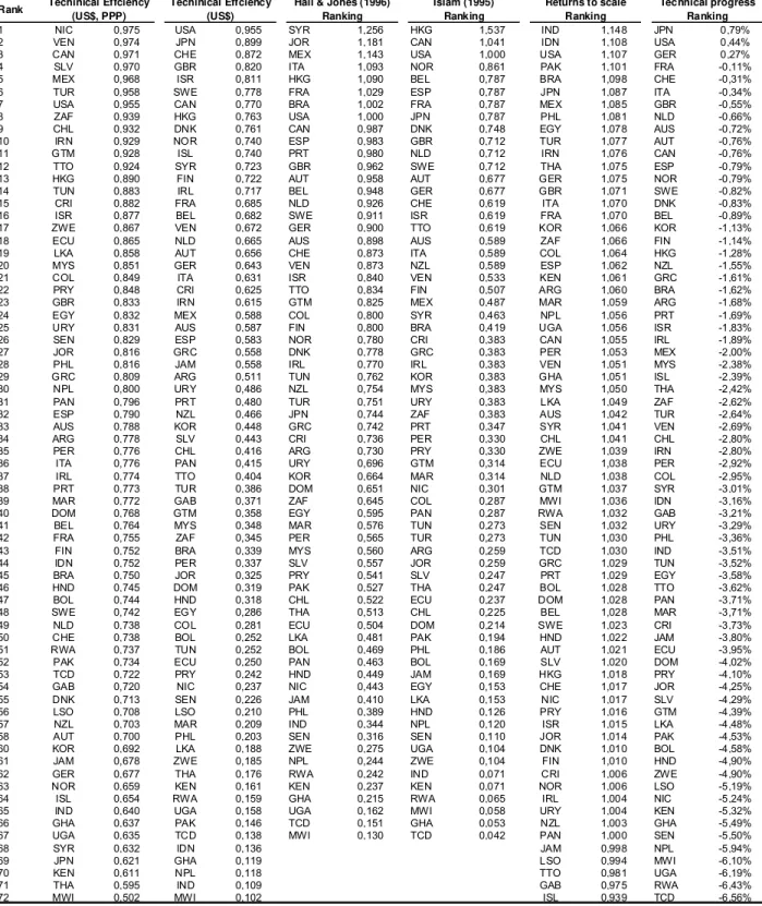
Inspection of the results for returns to scale, technical change, and technical efficiency reveals that these are economically meaningful. Table 2 shows country ranks for RTS, TE, and TP. The technical efficiency ranking must be viewed with caution. Although the presence of countries like Nicaragua, Venezuela and El Salvador in the first positions of the ranking does indeed seem odd, two aspects must be kept in mind: (i) these results are “conditional” on the capital-labor ratio; and (ii) the estimations took place using PPP adjusted figures for GDP. In other words, the first aspect mentioned means that, in a traditional Farrel diagram, a country such as Nicaragua is closer to the frontier, yet it is placed at the “edge” of the unit isoquant closest to the axis of the labor factor, at the same time that a country like Norway would be further from the frontier, but on the opposite edge of the isoquant (abundant capital, scarce labor).

(16)

Table 2. Technical efficiency, returns to scale and technical progress, 2000

Rank

1 NIC 0,975 USA 2 VEN 0,974 JPN 3 CAN 0,971 CHE 4 SLV 0,970 GBR 5 MEX 0,968 ISR 6 TUR 0,958 SWE 7 USA 0,955 CAN 8 ZAF 0,939 HKG 9 CHL 0,932 DNK 10 IRN 0,929 NOR 11 GTM 0,928 ISL 12 TTO 0,924 SYR 13 HKG 0,890 FIN 14 TUN 0,883 IRL 15 CRI 0,882 FRA 16 ISR 0,877 BEL 17 ZWE 0,867 VEN 18 ECU 0,865 NLD 19 LKA 0,858 AUT 20 MYS 0,851 GER 21 COL 0,849 ITA 22 PRY 0,848 CRI 23 GBR 0,833 IRN 24 EGY 0,832 MEX 25 URY 0,831 AUS 26 SEN 0,829 ESP 27 JOR 0,816 GRC 28 PHL 0,816 JAM 29 GRC 0,809 ARG 30 NPL 0,800 URY 31 PAN 0,796 PRT 32 ESP 0,790 NZL 33 AUS 0,788 KOR 34 ARG 0,778 SLV 35 PER 0,776 CHL 36 ITA 0,776 PAN 37 IRL 0,774 TTO 38 PRT 0,773 TUR 39 MAR 0,772 GAB 40 DOM 0,768 GTM 41 BEL 0,764 MYS 42 FRA 0,755 ZAF 43 FIN 0,752 BRA 44 IDN 0,752 PER 45 BRA 0,750 JOR 46 HND 0,745 DOM 47 BOL 0,744 HND 48 SWE 0,742 EGY 49 NLD 0,738 COL 50 CHE 0,738 BOL 51 RWA 0,737 TUN 52 PAK 0,734 ECU 53 TCD 0,722 PRY 54 GAB 0,720 NIC 55 DNK 0,713 SEN 56 LSO 0,708 LSO 57 NZL 0,703 MAR 58 AUT 0,700 PHL 60 KOR 0,692 LKA 61 JAM 0,678 ZWE 62 GER 0,677 THA 63 NOR 0,659 KEN 64 ISL 0,654 RWA 65 IND 0,640 UGA 66 GHA 0,637 PAK 67 UGA 0,635 TCD 68 SYR 0,632 IDN 69 JPN 0,621 GHA 70 KEN 0,611 NPL 71 THA 0,595 IND 72 MWI 0,502 MWI 0,955 SYR 1,256 HKG 1,537 IND 1,148 JPN 0,79% 0,899 JOR 1,181 CAN 1,041 IDN 1,108 USA 0,44% 0,872 MEX 1,143 USA 1,000 USA 1,107 GER 0,27% 0,820 ITA 1,093 NOR 0,861 PAK 1,101 FRA -0,11% 0,811 HKG 1,090 BEL 0,787 BRA 1,098 CHE -0,31% 0,778 FRA 1,029 ESP 0,787 JPN 1,087 ITA -0,34% 0,770 BRA 1,002 FRA 0,787 MEX 1,085 GBR -0,55% 0,763 USA 1,000 JPN 0,787 PHL 1,081 NLD -0,66% 0,761 CAN 0,987 DNK 0,748 EGY 1,078 AUS -0,72% 0,740 ESP 0,983 GBR 0,712 TUR 1,077 AUT -0,76% 0,740 PRT 0,980 NLD 0,712 IRN 1,076 CAN -0,76% 0,723 GBR 0,962 SWE 0,712 THA 1,075 ESP -0,79% 0,722 AUT 0,958 AUT 0,677 GER 1,075 NOR -0,79% 0,717 BEL 0,948 GER 0,677 GBR 1,071 SWE -0,82% 0,685 NLD 0,926 CHE 0,619 ITA 1,070 DNK -0,83% 0,682 SWE 0,911 ISR 0,619 FRA 1,070 BEL -0,89% 0,672 GER 0,900 TTO 0,619 KOR 1,066 KOR -1,13% 0,665 AUS 0,898 AUS 0,589 ZAF 1,066 FIN -1,14% 0,656 CHE 0,873 ITA 0,589 COL 1,064 HKG -1,28% 0,643 VEN 0,873 NZL 0,589 ESP 1,062 NZL -1,55% 0,631 ISR 0,840 VEN 0,533 KEN 1,061 GRC -1,61% 0,625 TTO 0,834 FIN 0,507 ARG 1,060 BRA -1,62% 0,615 GTM 0,825 MEX 0,487 MAR 1,059 ARG -1,68% 0,588 COL 0,800 SYR 0,463 NPL 1,056 PRT -1,69% 0,587 FIN 0,800 BRA 0,419 UGA 1,056 ISR -1,83% 0,583 NOR 0,780 CRI 0,383 CAN 1,055 IRL -1,89% 0,558 DNK 0,778 GRC 0,383 PER 1,053 MEX -2,00% 0,558 IRL 0,770 IRL 0,383 VEN 1,051 MYS -2,38% 0,511 TUN 0,762 KOR 0,383 GHA 1,051 ISL -2,39% 0,486 NZL 0,754 MYS 0,383 MYS 1,050 THA -2,42% 0,480 TUR 0,751 URY 0,383 LKA 1,049 ZAF -2,62% 0,466 JPN 0,744 ZAF 0,383 AUS 1,042 TUR -2,64% 0,448 GRC 0,742 PRT 0,347 SYR 1,041 VEN -2,69% 0,443 CRI 0,736 PER 0,330 CHL 1,041 CHL -2,80% 0,416 ARG 0,730 PRY 0,330 ZWE 1,039 IRN -2,80% 0,415 URY 0,696 GTM 0,314 ECU 1,038 PER -2,92% 0,404 KOR 0,664 MAR 0,314 NLD 1,038 COL -2,95% 0,386 DOM 0,651 NIC 0,301 GTM 1,037 SYR -3,01% 0,371 ZAF 0,645 COL 0,287 MWI 1,036 IDN -3,16% 0,358 EGY 0,595 PAN 0,287 RWA 1,032 GAB -3,21% 0,348 MAR 0,576 TUN 0,273 SEN 1,032 URY -3,29% 0,345 PER 0,565 TUR 0,273 TUN 1,030 PHL -3,36% 0,339 MYS 0,560 ARG 0,259 TCD 1,030 IND -3,51% 0,337 SLV 0,557 JOR 0,259 GRC 1,029 TUN -3,52% 0,325 PRY 0,541 SLV 0,247 PRT 1,029 EGY -3,58% 0,319 PAK 0,527 THA 0,247 BOL 1,028 TTO -3,62% 0,318 CHL 0,522 ECU 0,237 DOM 1,028 PAN -3,71% 0,286 THA 0,513 CHL 0,225 BEL 1,028 MAR -3,71% 0,281 ECU 0,504 DOM 0,214 SWE 1,023 CRI -3,73% 0,252 LKA 0,481 PAK 0,194 HND 1,022 JAM -3,80% 0,252 BOL 0,469 PHL 0,186 AUT 1,021 ECU -3,95% 0,250 PAN 0,463 BOL 0,169 SLV 1,020 DOM -4,02% 0,242 HND 0,449 JAM 0,169 HKG 1,018 PRY -4,10% 0,237 NIC 0,443 EGY 0,153 CHE 1,017 JOR -4,25% 0,226 JAM 0,410 LKA 0,153 NIC 1,017 SLV -4,29% 0,210 PHL 0,389 HND 0,126 PRY 1,016 GTM -4,39% 0,209 IND 0,344 NPL 0,120 ISR 1,015 LKA -4,48% 0,203 SEN 0,316 SEN 0,110 JOR 1,014 PAK -4,53% 0,188 ZWE 0,275 UGA 0,104 DNK 1,010 BOL -4,58% 0,185 NPL 0,244 ZWE 0,104 FIN 1,010 HND -4,90% 0,176 RWA 0,242 IND 0,071 CRI 1,006 ZWE -4,90% 0,161 KEN 0,237 KEN 0,071 NOR 1,006 LSO -5,19% 0,159 GHA 0,215 RWA 0,065 IRL 1,004 NIC -5,24% 0,158 UGA 0,162 MWI 0,058 URY 1,004 KEN -5,32% 0,146 TCD 0,151 GHA 0,053 NZL 1,003 GHA -5,49% 0,138 MWI 0,130 TCD 0,042 PAN 1,000 SEN -5,50% 0,136 JAM 0,998 NPL -5,94% 0,119 LSO 0,994 MWI -6,10% 0,118 TTO 0,981 UGA -6,19% 0,109 GAB 0,975 RWA -6,43% 0,102 ISL 0,939 TCD -6,56%

Techinical Effciency (US$)

Returns to scale Ranking Techinical Effciency (US$, PPP) Technical progress Ranking Islam (1995) Ranking Hall & Jones (1996)

(17)

An interesting exercise is to compare our ranking to the productivity indices suggested by Islam (1995) and Hall & Jones (1996). The index of adjusted technical efficiency seems better suited for such comparisons, because it displays the efficiency in US$. This index is highly correlated8 with those suggested by the above authors, with the advantage that this ordering seems to be more intuitive. The less productive nations remain practically unchanged at the bottom of the ranking, but the top of the productivity ranking no longer brings less developed nations, as in Hall & Jones (1996), for whom countries like Syria, Jordan, Mexico and Brazil are listed among the most productive economies, or as in Islam (1995), in which Hong Kong is considered the most productive nation – 53.7% more productive than the United States!

The results for RTS are very intuitive. The countries at the top of the ranking depict increasing returns to scale. These are large countries from the population and territorial perspective. The bottom positions in the ranking are occupied by basically very small (in size and population) countries. Another fact that comes to our attention is that Germany, Great-Britain, Italy and France, all of them European nations of very homogeneous characteristics, are placed next each other in the ranking.

The results for technical progress seem at first sight rather odd, with almost all of them being negative. Nonetheless, the ordering seems to match our intuition regarding the technological performance of the nations. At the top positions are Japan, United States, Germany and France. Among the countries at the bottom are the African nations, well-known for their lack of technological knowledge. A simple exercise of “casual empiricism” provides an interesting “test” of the existence of “economic intuition” behind the estimations of technical progress performed by the model. The idea is to evaluate if the measure of technical progress produced is related in any way to the effort to innovate carried out by countries in recent years. The scatter diagram for the technical progress measure and the natural logarithm of R&D expenses (average

8

(18)

for 1990-2000) show us what seems to be, at least at first sight, a positive relation between these variables.

Graph 1. Expenditures in R&D, human capital and technical progress, 2000

R&D expenditures (Millions of US$) - average 1990-2000 300 .0 00 20 0.00 0 100 .00 0 50_.00 0 40_.00 0 30_.00 0 20 .0₀₀ 10.₀₀₀ 5.000 4.0 00 3.0 00 2.₀₀ 0 1.0 00 50₀ 40₀ 30₀ 20 0 10₀ 50 40 30 20 10 T ec hni cal P rogr es s ( % p. a. ) ,01 0,00 -,01 -,02 -,03 -,04 -,05 VEN USA THA SWE PRT PHL MYS MEX KOR JPN ITA ISL IND GER DNK CHL CHE BRA AUS ARG

Average years of schooling of population over 25 years

14,0 12,0 10,0 8,0 6,0 4,0 2,0 0,0 T ec hni cal pr ogr es s ( % p. a. ) ,0 0,0 -,0 -,0 -,1 -,1 ZWE VEN USA UGA THA SWE SEN PRT PHL PAK MYS MEX LSO KOR JPN ITA ISL IND GER FRA ESP DNK COL CHL CHE BRA AUS ARG

Fonte: Table 2 and WDI 2002.

Another similar diagram, but relating the measure of technical progress with the average education level of the population shows another intuitive relation: countries with better educated population are also the ones with the highest levels of technical progress.

(19)

to have higher variance of technical efficiency and lower of technical progress (which comes out negative for all countries after 1997). For this reason, the influence of µ in the total variance also rises, from 66.3% to 77%. If the estimation of the technical inefficiency were based on the Battese & Coelli (1995) model, maybe it would be possible to control the effect of these short-term variations.

The estimates produced by the fixed-effects and random-effects models in turn came out quite inferior to those of the stochastic frontier models. The Hausman test (χ2

= 49,03) favors the fixed effects model, although 4 out the 9 coefficients of the translog specification ended up being not significant at 10%. Furthermore, the results are not intuitive at all. Some countries have zero or negative labor elasticities, such as Iceland and South Korea, and the returns to scale vary greatly: the United States, to give an example, would have an estimated RTS of 1.26, whereas Iceland would be a mere 0.49. The estimations of technical progress likewise are not very reasonable: United States, Japan and Germany show large technical regress at the same time that Trinidad & Tobago, Lesotho and Jamaica have extraordinary technical progress. This result reinforces the idea that frontier models are better suited for the analysis of productivity in comparison with traditional econometric methods.

5

5 T

T

F

P

a

n

d

i

t

s

c

o

m

p

o

n

e

n

t

s

(

1

9

7

0

0 -

-

2

0

0 )

)

With the results of the estimation of the model, obtained in Section 3 for the 75 countries of the sample, and the data on functional income distribution (sK and sL), it is possible to

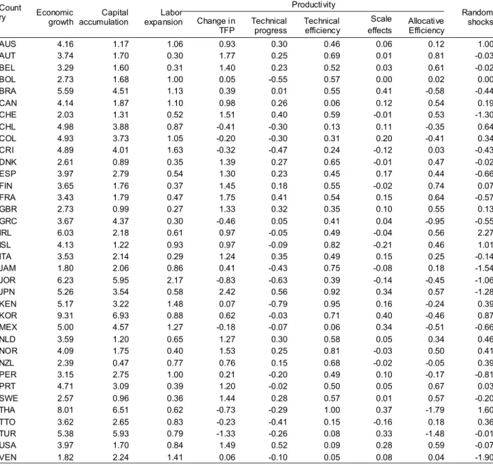
decompose productivity change in the manner shown in section 1. However data for factors shares in income are not available for all these economies. We managed to collect data for only 36 of the 75 countries, and just from 1970 up to 2000. The “full” decomposition of TFP is then restrict to this group of 36 nations. Table 3 brings the results.

(20)

countries are Austria (1.77%), France (1.75%), Norway (1.53%), Switzerland (1.51%) and USA (1.49%). In the middle block we find some Latin American countries, such as Jamaica, Brazil, Peru, Venezuela and Bolivia, all of them with relatively low TFP growth rates. Brazil showed during this period an average rise in productivity of 0.39% per year. Among the other Latin American countries of the sample we see that Mexico, Costa Rica, and, surprisingly, Chile had reductions in productivity. Greece and Turkey are the only OECD members with negative productivity growth during this time.

(21)

Table 3. Sources of economic growth 1970-2000 – average annual change in (%)

Productivity Count

ry Economic growth

Capital accumulation

Labor

expansion Change in TFP

Technical progress

Technical efficiency

Scale effects

Allocative Efficiency

Random shocks

AUS 4.16 1.17 1.06 0.93 0.30 0.46 0.06 0.12 1.00 AUT 3.74 1.70 0.30 1.77 0.25 0.69 0.01 0.81 -0.03 BEL 3.29 1.60 0.31 1.40 0.23 0.52 0.03 0.61 -0.02 BOL 2.73 1.68 1.00 0.05 -0.55 0.57 0.00 0.02 0.00 BRA 5.59 4.51 1.13 0.39 0.01 0.55 0.41 -0.58 -0.44 CAN 4.14 1.87 1.10 0.98 0.26 0.06 0.12 0.54 0.19 CHE 2.03 1.31 0.52 1.51 0.40 0.59 -0.01 0.53 -1.30 CHL 4.98 3.88 0.87 -0.41 -0.30 0.13 0.11 -0.35 0.64 COL 4.93 3.73 1.05 -0.20 -0.30 0.31 0.20 -0.41 0.34 CRI 4.89 4.01 1.63 -0.32 -0.47 0.24 -0.12 0.03 -0.43 DNK 2.61 0.89 0.35 1.39 0.27 0.65 -0.01 0.47 -0.02 ESP 3.97 2.79 0.54 1.30 0.23 0.45 0.17 0.44 -0.66 FIN 3.65 1.76 0.37 1.45 0.18 0.55 -0.02 0.74 0.07 FRA 3.43 1.79 0.47 1.75 0.41 0.54 0.15 0.64 -0.57 GBR 2.73 0.99 0.27 1.33 0.32 0.35 0.10 0.55 0.13 GRC 3.67 4.37 0.30 -0.46 0.05 0.41 0.04 -0.95 -0.55 IRL 6.03 2.18 0.61 0.97 -0.05 0.49 -0.04 0.56 2.27 ISL 4.13 1.22 0.93 0.97 -0.09 0.82 -0.21 0.46 1.01 ITA 3.53 2.14 0.29 1.24 0.35 0.49 0.15 0.25 -0.14 JAM 1.80 2.06 0.86 0.41 -0.43 0.75 -0.08 0.18 -1.54 JOR 6.23 5.95 2.17 -0.83 -0.63 0.39 -0.14 -0.45 -1.06 JPN 5.26 3.54 0.58 2.42 0.56 0.92 0.34 0.57 -1.28 KEN 5.17 3.22 1.48 0.07 -0.79 0.95 0.16 -0.24 0.39 KOR 9.31 6.93 0.88 0.62 -0.03 0.71 0.40 -0.46 0.87 MEX 5.00 4.57 1.27 -0.18 -0.07 0.06 0.34 -0.51 -0.66 NLD 3.59 1.20 0.65 1.27 0.30 0.58 0.05 0.34 0.46 NOR 4.09 1.75 0.40 1.53 0.25 0.81 -0.03 0.50 0.41 NZL 2.39 0.47 0.77 0.76 0.15 0.68 -0.02 -0.05 0.39 PER 3.15 2.75 1.00 0.21 -0.20 0.49 0.10 -0.17 -0.81 PRT 4.71 3.09 0.39 1.20 -0.02 0.50 0.05 0.67 0.03 SWE 2.57 0.96 0.36 1.44 0.28 0.57 0.01 0.57 -0.20 THA 8.01 6.51 0.62 -0.73 -0.29 1.00 0.37 -1.79 1.60 TTO 3.62 2.65 0.83 -0.23 -0.41 0.15 -0.16 0.18 0.36 TUR 5.38 5.93 0.79 -1.33 -0.26 0.08 0.33 -1.48 -0.01 USA 3.97 1.70 0.84 1.49 0.52 0.09 0.28 0.59 -0.07 VEN 1.82 2.24 1.41 0.06 -0.10 0.05 0.08 0.04 -1.90

(22)

An important aspect pertains to the interpretation of technical regress (negative technical progress) that appears in the results of this study9. First it should be pointed out that a frontier was not estimated for each country and therefore it is not a matter of saying that this or that country had “inward” shifts to their frontiers. The interpretation is quite difficult in light of the way that technical progress was achieved, by including a time trend in the model (and interactions of time with capital and labor). According to Arrow (1962), this procedure, which is rather common in the literature, is most of all a confession of ignorance. As discussed in Section 3, the underlying idea here is that countries closer to the frontier (and on the forefront of technical progress) are responsible for the actual shift in the world production frontier. One way of interpreting technical regress in less developed nations is that it may be the result of changes that end up halting the production of some high-technology products and encouraging the manufacturing of low-technology products. Since GDP is the aggregation of value added in a number of industries, this sliding performance could be the result of production shifting from some highly productive sectors to others, where productivity is lower.

All countries enjoyed rising technical efficiency, as shown in Table 4.3. That is a characteristic of the estimated model. The Battese & Coelli (1992) model imposes the restriction of a common η to all countries. In the global sample including the 75 countries, the estimated value for this parameter was positive, which resulted in a catch-up pattern for all countries: technical efficiency grows at decreasing rates. The countries that appeared closer to the frontier were: Thailand, Kenya, Japan, Iceland, Norway, Jamaica and South Korea. It is quite intuitive that Thailand, Japan and South Korea should appear at the top here, since they have made great effort to absorb technology. For the other countries, this conclusion does not seem to be so obvious. Nonetheless, Kenya, Iceland and Jamaica enjoyed very high rates of growth during some periods in the sample, which could suggest a movement towards the frontier whose cause could only be understood following a deeper investigation of the history of these economies (something beyond the scope of this study). Among countries with lesser gains of technical efficiency are the United

(23)

States and Canada which makes sense, since both these countries are already close to the frontier. They are in fact pushing the frontier further.

It is intuitive to conclude that countries with vast masses of population are those set to gain the most from scale effects. They are Brazil, South Korea, Thailand, Mexico and Japan. All of them but Japan are usually referred to as “developing” nations and have surely experienced leaping growth during at least some periods of the sample, based on a considerable accumulation of factors. It is also rather intuitive that countries with small population have gained less, or even lost productivity, as witnessed by the results of Ireland, Jamaica, Costa Rica, Jordan, Trinidad & Tobago and Iceland.

The estimated model produces scores that reflect the levels of technical efficiency of these nations, but not levels of allocative efficiency. The effects of allocative efficiency are only evaluated in dynamic terms, and in it reflect either an approximation or a departure of the value of the estimated shares of income factors (λK and λL) from the their competitive values (i.e.,

factor remuneration from its marginal products). As shown in Table 3, countries that had the largest allocative efficiency gains were Austria, Finland, Portugal, France, Belgium, the United States and Japan. At the other end are countries that lost out with the dynamics of factor allocation. Most of the Latin American countries fall within this group, as well as South Korea (until 1985) and Thailand. Some of OECD’s poorest members are also among those countries that had poor performance in allocative efficiency terms, such as Greece and Turkey.

(24)

Graph 2. Total factor productivity, with and without allocative efficiency Brazil 2000 1995 1990 1985 1980 1975 1970 ,08 ,06 ,04 ,02 0,00 -,02 -,04 Mexico 2000 1995 1990 1985 1980 1975 1970 ,04 ,03 ,02 ,01 0,00 -,01 -,02 -,03 Korea 2000 1995 1990 1985 1980 1975 1970 ,15 ,10 ,05 0,00 -,05 -,10 Japan 2000 1995 1990 1985 1980 1975 1970 ,18 ,16 ,14 ,12 ,10 ,08 ,06 ,04 France 2000 1995 1990 1985 1980 1975 1970 ,14 ,12 ,10 ,08 ,06 ,04 ,02 0,00 USA 2000 1995 1990 1985 1980 1975 1970 ,12 ,10 ,08 ,06 ,04 ,02 0,00

(25)

The set of charts above shows the development of total factor productivity in six economies, calculated in two ways: (i) with allocative efficiency and (ii) without this component. The first aspect to be highlighted is the distinct patterns of behavior displayed by developed and developing nations. France, the United States and Japan present dynamic gains with resources allocation, and for them TFP computing allocative efficiency remains above the measure that excludes this component. The opposite happens in Brazil for most of the sample period and in all of it for Mexico. South Korea, on the other hand, has a distinct pattern, in which the curves cross each other, i.e., allocative efficiency inverts its impact, becoming a driver for productivity gains in that country.

For Brazil, TFP computed without allocative efficiency is, usually superior, showing the effects of “ill allocation” of production factors. From the mid 80s to the mid 90s, this effect reverses and begins to contribute to productivity growth, even if very little. After that period the contribution turns negative again, even if less impressive than in the first five-year periods under study. Mexico also reduces the negative allocative effects as of the mid 80s, but never enough to contribute to a rise in productivity. On the other hand, France, the United States and Japan have persistent gains with allocative efficiency.

6

6 T

T

h

e

r

o

l

e

o

f

t

e

c

h

n

i

c

a

l

p

r

o

g

r

e

s

a

n

d

a

l

o

c

a

t

i

v

e

f

i

c

i

e

n

c

y

i

n

t

h

e

c

o

n

o

m

i

c

g

r

o

w

t

h

o

f

d

e

v

e

l

o

p

e

d

a

n

d

e

v

e

l

o

p

i

n

g

n

a

t

i

o

n

s

(

1

9

7

0

0 -

-2

2

0

0 )

)

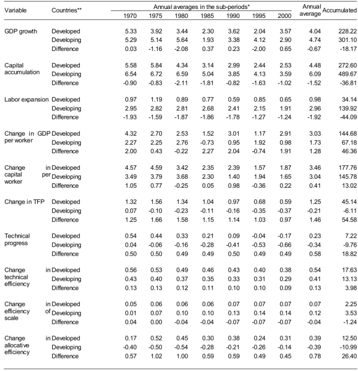
We will now take a closer look at the differences in economic growth patterns of developed and developing nations. Table 4 and Graph 3 bring data on GDP growth and the sources of growth for two groups of countries10. Table 4 displays annual averages (for each five-year period and for the whole 30 five-year period). For economic growth and each of its sources we computed the difference between the rate of change calculated for developed nations and that calculated for developing countries. The same was done for the productivity components.

10

(26)

Table 4. Sources of economic growth per group of countries and periods – % change

Annual averages in the sub-periods* Variable Countries**

1970 1975 1980 1985 1990 1995 2000 Annual

average Accumulated

Developed 5.33 3.92 3.44 2.30 3.62 2.04 3.57 4.04 228.22 Developing 5.29 5.14 5.64 1.93 3.38 4.12 2.90 4.74 301.10 GDP growth

Difference 0.03 -1.16 -2.08 0.37 0.23 -2.00 0.65 -0.67 -18.17

Developed 5.58 5.84 4.34 3.14 2.99 2.44 2.53 4.48 272.60 Developing 6.54 6.72 6.59 5.04 3.85 4.13 3.59 6.09 489.67 Capital

accumulation

Difference -0.90 -0.83 -2.11 -1.81 -0.82 -1.63 -1.02 -1.52 -36.81

Developed 0.97 1.19 0.89 0.77 0.59 0.85 0.65 0.98 34.14 Developing 2.95 2.82 2.81 2.68 2.41 2.15 1.91 2.96 139.92 Labor expansion

Difference -1.93 -1.59 -1.87 -1.86 -1.78 -1.27 -1.24 -1.92 -44.09

Developed 4.32 2.70 2.53 1.52 3.01 1.17 2.91 3.03 144.68 Developing 2.27 2.25 2.76 -0.73 0.95 1.92 0.98 1.73 67.18 Change in GDP

per worker

Difference 2.00 0.43 -0.22 2.27 2.04 -0.74 1.91 1.28 46.36

Developed 4.57 4.59 3.42 2.35 2.39 1.57 1.87 3.46 177.76 Developing 3.49 3.79 3.68 2.30 1.40 1.94 1.65 3.04 145.78 Change in

capital per worker

Difference 1.05 0.77 -0.25 0.05 0.98 -0.36 0.22 0.41 13.02

Developed 1.32 1.56 1.34 1.04 0.97 0.68 0.59 1.25 45.14 Developing 0.07 -0.10 -0.23 -0.11 -0.16 -0.35 -0.37 -0.21 -6.11 Change in TFP

Difference 1.25 1.66 1.58 1.15 1.14 1.03 0.97 1.46 54.58

Developed 0.54 0.44 0.33 0.21 0.09 -0.04 -0.17 0.23 7.22 Developing 0.04 -0.06 -0.16 -0.28 -0.41 -0.53 -0.66 -0.34 -9.76 Technical

progress

Difference 0.50 0.50 0.49 0.49 0.50 0.49 0.49 0.58 18.82

technical efficiency

Difference 0.13 0.13 0.12 0.11 0.10 0.10 0.09 0.13 3.98

efficiency of scale

Difference 0.04 0.00 -0.04 -0.04 -0.07 -0.07 -0.07 -0.04 -1.24

Developed 0.17 0.52 0.45 0.30 0.38 0.24 0.31 0.39 12.50 Developing -0.40 -0.50 -0.54 -0.28 -0.21 -0.26 -0.14 -0.39 -10.99 Change in

allocative efficiency

Difference 0.57 1.02 1.00 0.59 0.59 0.49 0.45 0.78 26.40

* The years represent the final point of each period, e.g., 1970 refers to the five-year period from 1966 to 1970, 1975 refers to the

five-year period from 1971 to 1975, and so on. ** The values in this table were calculated by taking the simple average of the rates of change

during the sub-periods for the countries comprising each group. The accumulated affect is computed by compounding the rates and discounting

(27)

We see that developing nations grew more than developed ones (18.2%). This happened because both capital accumulation as well as labor expansion were larger in developing countries. However, the growth of GDP per worker was greater in developed countries, which can be attributed basically to two factors: (i) the difference between the growth rates of capital and labor was greater in developed nations, thus providing higher growth of capital per worker; (ii) the change in TFP in developed nations was considerably higher than in developing ones (yet it should be said that in the second group this change pushed down GDP’s growth). The differences between the two groups in regard to growth of capital per worker are well below the differences in TFP growth. This suggests that productivity plays a role of great importance in the development of nations, better yet, that it might explain a significant part of the differences in GDP per capita growth between rich and poor countries.

If we take a look at the relative importance of the components of productivity, we see that developed nations have some advantages, even if minor, in regard to technical efficiency. On the other hand, we also see that this difference is in part offset by positive scale effects enjoyed by developing countries. Judging by the magnitude of the differences between the groups of countries regarding the pace of technical progress and the evolution of allocative efficiency, we are able to conclude that these two components explain most of the differences in productivity existing between the two groups. While developed nations enjoyed technical progress of 7.2% in the 30 years analyzed here, developing countries in fact suffered a 9.8% drop in that component, a gap that adds up to 18.8%. We also notice that rich countries accumulated sizable 12.5% in allocative efficiency improvement, at the same time that in poor countries this variable fell 11%. Here we have an accumulated difference of 26.4% in this component, which places this figure at the forefront in explaining the differences in productivity among the two groups of countries, and consequently the differences in the rates of output growth.

(28)

(29)

Graph 3. Sources of growth per group of countries 2000 1995 1990 1985 1980 1975 1970 C ontr ibuti

on of fac

tor ac cu mul a tion ,25 ,20 ,15 ,10 ,05 0,00 -,05 -,10

1970 1975 1980 1985 1990 1995 2000

C

ontr

ibuti

on of T

F P ,25 ,20 ,15 ,10 ,05 0,00 -,05 -,10 2000 1995 1990 1985 1980 1975 1970 T ec hni cal pr ogr es s ,08 ,06 ,04 ,02 0,00 -,02 -,04 2000 1995 1990 1985 1980 1975 1970 T e chni ca l effi ci enc y ,08 ,06 ,04 ,02 0,00 -,02 -,04 2000 1995 1990 1985 1980 1975 1970 S cal e effi ci enc y ,08 ,06 ,04 ,02 0,00 -,02 -,04 2000 1995 1990 1985 1980 1975 1970 A llo ca tiv e effi ci enc y ,08 ,06 ,04 ,02 0,00 -,02 -,04

(30)

Graph 4 reinforces this notion. It illustrates the relation between the governance index developed by Kaufmann, Kraay and Zoido-Lobatón (1999), and the average annual change in allocative efficiency for the 36 economies, from 1970 to 2000. As expected, the economies with better governance enjoyed less distortions and consequently greater allocative gains. The other graph shows the relation, for 33 of these 36 economies, from 1970 to 2000, between allocative efficiency and the degree of liberalization of financial flows, according to the measure suggested by Santana (2004). Also in this case, where we see five-year changes in these two measures, the elimination of distortions brought by barriers to the flow of capital seem to benefit the growth of allocative efficiency.

Graph 4 Governance, financial liberalization and allocative efficiency

Governance Index 1,2 1,0 ,8 ,6 ,4 ,2 A llo ca ti ve e ff ici e n cy ,04 ,02 0,00 -,02 -,04 -,06 -,08 VEN USA TUR TTO THA SWE PRT PER NZL NOR NLD MEX KOR KEN JPN JOR JAM ITA ISLIRL GRC GBR FRA FIN ESP DNK CRI COL CHL CHE CAN BRA BOL BEL AUT AUS

Capital account openness

1,00 ,80 ,60 ,40 ,20 0,00 A llo ca ti ve e ffi ci e n c y ,10 ,05 0,00 -,05 -,10

Source: Kaufmann, Kraay and Zoido-Lobatón (1999), Santana (2004) and own data.

7

7 C

C

o

n

c

l

u

d

i

n

g

r

e

m

a

r

k

s

Two excerpts from contemporary remarks made by Robert Solow reveal that much remains to be clarified regarding the determinants of economic growth and their relative importance:

“…Bits of experience and conversation have suggested to me that it may be a

mistake to think of R&D as the only ultimate source of growth in total factor

(31)

lot of productivity improvement that originates in people and processes that are not

usually connected with R&D. Some of it comes from the shop floor, from the ideas of

experienced and observant production workers. This should probably be connected with

Arrow’s “learning by doing” or with the Japanese slogan about “continuous

improvement.” There is another part that seems to originate in management practices –

in design, in the choice of product mixes, even in marketing. Notice that this is not just

straightforward enhancement of productive efficiency. All this talk about value creation

may be more than a buzzword; it may even be important. We need to understand much

more about how these kinds of values get reflected in measured real output, and whether

they can be usefully analyzed by our methods.”

Solow (2001a)

“…the nontechnological sources of differences in TFP may be more important

than the technological ones. Indeed they may control the technological ones, especially

in developing countries.”

Solow (2001b)

The results presented in the previous sections readily provide information to clarify the apparent contradiction between these two statements. Even if restricted to a relatively small sample of countries, the results presented in Table 4 reveal that, in fact, for developed nations technical progress and technical efficiency changes are responsible for the larger part of TFP change accumulated in the last 30 years: of the 45.1 percentage points increase in TFP, 26.1 can be attributed to the joint effect of these two components (i.e., around 58% of all change). Yet for developing nations, for which TFP had a 6.1 percentage points decrease during the same period, the component that contributed the most to this result is allocative efficiency change, which reduced productivity in nearly 11 percentage points. Together, technical progress and changes in allocative efficiency contributed with a small accumulated growth of 2.1 percentage points. This technological performance is unsatisfactory in large part due to relatively small investments made by poor nations in R&D.

(32)

income per worker and TFP) - about 60% of these differences. The pattern of technical progress is behind the other 40% of the gap. These facts point out that economic policies that directly affect factor allocation are extremely relevant in explaining the differences in the growth performance between developed and developing countries.

Regarding the changes in productivity associated with technological diffusion and waste reduction, the results of the article allow us to identify the importance of the increase in technical efficiency estimated by the stochastic frontier model, which contributes both to the growth of developed nations as well as developing ones. This perception seems to be in part shared by Robert Solow. The examples given by Solow are typical of what the production frontier literature calls efficiency improvement, both technical and allocative. Since he does not consider the explicit possibility of inefficiency, Solow seems to consider these phenomena some sort of innovation, yet not related to R&D expenses (design, marketing, etc.). However, we clearly see that he feels that technical progress leveraged by R&D spending is not the only driver of productivity.

Recently, Easterly & Levine (2001) added fuel to the existing controversy among the scholars espousing the “sources of economic growth”, on the relative importance of factor accumulation and productivity. The underlying objective of these authors is to demonstrate that, unlike what is preached by the “Neoclassical Revival”, the focus of investigation of economic growth should be productivity and its determinants11. The authors list five stylized facts regarding economic growth to underpin their idea. Some of their findings are corroborated by the results of this study, but others are not.

The first stylized fact presented by these authors states that differences in TFP growth explain the differences in per-capita income and per-capita income growth rates among the various countries. Although factor accumulation may be important to trigger growth and be responsible for a sizable share of this growth in a number of countries, it is not able to explain the

11_{Klenow & Rodriguez-Clare (1997) use this terminology created by Alwyn Young to qualify a body of}

(33)

differences in level of income or in rates of income change among nations. In relation to this fact, it should be pointed out, first of all, that the great importance of capital accumulation in the countries’ growth rate also appears in the results for the reduced 36-country sample. In fact, we find that 80% of the growth would be attributable to the accumulation of capital and labor, and only the 20% remaining would come from productivity gains. The results vary when we calculate separately the average for the group of 24 developed countries (factor accumulation is lower, close to 63% of the growth) and for the group of 12 developing nations (contribution to productivity is negative and therefore the factor accumulation is behind all the economic growth).

If our reference is output per worker, the importance of capital accumulation remains high. With some additional calculations based on the numbers listed in Table 4, we conclude that on average 62.1% of the GDP growth is due to capital accumulation. Klenow & Rodriguez-Clare (1997) reach a similar result for a sample of 98 countries: on average 70% of economic growth is the result of physical and human capital accumulation. The comparison is obviously limited, because human capital is not considered in this study and because the samples are different. Nonetheless, the reduced sample used in this article contains 24 of the 30 OECD members, while the sample used by Klenow & Rodriguez-Clare (1997) contains all of them. Consequently, we can conclude that most of the nations that differentiate the two samples are developing economies, which generally have a higher share of capital in income. Thus, the inclusion of these countries would tend to raise the participation of factors in the growth of GDP per worker (above 62.1%), bringing the results of the two samples closer to each other.

(34)

The divergence between developed and developing nations was one of the results found using the empirical model applied in this study. Moreover, it is clear that the differences in the rates of productivity change are behind all the differences in the rates of growth of GDP per worker (the accumulation of factors contributed towards reducing such differences). Note that this result was obtained within the traditional framework of an aggregated production function with diminishing returns. It was not necessary to incorporate in the analysis a new sector (a knowledge production sector presenting increasing returns).

The third stylized factor in the Easterly & Levine (2001) list suggests that the accumulation of factors is persistent, at the same time that economic growth is not. Considering that changes in the rate of growth depend both on changes in factor accumulation as well as on changes in productivity, the validity of this stylized fact implies that TFP cannot be persistent. A consequence of this is that productivity measures would necessarily have a volatile behavior. This could be avoided if production data to be explained reflected the potential, rather than the actual product.

Robert Solow (Solow, 2001a) says that growth theory is a theory of the evolution of potential product. This is justified by the fact that the countries’ growth paths do not resemble at all the concept of steady state. In economies where agriculture has a considerable weight, sudden weather changes or pests can bias the traditional TFP measure. Consequently, either we work with potential output as a dependent variable or we add explanatory variables that controls for weather changes or pests. Demand fluctuations are another source of deviation of output from its balanced growth path. If we return to Graph 3 and examine the evolution of productivity change, we see that it has an absolutely “serene” behavior. Here probably lies the greatest contribution of the approach combining stochastic production frontier estimation and the Bauer-Kumbhakar decomposition: it allows us to separate the effects of random shocks from the other TFP components. All the other TFP components have a clear trend, with little fluctuation, except perhaps for allocative efficiency, which responds to policies.

(35)

to evaluate if the assumptions of a normal truncated distribution for the technical efficiency component and of normal distribution with zero mean for the random component describe well the behavior of the observed data. The analysis of the residuals shows that the presumption of normal distribution with zero mean seems to suit the data well.

The fourth stylized fact points out that production factors tend to flow towards the same direction and as a consequence economic activity is quite concentrated. This is valid not only among countries but also within them (regions, states and cities). If there were no productivity differences, the trend would be exactly the opposite, i.e., that of an even distribution of factors among the various countries, because of the presence of decreasing returns. Differences in policies could explain factor accumulation (regulation, tax structure, legal systems, public education, etc.). However, usually these policies have a nationwide scope and would not be helpful in explaining concentration within the nations. Easterly & Levine (2001) do not provide a single explanation for this phenomenon and argue that such stylized fact is consistent with existing explanations in terms of poverty traps, intra-group factors or geographical externalities, and is also consistent with explanations based on differences of productivity caused by technological differences.

The results of this article have shown that developing nations accumulate production factors at a much faster pace than that of developed nations and for this reason also grow faster. The model used presents a measure of scale effects for the sample countries that is intuitive but not fully consistent with the notion of concentration of economic activity, because there are a number of developing economies that presented increasing returns to scale (India, Indonesia, Brazil and Mexico, to name a few). However the magnitude of the scale effects estimated is not up to the task of explaining the fourth stylized fact identified by Easterly & Levine (2001).

(36)

efficiency. As seen, the results presented in this study show the great importance of allocative efficiency change in productivity change, and consequently in growth rate differences.

(37)

A

p

e

n

d

i

x

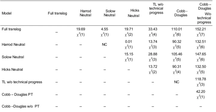
The likelihood ratio statistic is given byλ=−2[LˆR −LˆNR], where Lˆ e R LˆNR are,

respectively, the estimated log-likelihood of the described model and of the non-restrict model. The table below summarizes the tests performed. The null hypothesis under question is always that the model identified in the matrix column is nested in the model of the matrix line. The LR statistic has a χ2 (DF) type distribution, where DF shows the difference in the degrees of freedom among the various models. If the value expressed in the cell of the statistics matrix is greater than the critical value, then the null hypothesis cannot be rejected, otherwise it can be rejected.

Table A.1 Likelihood ratio tests

Model Full translog _NeutralHarrod _NeutralSolow Hicks Neutral

TL w/o technical

progress Cobb -Douglas Cobb – Douglas W/o technical progress Full translog

-- 19.69 _χ2

(1) 4.55 χ2 (1) 19.71 χ2 (2) 33.43 χ2 (4) 110.01 χ2 (6) 152.21 χ2 (7)

Harrod Neutral -- -- NC _χ0.01 2

(1) 13.74 χ2 (3) 90.32 χ2 (5) 132.51 χ2 (6)

Solow Neutral -- -- -- 15.15 _χ2

(1) 28.88 χ2 (3) 105.46 χ2 (5) 147.65 χ2 (6)

Hicks Neutral -- -- -- -- 13.72 _χ2

(2) 90.31 χ2 (4) 132.50 χ2 (5)