www.biogeosciences.net/14/631/2017/ doi:10.5194/bg-14-631-2017
© Author(s) 2017. CC Attribution 3.0 License.
Quantifying nutrient fluxes with a new hyporheic passive
flux meter (HPFM)
Julia Vanessa Kunz1, Michael D. Annable2, Jaehyun Cho2, Wolf von Tümpling1, Kirk Hatfield2, Suresh Rao3, Dietrich Borchardt1, and Michael Rode1
1Helmholtz Centre for Environmental Research UFZ, Magdeburg, Germany 2University of Florida, Gainesville, Florida, USA
3Purdue University, Lafayette, Indiana, USA
Correspondence to:Julia Vanessa Kunz (vanessa.kunz@ufz.de) Received: 11 August 2016 – Discussion started: 19 August 2016
Revised: 20 January 2017 – Accepted: 23 January 2017 – Published: 9 February 2017
Abstract. The hyporheic zone is a hotspot of biogeochem-ical turnover and nutrient removal in running waters. How-ever, nutrient fluxes through the hyporheic zone are highly variable in time and locally heterogeneous. Resulting from the lack of adequate methodologies to obtain representa-tive long-term measurements, our quantitarepresenta-tive knowledge on transport and turnover in this important transition zone is still limited.
In groundwater systems passive flux meters, devices which simultaneously detect horizontal water and solute flow through a screen well in the subsurface, are valuable tools for measuring fluxes of target solutes and water through those ecosystems. Their functioning is based on accumulation of target substances on a sorbent and concurrent displacement of a resident tracer which is previously loaded on the sorbent. Here we evaluate the applicability of this methodology for investigating water and nutrient fluxes in hyporheic zones. Based on laboratory experiments we developed hyporheic passive flux meters (HPFMs) with a length of 50 cm which were separated in 5–7 segments allowing for vertical resolu-tion of horizontal nutrient and water transport. The HPFMs were tested in a 7 day field campaign including simultaneous measurements of oxygen and temperature profiles and man-ual sampling of pore water. The results highlighted the ad-vantages of the novel method: with HPFMs, cumulative val-ues for the average N and P flux during the complete deploy-ment time could be captured. Thereby the two major deficits of existing methods are overcome: first, flux rates are mea-sured within one device instead of being calculated from sep-arate measurements of water flow and pore-water
concentra-tions; second, time-integrated measurements are insensitive to short-term fluctuations and therefore deliver more repre-sentable values for overall hyporheic nutrient fluxes at the sampling site than snapshots from grab sampling. A remain-ing limitation to the HPFM is the potential susceptibility to biofilm growth on the resin, an issue which was not con-sidered in previous passive flux meter applications. Poten-tial techniques to inhibit biofouling are discussed based on the results of the presented work. Finally, we exemplarily demonstrate how HPFM measurements can be used to ex-plore hyporheic nutrient dynamics, specifically nitrate uptake rates, based on the measurements from our field test. Being low in costs and labour effective, many flux meters can be installed in order to capture larger areas of river beds. This novel technique has therefore the potential to deliver quanti-tative data which are required to answer unsolved questions about transport and turnover of nutrients in hyporheic zones.
1 Introduction
for example retain up to 38 % of nitrate (NO−3)and 48 % of soluble reactive phosphate (SRP) inputs (Mortensen et al., 2016). The hyporheic zone, the subsurface region of streams and rivers that exchanges water, solutes and particles with the surface (Valett et al., 1993) and may mix streamwater during the transport through the sediments with underlying ground-water (Triska et al., 1989; Fleckenstein et al., 2010; Trauth et al., 2014), is one key compartment for in-stream nutrient cycling (Fischer et al., 2005; Zarnetske et al., 2011b; Basu et al., 2011; Stewart et al., 2011). For instance, denitrifica-tion, the anaerobic reduction of NO−3 to gaseous N2and in
most river systems the dominant dissimilatory process which removes N out of the system (Laursen and Seitzinger, 2002; Bernot and Dodds, 2005; Lansdown et al., 2012; Kunz et al., 2017), often exclusively happens at “reactive sites” in the hy-porheic zone (Duff and Triska, 1990; Rode et al., 2015). In addition to biological nutrient uptake, intermediate physical storage in the hyporheic zone disperses the propagation of pollutant and nutrient spikes which could be harmful for re-ceiving water bodies (Runkel, 2007; Brookshire et al., 2009; Covino et al., 2010; Findlay et al., 2011). For those reasons, it is of interest to quantify the amount of nutrients actually reaching the reactive sites in the subsurface collateral to the processes they undergo there (Seitzinger et al., 2006; Zar-netske et al., 2012). Transport rates of water and nutrients from the surface to the subsurface could be attributed to wa-ter level, sediment properties and various other hydrologi-cal, biologihydrologi-cal, chemical and physical factors (Böhlke et al., 2009; Boano et al., 2014; Trauth et al., 2015). The complex interactions between these influencing factors and the tempo-ral variability and local heterogeneity of hyporheic processes often cause high uncertainties in quantitative models. How-ever, due to methodological restrictions, experimental inves-tigations of nutrient dynamics in the hyporheic zone are rare and commonly exclusively of qualitative nature (Mulholland et al., 1997; Grant et al., 2014).
Attempts to quantify hyporheic nutrient processing rates have primarily been based on benthic chamber and incuba-tion experiments (Findlay et al., 2011; Kessler et al., 2012). Those laboratory (mesocosm and flume) experiments can es-timate the denitrification potential of the substrates, usually via denitrification enzyme assays. However, the realised den-itrification rates depend equally on environmental and hydro-logical conditions rather than on substrate type or denitrifica-tion potential alone (Findlay et al., 2011). Thus, owing to the high variability and complexity of natural systems, hyporheic transport of nutrients cannot satisfactorily be mimicked in ar-tificial set-ups (Cook et al., 2006; Grant et al., 2014).
Direct in-stream measurements of nutrient dynamics based on whole-stream tracer injections, mass balances (McKnight et al., 2004; Böhlke et al., 2009) and more re-cently high-resolution time series from automated sensors (Pellerin et al., 2009; Hensley et al., 2014; Rode et al., 2016a, b) can be used for determining general uptake rates on the reach scale, but do not allow to identify the reaction sites
(hyporheic versus in channel or algal canopies) or specific local uptake processes (Ensign and Doyle, 2006; Ruehl et al., 2007). Further, in-stream measurements exclusively ac-count for water which is re-infiltrating into the main stem af-ter passage through the hyporheic zone. Under loosing con-ditions, where most of the nutrient-influx is flowing towards the groundwater, processing rates in the subsurface cannot be observed in the surface water. Likewise, if groundwater is contributing significantly to surface water chemistry, surface water mass balances do not characterise nutrient cycling in the hyporheic zone realistically (Trauth et al., 2014).
Conclusively, in situ assessments of hyporheic nutrient fluxes are indispensable. Hyporheic nutrient fluxes are com-monly calculated from separate measurements of infiltration rates and pore-water concentrations (Kalbus et al., 2006; Ingendahl et al., 2009). The exchange of water between the surface and subsurface is traditionally derived from hy-draulic head differences or tracer injections (Fleckenstein et al., 2010; USEP, 2013). Time series of high-resolution ver-tical temperature profiles have efficiently been used to de-rive vertical Darcy velocity (qy) (m d−1)in the streambed.
While measurements of vertical Darcy velocities are a valu-able asset, primarily horizontal fluxes are needed to assess hyporheic transport and residence time (Binley et al., 2013; Munz et al., 2016). Active heat-pulse tracing enables highly resolved in situ measurements of direction and velocity of hyporheic flow (Lewandowski et al., 2011; Angermann et al., 2012). These methods are profitable in shallow sediments (max. 15–20 cm) and rivers with fine sediments, but may not be implementable in streams with coarser sediments.
techniques for measuring pore-water concentrations exclu-sively capture the concentration at the sampling time, which may not reflect the overall conditions at the sampling loca-tion. New, affordable and efficient methods for the long-term measurement of nutrient fluxes through the hyporheic zone are therefore required to validate and improve models (Boyer et al., 2006; Wagenschein and Rode, 2008; Alexander et al., 2009) and to determine the site-specific extent of nutrient processing in the hyporheic zone (Fischer et al., 2009).
In groundwater studies, passive flux meters (PFMs) have successfully been used to quantify fluxes of contaminants (Hatfield et al., 2004; Annable et al., 2005; Verreydt et al., 2013) through screened groundwater monitoring wells, inte-grating time spans ranging from days to weeks. PFMs consist of a cylindrical, screened PVC casing filled with activated carbon (AC) as a porous sorbent. As long as the PFM is re-siding in the monitoring well, dissolved contaminants in the groundwater flowing passively through the meter are retained on the AC. Furthermore, the AC is preloaded with water-soluble resident tracers. The horizontal water flux through the screened media can then be determined from the dis-placement of these resident tracers, while simultaneously the contaminant flux is quantified based on the solute mass cap-tured on the AC. First bench-scale and column experiments for PO−4 have been conducted in the laboratory (Cho et al., 2007). As AC did not prove efficient in capturing nutrients, an anion-absorbing resin, a granular matrix originally man-ufactured for purification processes, was used as sorbent for PO−4 instead. In theory, the PFM principle should be extend-able to other nutrients or other environments. For example, development of sediment bed passive flux meters (SBPFMs) for the measurement of vertical contaminant seepage has been initiated (Layton, 2015). However, specific tests for NO−3 as well as assessments under the complexities associ-ated with hyporheic zone processes have not been conducted yet.
In this study we evaluate the applicability of PFMs for the measurement of horizontal nutrient fluxes in hyporheic zones, focusing on NO−3. We hypothesised that, while the principal concept of PFM can be maintained, several adap-tations will still be necessary: most importantly, a suitable sorbent for NO−3 as target nutrient is required. The market of anion-absorbing resins is large and offers a wide range of products with varying characteristics (Annable et al., 2005; Clark et al., 2005). Various criteria, like possible interfer-ence of resin compounds with the resident tracer analysis or pre-existing background nutrient loads on the resin, have to be considered. As experience on resin behaviour under field conditions is so far rare, we also expected unforeseen associated challenges, including for example biofouling of resin and/or nutrients. Additionally, a new deployment and retrieval procedure had to be developed. Existing ground-water PFMs have been installed into land-based wells. In hyporheic studies, underwater installation requires a tech-nique which impedes contamination with surface water.
Cor-rections for convergence and divergence of flowlines into or around the flux meter have been established in earlier studies (Klammler et al., 2007). However, accounting for an imper-meable outer casing of a flux meter is much more compli-cated and requires additional factors which have to be deter-mined experimentally for each specific application (Hatfield et al., 2004; Klammler et al., 2007; Annable et al., 2005). We therefore intended to deploy the PFM in a way that allows direct contact with the surrounding sediments and minimal manipulation of the natural flow pattern.
Considering these requirements, we developed a modifi-cation of the PFM for the applimodifi-cation in the hyporheic zone (hyporheic passive flux meter, HPFM). Based on the results from laboratory analysis and a first field test in a nutrient-rich 3rd-order stream (Holtemme, Germany), we demon-strate prospects and remaining limitations for hyporheic nu-trient studies with HPFMs.
2 Methods
2.1 Construction and materials
The HPFMs consisted of a nylon mesh which was filled with a mixture of a macroporous anion exchange resin as a nu-trient absorber and alcohol tracer loaded activated carbon (AC) for the water flow quantification. In the present study HPFMs were constructed 50 cm long and 5 cm in diameter. A stainless steel rod in the middle assured the stability of the device (Fig. 1). To measure vertical profiles of horizontal fluxes of both nutrient and water in the hyporheic zone, the HPFM was divided into several segments using rubber wash-ers. Steel tube clamps were used to attach the nylon mesh to the steel rod placed in the centre of the HPFM. The nylon mesh was purchased from Hydro-Bios (Hydro-Bios Appa-ratebau GmbH, Kiel-Holtenau, Germany) and is available in a wide range of mesh size and thicknesses. We used a mesh size of 0.3 mm. In general, meshes should be as wide as pos-sible because very fine mesh may act as a barrier to water flow limiting infiltration of water and solutes into the HPFM (Ward et al., 2011). However, the mesh should be smaller than the finest sediments, AC or resin granules. As final step, a rope was connected to the tube clamp on the upper end of the HPFM in order to facilitate retrieval.
2.2 Selection and characterisation of resin
The nutrient sorbent had to meet the following criteria: 1. have a high loading capacity for NO−3 , PO−4 and
com-peting anions;
Figure 1.Photograph of an HPFM with alternating segments before deployment (left), schematic profile of a deployed HPFM (middle) and schematic steps of HPFM functioning (right): (1) directly after installation, tracer resides on activated carbon (AC), (2) infiltrating water washes out the tracer, nutrients enter the HPFM and are absorbed on the resin, (3) after retrieval nutrients are fixed on the resin, tracer concentration is diluted.
A pre-selection for anion-absorbing resins which were free of organic compounds was made based on information provided by the manufacturers (Purolite®, Lewatit®, Dowex®). 2.2.1 Nutrient background
Nutrient background on the resins was determined by ex-tracting and analysing NO−3 and PO−4 from each resin (n= 3). Therefore 30 mL of 2M KCl was added to 5 g of each pure resin and rotated for 24 h. The solution was then analysed on a Segmented Flow Analyser Photometer (DR 5000, Hach Lange) for NO−3 at 540 nm (detection limit 0.042 mg NO−3-N L−1) and for SRP at 880 nm (detection
limit 0.003 mg P L−1). In order to estimate the effect of back-ground concentrations on final results in the actual field ap-plication of HPFM, the extractable background concentra-tions were then converted to nutrient fluxes using a Darcy flux of qx=4 m d−1, an estimate based on hyporheic flow
velocities which were measured previously with salt tracer tests at the study site. Likewise, the expected hyporheic nu-trient flux was computed from previously examined concen-trations in pore-water samples and the Darcy flux. The only resin with nutrient background below 5 % of expected con-centrations was Purolite® A500 MB Plus (Purolite GmbH, Ratingen, Germany), which had extractable background NO−3 of 8 µg NO−3-N g−1wetted resin (±1.6 µg g−1,n=3)
and 0.08 µg PO−4-P g−1 resin (±1.7×10⁻³µg g−1, n=3). Purolite®A500 MB Plus was then considered for testing the loading capacity. The limit of quantification LQ for the nutri-ent extraction resulting from this background was calculated according to the EPA Norm 1020B (Greenberg et al., 1992) as the sum of background concentration and 10 times the standard deviation and amounted to 24 µg NO−3-N g−1resin and 0.097 µg PO−4-P g−1resin.
2.2.2 Loading capacity and biofouling
Purolite®A500 MB Plus is a macroporous anion exchanger on the basis of polyvinylbenzyl-trimethylammonium with a typical granular size of 0.88 mm diameter, an average den-sity of 685 g L−1 and an effective porosity of 63 %. The theoretical absorbing capacity is indicated in the product sheet as 1.15 eq L−1 (molar weight equivalences per litre
of resin), corresponding to 71.3 g NO−3-N L−1. Assuming
hyporheic flow velocities ofqx=4 m d−1 and a
concentra-tion of 10 mg NO−3-N L−1, the volume of one HPFM could adsorb NO−3 for 89 days. However, if multiple anions are present, real loading capacities for NO−3 are expectedly lower.
For the determination of a realistic loading capacity, three 5 cm diameter columns were filled to a height of 5 cm with wetted Purolite® A500 MB Plus resin, placed in a vertical position and infiltrated with water collected from the study reach. The columns were covered with tin foil to keep them dark and ensure stable temperature. A constant supernatant of 1 cm was kept on all three columns to ensure uniform infiltration at the surface of the column. Water was contin-uously pumped (peristaltic pump, ISMATEC® BVP Stan-dard, ISM444) through the columns from top to bottom for 22 days at a speed of 20 mL h−1, which also equals the
ex-pected Darcy velocity ofqx=4 m d−1. River water was
sup-plied from a 22 L HDPE canister (Rotilabo®EPK0.1). SRP and NO−3 concentrations in this reservoir were revised daily. The draining water at the bottom outlet of the columns was sampled twice a day and analysed for SRP and NO−3.
the loading capacity could be monitored. After the experi-ment we coloured samples (n=3) of resin granules from the columns with SybrGreen (C32H37N4S+)on nucleic acid and
examined them under a confocal laser scanning microscope to depict the degree of bacterial fouling on the granular sur-face.
2.3 Preparation of activated carbon with alcohol tracers
As designed for the groundwater PFMs, silver impregnated activated carbon (AC) was used as sorbent for the resident alcohol tracers. The same AC as in previous PFM appli-cations (Annable et al., 2005) was used for the HPFM in this study and was provided by the University of Florida, Gainesville. The AC had a bulk density of 550 g L−1, a grain size ranging from 0.42 to 1.68 mm and a hydraulic conduc-tivityk=300 m d−1.
Since the magnitude of water flow through the flux meter is unknown a priori, multiple resident tracers with a wide range of tracer elution rates were needed. The retardation factor of a substanceRdis a measure for the rate of elution
of the substance from a particular carrier. Alcohols offer a wide range of retardation factors and can easily be mixed and sorbed to the AC (Hatfield et al., 2004; Cho et al., 2007). By choosing the same manufacturer for the AC and the same alcohol mixture as used in the above-mentioned stud-ies, we could rely on physical and chemical characterisations and calculated Rd for alcohol partitioning behaviour which
have been established by Hatfield et al. (2004), Annable et al. (2005) and Cho et al. (2007) (Table 1).
An alcohol tracer mixture for approximately 10 HPFMs was prepared by combining 100 mL of methanol, 100 mL of ethanol, 200 mL of isopropanol (IPA), 200 mL oftert-butanol (TBA) and 66 mL of 2,4-dimethyl-3-pentanol (2,4 DMP).
In order to prepare the resident alcohol tracers on the AC, the AC was soaked in an aqueous solution containing the res-ident alcohol tracers. A standard ratio of 13 mL tracer mix-ture was added to 1 L of water in a Teflon sealed container and was then shaken by an automated shaker over a period of several hours. Subsequently, 1.5 L of dry activated carbon was added to the aqueous tracer solution and rotated for 12 h to homogenise the AC tracer mixture. After mixing, the su-pernatant water was discarded and the AC tracer mixture was stored in a sealed container and refrigerated, preventing the evaporation of the alcohol tracers.
Similarly to the resins, the AC was tested for background nutrients by extraction with 30 mL KCl per 5 g AC.
The activated carbon contained 0.01 mg PO−4-P g−1AC (±7.5×10⁻⁴mg g−1, n=3) and 0.08 mg NO−
3-N g
−1AC
(±5×10⁻³mg g−1,n=3), which amounts to 75 % of the expected concentration for NO−3 and 320 % for PO−4. To investigate whether the AC could be cleaned by washing, we repeatedly treated AC samples with distilled water or KCl as depicted in the extraction description above.
Nutri-ents did not leach off under water treatment and neither did KCl treatment satisfactorily reduce extractable background concentration on the AC. After the third washing of AC with KCl, 0.02 mg PO−4-P (±3.3×10⁻⁴mg g−1,n=3) and 0.04 mg NO−3-N (±2.3×10⁻³mg g−1,n=3) could still be extracted per g AC. Further, it was unclear to which degree replacing absorbed nutrients by KCl would alter the alcohol tracer retardation and extraction on the AC. For those rea-sons, we decided to keep the nutrient-absorbing resin sepa-rated from the AC. As AC did not release background nutri-ents under water treatment, water flowing first through AC and afterwards resin layers was not considered problematic. 2.4 Deployment and retrieval procedure
HPFMs were built, stored dry and transported in 70 cm long standard polyethylene (PET) tubes (58×5.3 SDR 11) purchased from a local hardware store (Handelshof Bitter-feld GmbH, BitterBitter-feld, Germany). To avoid resident alcohol tracer loss, the transport tubes with the HPFMs were sealed with rubber caps and cooled during storage and transport. In the field, prior to installation, the HPFMs were transferred to a stainless steel tube, 5.3 cm inner diameter with a loose steel drive point tip on the lower end. The diameter of the steel tube for installation tightly fitted with the rubber wash-ers at the top and bottom end of the HPFM, so that vertical water flow through tube and HPFM during installation was inhibited. The steel casing and HPFM were driven into the river bed using a 2 kg hammer until the upper end of the HPFM was at the same level as the surface–subsurface in-terface. The metal casing was retrieved while the HPFM was held in place using a steel rod.
After 7 days of exposure, the HPFMs were retrieved by holding the transport tube in place and quickly drawing the HPFM into the tube using the rope fixed to the upper end of the HPFM. The required length of the transport tube, steel drive casing and retrieval rope was determined by the depth of the water level in the stream.
After retrieval, the HPFMs were transported to the labora-tory.
2.5 Analysis and data treatment
In the laboratory, the retrieved HPFMs were instantly (after maximal 12 h) sampled for analysis. Therefore one segment after the other was cut open and the sorbent was segment-wise recovered, homogenised and a subsample transferred to 40 mL glass vials. The subsamples from resin segments were then analysed for nutrient content, the subsamples from AC segments were analysed for the remaining alcohol tracers as described in the following paragraphs.
2.5.1 Water flux
Table 1.Resident tracers per litre of aqueous solution and their partitioning characteristics. Retardation factors (Rd) for the specific set of tracers and AC used in this study had previously been determined by Cho et al. (2007).
Resident tracers Aqueous concentration (g L−1) Rd
Methanol 1.2 4.9
Ethanol 1.2 20
Isopropyl alcohol (IPA) 2.3 109
tert-Butyl alcohol (TBA) 2.3 309
2,4-Dimethyl-3-pentanol (DMP) 1.2 >1000
mixture of alcohol tracers in standard AC samples and the tracer mass remaining in the final AC samples were extracted with iso-butyl alcohol (IBA). About 10 g of AC samples were transferred into pre-weighed 40 mL vials containing 20 mL IBA. Vials were rotated on a Glas-Col Rotator, set at 20 % rotation speed, for 24 h. Then, subsamples were collected in 2 mL GC vials for alcohol tracer analysis. The samples were analysed with a GC-FID (Perkin Elmer Autosystem) (Cho et al., 2007).
The relationship between time-averaged specific horizon-tal dischargeqx(m s−1)through the device and tracer elution
is given by (Hatfield et al., 2004):
qx=
1.67rθ (1−MR)Rd
t , (1)
wherer(m) is the radius of the HPFM,θ is the volumetric water content in the HPFM (m3m−3),M
R(–) is the relative
mass of tracer remaining in the HPFM sorbent, t (s) is the sampling duration andRd(–) is the retardation factor of the
resident tracer on the sorbent. 2.5.2 Nutrient fluxJN
NO−3 and PO−4 were extracted and analysed in the laboratory at UFZ in Magdeburg, Germany, similarly to the analysis of background concentrations on the resin: subsamples of 5 g resin were treated with 30 mL of 2 M KCl each and rotated for 24 h for extraction. The solution was then analysed as described above.
The time-averaged advective horizontal nutrient flux JN
(mg m2d−1)can be calculated using the following relation-ship (Hatfield et al., 2004):
JN= qxMN
2αrLt, (2)
whereMN(kg) is the mass of nutrient adsorbed,L(m) is the
length of the vertical thickness of the segment andα(–) is a factor ranging from 0 to 2 that characterises the convergence (α >1)or divergence (α <1)of flow around the HPFM. If, like in the case presented here, the hydraulic conductivity of the HPFM sorbent (resin or AC) is much higher than that of the surrounding medium and the HPFM is in direct con-tact with the sediments (i.e. in absence of an impermeable
outer casing or well wall),αcan be estimated after Strack and Haitjema (1981):
α= 2
1+ 1
KD
!
, (3)
where KD=kDk0−1 is the dimensionless ratio of the
uni-form hydraulic conductivity of the HPFM sorptive matrixkD
(L T−1)to the uniform local hydraulic conductivity of the
surrounding sediment k0 (L T−1). For more details on the
correction factorαand applications where a solid casing is required or the permeability of the surrounding sediments is higher than of the device see Klammler et al. (2007) and Hat-field et al. (2004).
2.6 Field testing of HPFMs 2.6.1 Study site
A 30 m long stretch of the Holtemme River, a 3rd-order stream in the Bode catchment, TERENO Harz/Central German Lowland Observatory, served as study site (51◦56′30.1′′N, 11◦09′31.8′′E). The testing reach is located in the lowest part of the river, where the water chemistry is highly impacted by urban effluent and agriculture (Kamjunke et al., 2013). Long stretches have been subjected to changes in the natural river morphology by canalisation (Landesbe-trieb für Hochwasserschutz und Wasserwirtschaft Sachsen-Anhalt, 2009).
The sediments at the selected site are sandy with gravel and small cobbles. Sieving of sediment samples delivered the effective grain sized10=0.8 mm and a coefficient of
uni-formityCu=3.13. The effective porosity nef is 13 %.
Af-ter FetAf-ter (2001) the intrinsic permeability was estimated to beKi=96 m2and the hydraulic conductivityk=81 m d−1
Clay lenses are present in the deeper sediments below 35 cm. Mean discharge in the stream is 1.35 m3s−1 with
high-est peaks around 5–6 m3s−1. Discharge is continuously
Figure 2. Overview of the instrumental setup at the Holtemme for the testing phase in June 2015. R1, R2, resin-only HPFM; AC3, AC4, activated-carbon-only HPFM; L5, L6, alternating lay-ered HPFMs; MLSA, MLSB, multi-level sampler; O2 25, O2 45, subsurface oxygen logger;◦C, vertical temperature profile.
The equipment was installed for a period of 7 days from 4 to 11 June 2015 as illustrated in Fig. 2.
2.6.2 HPFM testing
Based on the laboratory results for the nutrient backgrounds and the consequent necessity to keep resin and AC separated two approaches for constructing and deploying HPFM were tested in the field.
Resin only and AC only HPFMs
Four HPFMs were constructed of which two contained only resin (R1 and R2) and the other two contained only AC (AC3 and AC4). The HPFMs were then installed in pairs: AC only and resin only next to each other with a separation distance of 30 cm. Those four HPFMs were sectioned in five horizontal flow segments, each with a vertical length of 10 cm.
For the calculation of the nutrient flux through each seg-ment of R1 and R2, we used the corresponding water flux through the respective segment of AC3 and AC4.
Alternating segments of AC and resin HPFMs
HPFMs L5 and L6 consisted of seven segments starting and ending with an AC segment and adjacent segments altering between resin and AC (also see Fig. 1). Each segment had a length of 7 cm.
For the calculation of the nutrient flux through the resin segments we used the interpolated water flow measured in the two adjacent AC segments.
One additional HPFM with alternating layers was used as a control HPFM, in order to assess potential tracer loss or nutrient contamination during storage, transport and de-ployment/retrieval. This control was stored and transported together with the other HPFMs. After deploying the con-trol HPFM, it was immediately retrieved, transported back
to the laboratory and stored until it was sampled and anal-ysed along with the other HPFMs. The results from the con-trol HPFM also include uncertainties arising from sample storage, analytical processing and the background concen-tration of nutrients on the resin. Measurements of the other HPFMs were corrected by subtracting the transport-, storage-and deployment-related tracer loss storage-and nutrient accumulation detected in the control.
2.6.3 Additional measurements Vertical Darcy velocity (qy)
The vertical vector of hyporheic Darcy velocities qy were
measured supplementary to the horizontal fluxes assessed with the HPFM in order to estimate the general direction of flow (upwards or downwards) and to calculate the angle of hyporheic flow.
The vertical Darcy velocity (qy) (m d−1)in the streambed
was calculated using temperature profiles measured between January and October 2015. According to Keery et al. (2007) and Schmidt et al. (2014), vertical flow velocities can be computed from the temporal shift of the daily temperature signal in the subsurface water relative to the surface water. A multi-level temperature sensor (Umwelt- und Ingenieurtech-nik GmbH, Dresden, Germany) was installed at the test site in January 2015. Temperature was recorded at the surface– subsurface interface and at depths of 0.10, 0.125, 0.15, 0.2, 0.3 and 0.5 m in the sediment at a 10 min interval (accuracy of 0.07◦C over a range from 5 to 45◦C and a resolution of 0.04◦C). A numerical solution of the heat flow equation was then used in conjunction with Dynamic Harmonic Regres-sion signal processing techniques for the analysis of these temperature time series. The coded model was provided by Schmidt et al. (2014).
Oxygen profiles
We monitored the subsurface oxygen concentration as a pri-mary indication on the redox status of the hyporheic zone in order to evaluate the potential for NO−3 reduction and PO−4 mobilisation. Therefore two oxygen loggers (miniDO2T,
Precision measurement engineering Inc.) incorporated into steel tubes acuminated at the lower end were installed in the river bed. The tubes had filter-screens at the measuring depths of 25 and 45 cm below surface–subsurface boundary. Installation was carried out 4 weeks prior to the experiments, allowing enough time for re-equilibration of the surrounding media. The measurement time step was 5 min.
Multi-level samplers (MLSs)
dis-tinct depths. The two samplers A and B used in these exper-iments were manufactured by the institutional workshop of the UFZ. Like the oxygen loggers both MLSs were installed 4 weeks prior to the experiment. They consisted of an outer stainless steel tube with a length of 50 cm and a diameter of 5 cm. Ceramic filters were inserted in this outer steel mantle marking the extraction depths at 5, 15, 25 and 45 cm. The in-ner sides of the filters were attached to steel pipes that ran to the top of the sampler so that Teflon tubes could be attached. A protective hood was threaded on the upper end of the sam-pler to preclude particles and sediment entrance. Per samsam-pler and depths 10 mL of pore water was manually extracted by connecting a syringe to the open end of the Teflon tube and slowly sucking up water at a rate of 2 mL min−1. The four extraction depths were sampled successively, always start-ing with the shallowest depths and continustart-ing with ascendant depths. Manual pore-water samples were taken on the 4 and 11 June 2015, both times between 01:00 p.m. and 04:00 p.m. local time.
The samples were filtered in the field through a 0.45 µm membrane filter and placed in boro-silica glass vials for transport to the laboratory. Analysis for NO−3, SRP, sulfate (SO24−)and boron (B) were conducted in the central analyti-cal laboratory of the UFZ, Magdeburg, Germany. Analytianalyti-cal procedure for NO−3 and SRP was as in the description above. SO24− and B were used as natural tracers for groundwa-ter and surface wagroundwa-ter respectively. SO24− was analysed on an ion chromatograph (ICS 3000, Thermo Fisher, formerly DIONEX), B was analysed on an inductively coupled plasma mass spectrometer (ICP-MS 7500c, Agilent). As NO−3 and SRP concentrations in the pore-water samples taken on 4 and 11 June 2015 were unexpected and inconsistent with re-sults from the HPFMs, the sampling was repeated on 8 Oc-tober. The aim of this repeated sampling was to investigate whether diurnal variations in subsurface NO−3 and SRP con-centrations could explain the discrepancies between MLS and HPFM results. We assumed that the HPFM measure-ments integrated temporal oscillations, while MLS samples represented the specific concentrations around noon. In or-der to test this hypothesis, both MLS were sampled twice, the first time in the early morning before sunrise and again in the early afternoon (around 02:00 p.m.) during the sampling in October. Those samples were analysed for NO−3, SRP and SO24−. Due to technical issues, boron could not be measured in October.
Surface water chemistry
Surface water concentrations of SRP and NO−3 were mon-itored in order to compare surface and subsurface water chemistry. Therefore we installed an automated UV absorp-tion sensor for NO−3 (ProPS WW, TriOS) at the begin-ning of the testing reach for the duration of the experi-ments. The pathway-length of the optical sensor was 10 mm,
measuring at wavelengths 190–360 nm with a precision of 0.03 mg NO−3-N L−1and an accuracy of±2 %. The
measure-ment time step was set to 15 min. SRP, SO24−and B concen-trations in the surface water were assessed with grab samples taken simultaneously to the MLS measurements.
The UV sensor was supplemented with a multi-parameter probe YSI 6600 V2/4 (YSI Environmental, Yellow Springs, Ohio) recording the following parameters: pH (precision 0.01 units, accuracy±0.2 units), specific conductivity (pre-cision 0.001 mS cm−1, accuracy±0.5 %), dissolved oxygen (precision 0.01 mg L−1, accuracy±1 %), temperature (pre-cision 0.01◦C, accuracy±0.15◦C) and turbidity (precision 0.1 NTU, accuracy±2 %).
2.6.4 Estimates of nitrate turnover rates based on HPFM measurements
Estimates for hyporheic removal activityRNfor the specific
conditions at the study site during the HPFM testing phase were calculated using the morphological and hydrological parameters summarised in Table 2.
The absolute amount of water passing the screened area of the hyporheic zoneQHZ(m s−1)is the product of the average
horizontal vector of the Darcy velocityqx(m s−1)measured
in the HPFM and the cross-sectional area of the upper 50 cm of the hyporheic zoneAHZ(m2). The proportion of water
in-filtrating the hyporheic zone %QHZ(%) was then calculated
from the ratio QHZ
QSW, whereQSW(m
3s−1)is the average
dis-charge at the study site during the days of measurements, derived from continuous records at the gauche Mahndorf, which were provided by the local authority Landesbetrieb für Hochwasserschutz und Wasserwirtschaft Sachsen-Anhalt.
The NO−3 removal activity of the hyporheic zoneRN (%)
was calculated from the difference in average surface wa-ter concentrationCNO3-SW(mg NO
−
3-N L
−1)and the average
concentrations measured with the HPFMCNO3-HZ(mg NO −
3
-N L−1), wereCNO3-HZis the quotient
JN
qx.
3 Results
3.1 Laboratory experiments Loading capacity and biofouling
Break-through in the sorbent column experiments occurred after 300 pore volumes (PVs) or 21 days at selected drainage for both NO−3 and SRP.
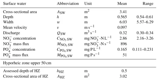
Table 2.Selected morphological and hydrological parameters of the testing site for the duration of the testing phase from 4–11 June 2015. Ranges are indicated for directly measured parameters, the remaining parameters have been calculated from listed means. HZ: hyporheic zone.
Surface water Abbreviation Unit Mean Range
Cross-sectional area ASW m2 3.41
Depth h m 0.565 0.54–0.61
Width w m 6.03 5.57–6.29
Mean velocity v m s−1 0.097
Discharge QSW m3s−1 0.32 0.30–0.34
NO−3 concentration CNO3SW mg NO −
3-N L
−1 2.86 2.16–3.26 NO−3 mass flux MNO3SW mg NO
−
3-N s
−1 896 PO−4 concentration CPO4SW mg P L
−1 0.165 0.111–0.231 PO−4 mass flux MPO4SW mg P s
−1 51
Hyporheic zone upper 50 cm
Assessed depth of HZ hHZ m 0.5
Cross-sectional area of HZ AHZ m2 3.02
was exhausted after 25.5 h (Supplement S1). We attributed the decrease of nutrients in the draining solution after break-through to biotic consumption of SRP (limiting nutrient) and NO−3. Under the laser scanning microscope growth of biofilm could be observed on obviously brown stained Purolite® beads of the columns from the biofouling experiment and to a very low degree on beads from the same column which ap-peared still clean (Supplement S1). Browning of Purolite® beads was not observed on Purolite®beads from the loading experiment (bigger columns, experiment not extended after break-through) but on the top 2 cm of the HPFM R2 after exposure at the study site.
3.2 Field testing
3.2.1 HPFMs and additional measurements HPFMs
Deployment required approximately 15 min per HPFM and could be conducted by two persons. The water depth during the installation was 40 to 100 cm, depending on the specific location in the stream.
The average horizontal water flow qx and nutrient flux
JN measured in the HPFM during the 7 day field testing
are illustrated in Fig. 3. All flux meter except 5 L showed decliningJNandqx with depth. Average horizontalqx was
76 cm d−1, ranging from 115 cm d−1in the shallowest layer
of 5 L to 20 cm d−1 in the deepest layer of AC4. Over the
7 days duration of the experiment, accumulated horizontal flow velocities of qx=8.4 cm 7 d−1 (±0.02 cm 7 d−1,
n=3) and nutrient fluxes of 29.4 mg NO−3-N m27 d−1 (±0.7 mg m2d−1, n=3) and 36.4 mg SRP m27 d−1 (±6.3 mg m2d−1, n=3) were detected in the control HPFM. Breaking these results down to dial values yields
qx=1.2 cm d−1(±0.003 cm d−1,n=3) and nutrient fluxes
of 4.2 mg NO−3-N m2d−1 (±0.1 mg m3d−1, n=3) and 5.2 mg SRP m2d−1 (±0.9 mg m2d−1, n=3). Comparing these fluxes to the JN values measured with the other
HPFM, an average 0.3 % of the uncorrected NO−3 flux and 5 % of the uncorrected SRP flux were attributed to tracer loss or nutrient accumulation resulting from transport, deployment, retrieval, analytical processing of samples and the background concentrations on the resin.
Vertical Darcy velocity (qy)
Vertical water flowqy in the streambed was predominantly
downward from January to October 2015. It was exclusively downward during the HPFM testing phase, ranging from 40 to 55 cm d−1. With this, vertical flowqy was slightly lower
than average horizontal flow qx. Resulting from the
rela-tionship between qy and qx the angle of hyporheic flow
(tanα=qy
qx)was 32
◦
downwards. Oxygen profiles
We observed strong diel variations in oxygen concentra-tion in the hyporheic zone. During several nights oxygen was nearly depleted (Fig. 4). The minima and maxima oxy-gen concentrations in the subsurface occurred contemporar-ily with the respective extremes in the surface water. Inter-estingly the amplitude in O2oscillation was higher at 45 cm
depths than at 25 cm depths. Multi-level samplers
Figure 3.Time-integrative measurements for 4–11 June 2015. Left: horizontal NO−3-N and SRP-P flux in mg m−2d−1through the resin HPFM R1(a), R2(b)and the layered HPFM L5(c)and L6(d). Right: corresponding Darcy velocitiesqxin cm d−1through the activated
carbon HPFM AC3(e)and AC4(f)and the layered HPFMs 5L(g)and 6L(h).
Figure 4. Time series of dissolved oxygen concentrations in the surface water (green) and the subsurface water (depth 25 cm, purple; depth 45 cm, orange) at the study site from 4–11 June 2015.
sampled pore water taken in June 2015 were higher than the average concentration derived from the HPFM. While the ex-pected increase of SRP and decrease of NO−3 and water flow with depths was observed in the HPFM, pore water extracted with the MLS showed no change over depth neither for NO−3 nor SRP. In the repeated manual pore-water samples taken in October (Fig. 6) NO−3 concentrations were uniformly lower in the early morning than in the afternoon, whereas SRP be-haved the other way round. This trend was consistent in both samplers even though the average concentration and distri-bution over depths differed between the samplers A and B.
On both sampling dates in June (4 and 11 June 2015) nei-ther SO24−nor boron showed a vertical gradient in concen-trations in the pore-water samples. SO24−concentrations of 170 mg L−1 on 4 June and 190 mg L−1on 11 June were in
Figure 5.Comparison between manually sampled pore water from MLS (red) and HPFM (blue) for NO−3-N (top) and SRP (bottom). Each MLS was sampled on 4 and 11 June 2015. Average surface water concentration during the deployment time and the concentra-tions at the time point of MLS sampling are marked in green.
Surface water chemistry
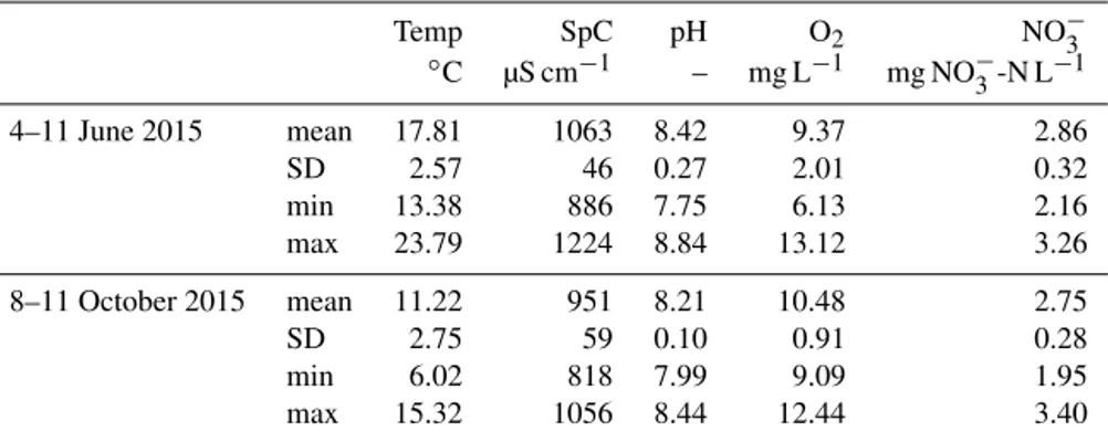
Temperature, O2and pH showed the expected diurnal
ampli-tudes whereas specific conductivity and NO−3 did not display a distinct diurnal pattern (Table 4).
3.2.2 Estimates of nitrate turnover rates based on HPFM measurements
With an average water flow of QHZ=2.65×10⁻⁵m3s−1
through the assessed upper 50 cm of the hyporheic zone and across the 6 m width of the stream, 0.008 % of water trans-ported in the river entered the hyporheic zone (Table 3).
While the average surface water concentration was 2.86 mg NO−3-N L−1, the average concentration in the sub-surface measured with the HPFM was only 1.39 mg NO−3 -N L−1. Assuming that the difference between surface and subsurface concentration arose from hyporheic consumption of infiltrating NO−3, the average removal rateRN was 52 %.
Figure 6.Concentrations of NO−3-N and SRP in time differentiat-ing manually taken pore-water samples from MLS A (bottom) and MLS B (top) on 8 October 2015. Corresponding surface water con-centrations are marked as vertical lines.
For SRP the average surface water concentration from 4 to 11 June 2015 was 0.165 mg P L−1, the average concentration
in the hyporheic zone was 0.11 mg P L−1.
4 Discussion
Table 3.Summarised parameters of NO−3 transport and removal through the upper 50 cm of the hyporheic zone at the test site for the testing phase from 4–11 June 2015. Ranges are indicated for directly measured parameters, the remaining parameters have been calculated from listed means.
Abbreviation Unit Mean Range
Water flow through HZ QHZ L s−1 0.0265
% of river water entering HZ %QHZ % 0.008
Horizontal Darcy velocity qx cm d−1 76 20–116
Average NO−3 concentration in the HZ CNO3HZ mg NO−3-N L−1 1.39 0.31–2.86 % NO−3 entering the HZ which is removed RN % 52
Potential NO−3 load entering HZ MHZ theory mg NO−3-N s−1 0.08 NO−3 load measured in HZ MHZ measured mg NO−3-N s−1 0.037
Table 4.Benchmark surface water parameters derived from the continuous sensor records from 4–11 June and 8–11 October 2015: Temp: temperature; SpC: specific conductivity; O2: dissolved oxygen.
Temp SpC pH O2 NO−3
◦C µS cm−1 – mg L−1 mg NO−
3-N L
−1
4–11 June 2015 mean 17.81 1063 8.42 9.37 2.86
SD 2.57 46 0.27 2.01 0.32
min 13.38 886 7.75 6.13 2.16
max 23.79 1224 8.84 13.12 3.26
8–11 October 2015 mean 11.22 951 8.21 10.48 2.75
SD 2.75 59 0.10 0.91 0.28
min 6.02 818 7.99 9.09 1.95
max 15.32 1056 8.44 12.44 3.40
they can be regarded as the method detection limit (MDL) (Greenberg et al., 1992). The MDL defines the lower limit for the use of HPFM in cases where nutrient fluxes are very low and deployment time cannot be extended. Based on the accumulated values detected in the control, the minimum de-ployment time can be estimated. In systems with high nutri-ent concnutri-entrations, usually the flow velocityqx will be the
limiting factor. In our application the MDL for qx derived
from the control was 8.4 cm for the complete deployment time (7 days). If the method inherited uncertainty should not be more than 5 % of the total measurement, the prod-uct of duration (in days) and velocity (in cm) should be at least 168 (20×8.4). As an example: if measured qx is
around 200 cm d−1, 1 day (24 h) of deployment is sufficient. The lowestqxdetected in our assessment was 21 cm d−1(in
HPFM AC4, see Fig. 3f), so that actually a deployment dura-tion of 8 days would have been optimal. The same estimadura-tion can additionally be derived for expected nutrient fluxes. In systems with low nutrient concentrations, it would be prefer-able to start estimating the minimum deployment time based on the nutrient fluxes. We recommend that a control HPFM is incorporated in each field application of HPFM in order to determine the specific MDL. The upper limit is given by the loading capacity of the resin or complete displacement of all resident alcohol tracers.
The high-nutrient background on the AC required the sep-aration of resin and AC in the HPFMs. We tested two dif-ferent HPFM designs in this study, of which each inherits designated characteristics being more or less beneficial for different specifications. The first approach consists of pairs of two HPFMs where one is used to assess the water flux and the second to capture nutrients, and is preferable if a highly resolved depth profile is needed (a heterogeneous hor-izontal flux in the vertical direction). Since this approach as-sumes that local horizontal heterogeneity is negligible in the range of 20–30 cm, we recommend this type only for the use in uniform systems such as channelised river reaches. Even in those systems however, small-scale variability in streambed and sediment characteristics can cause spatially heterogeneous flow distributions (Lewandowski et al., 2011; Mendoza-Lera and Mutz, 2013). The second approach with alternating nutrient sorbents and water flux measuring seg-ments is therefore preferable in most other cases as long as a high resolution over the vertical profile is not required. In general, several HPFMs should be grouped together in order to obtain representative results.
within the device and thereby increase spatial resolution, and second, because in a mixed texture of nutrient absorber and tracer carrier the antibacterial nature of the activated carbon would suppress biofouling on the absorbent. We observed substantial biofilm growth on the resin in the laboratory and on the top 2 cm of the field-deployed HPFM R2. The results of the column experiments suggest that biofilm growth on the resin porous media did not affect its loading capacity. Further, biofilm growth was only visible on columns which were run beyond breakthrough, suggesting that considerable biofouling only started after the loading capacity of the tracer was exhausted. R2 detected higher NO−3 fluxes in the top layer than the other HPFM. This could be due to contam-ination of the top layer of this HPFM with surface water (if the HPFM was not introduced sufficiently deep into the sediments). The further implication would be that this layer was exposed to much higher water and nutrient infiltration, so that the loading capacity was exhausted before the end of the experiment allowing biofilm accumulation. At the cur-rent state it is unclear to what extent the biofilm bound nu-trients can be extracted by the procedure used here. Further experiments would also be needed to clarify under which conditions biofilm growth can occur and if bacterial uptake, transformation and release of nutrients influence the con-centrations of nutrients inside the HPFM. HPFM segments on which biofilm is visible should be interpreted with cau-tion. Finally, identifying a procedure or materials which com-pletely inhibit biofouling will be an important step in the fur-ther development of HPFM.
In addition to instrumental adaptations we presented an installation procedure, which allows for smooth deployment with minimal disturbance of the system. Unlike typical well screen deployments where PFMs (Annable et al., 2005; Ver-reydt et al., 2013) or SBPFMs (Layton, 2015) have been in-serted into a screened plastic or steel casing, our technique enabled the direct contact of the HPFM with the surrounding river sediments. Disturbing the natural structure of the sed-iment, potentially resulting in artificial flow paths, is intrin-sic to all intrusive techniques, including HPFMs. Still, dis-pensing of a solid wall improves the integration of HPFMs in the natural system and prevents the generation of prefer-ential flow paths along the wall of the device. Additionally, the HPFMs include a measurement time that is long relative to the duration of the installation, suggesting that the pre-sented method causes lower disturbance compared to other intrusive measurements. While the installation of mini-drive points or heat pulse sensors in sediments coarser than sand may be difficult or even impossible and also proved unfea-sible at our field site, installation of the HPFM with the pre-sented technique was successful. The correction for conver-gence of flowlines into the device or diverconver-gence around it is relatively simple and already incorporated in the equation for the flux calculation. Heterogeneous permeability of the hyporheic zone around the HPFM does not distort the cor-rection term as long as the permeability of the surrounding is
coherently higher or coherently lower than the permeability of the HPFM matrix. Pre-measurements are therefore neces-sary for the selection of a suitable resin and tracer carrier. We believe that the presented approach and equations are ap-plicable for a wide range of field conditions. However, for very coarse sediments, a protection of the HPFM with a solid screen might still be preferred. If fine particles are observed to bypass the mesh and enter the HPFM, a finer mesh should be chosen. We did not observe clogging of the mesh or in-trusion of particles at our study, though in highly permeable systems with fine particle transport this might have to be con-sidered.
A major advantage of the HPFM method is highlighted by the findings of the 7 day long field testing. In June, we found discrepancies between the average concentrations measured in the HPFM and the concentration found using the MLS. From our measurements it is not possible to prove that the HPFM results are correct and the MLS results bi-ased. Nevertheless, the HPFM showed the expected decline inJN with depths, whereas the MLS pore-water
concentra-tions were similar at all depths. This can be related to two rea-sons. First, we might have sampled surface water which by-passed along the wall of the MLS. The question would then be why that happened in June but not in October; second, we might have sampled the MLS at a time point when the hyporheic zone was inactive in respect to nutrient process-ing. Considering the high diurnal amplitudes in hyporheic oxygen concentration, we assumed that the discrepancy be-tween HPFM and MLS arose from oscillations in hyporheic nutrient concentrations similar to the oxygen pattern. Mi-crobial consumption of O2 in the sediments can,
depend-ing on nutrient concentration in surface water and transfer of these nutrients to the sediments, result in O2 depletion
in the subsurface. Especially in nutrient-rich streams the re-lated diurnal oscillations in O2 concentration favour night
time denitrification in the hyporheic zone (Christensen et al., 1990; Laursen and Seitzinger, 2004; Harrison et al., 2005; O’Connor and Hondzo, 2008; Nimick et al., 2011). The re-dox conditions in the subsurface may also regulate the mobil-isation/demobilisation of phosphate (Smith et al., 2011). The repeated manual sampling of pore water from MLS in Octo-ber showed diurnal variations of SRP and NO−3 in the subsur-face of the testing reach, supporting the hypothesis that diur-nal cycles in benthic metabolism caused temporal variations in hyporheic SRP and NO−3 concentrations at our study site. As the majority of sampling is commonly conducted during daylight hours, night time conditions are under-represented in studies relying on single manual sampling events. Flux average concentrations can deviate by more than 50 % from estimates based on single event sampling, as was illustrated by comparison between our manual samples and the average pore-water concentrations calculated from the HPFM data.
few single time-specific snap shot samplings are conducted, the results may not realistically represent the overall condi-tions at the target site. Our comparison between MLS and HPFM reinforce the need for long-term recording of nutri-ent transport through the hyporheic zone. In general, most of our knowledge on hyporheic nutrient dynamics is based on measured surface water dynamics and models which project these dynamics on hyporheic processing. Theoretically, we could measure nutrient fluxes in the hyporheic zone and es-timate whole-stream uptake rates from these measurements. However, the substantially higher effort to obtain subsurface data is not justified in most cases. As long as the overall in-stream retention is the focus, surface water monitoring will remain the method of choice. Innovative tracer experiments may even allow quantifying hyporheic exchange in streams. Haggerty et al. (2009) proposed a “smart” tracer approach, where the injected substance resazurin converts irreversibly to resofurin under metabolic activity. While a promising tool for detecting metabolic activity at the sediment–water inter-face in streams, first, uncertainties about sorption and trans-formation characteristics of these tracers remain (Lemke et al., 2014) and second, those methods give no evidence about nutrient transport to those reactive sites.
Thus, whenever the nutrient processing function of the hy-porheic zone and its quantitative contribution to stream nu-trient retention is of interest, for example in the evaluation of restoration measures including a rehabilitation of the river bed, direct measurements of hyporheic fluxes are indispens-able. The HPFMs are a valuable approach that can be ef-ficiently used to characterise and quantify nutrient dynam-ics in a sediment system. We consider that a combination of HPFM, MLS and concurrent measurements of pore water oxygen concentrations, as presented in this study, provide a practical set-up to interpret hyporheic nutrient dynamics.
Like solute concentrations and water flow patterns, the ver-tical extension of the hyporheic zone varies in time and space and between different rivers and reaches. Our set-up assessed exclusively the upper 50 cm of the hyporheic zone. We found continuously decreasing NO−3 concentrations with depths, suggesting that this entire area (and potentially deeper) of the subsurface contained active sites for nitrate removal. While it was stated that denitrification is limited to the upper few cm of the hyporheic zone close to the sediment–water in-terface (Hill et al., 1998; Harvey et al., 2013), our results are in accordance to findings by Zarnetske et al. (2011b) and Kessler et al. (2012) who also report extended active hyporheic zones. Conducting collateral tracer tests, as sug-gested for example by Abbott et al. (2016), could deliver fur-ther evidence and characterise distinct flow paths. Neverthe-less, since vertical water movement was overall downward and the lowest concentrations of NO−3 were observed in the deepest segments of the HPFM, it is very likely that the hy-porheic zone at our study site extends deeper than the 50 cm evaluated. The length of an HPFM can easily be increased, depending on the individual site conditions.
Considering the high spatial heterogeneity of the hy-porheic zone, a larger number of HPFM would be needed to derive reliable and statistically supportable rates of hy-porheic nutrient dynamics. The following example aims to display further possibilities of interpreting HPFM measure-ments. At our study site, the hyporheic removal potentialRN
of more than 50 % of infiltrating NO−3 and 30 % of SRP suggests an active hyporheus. Evaluation of the effect of hyporheic removal activity on overall NO−3 removal in the stream or the normalisation of hyporheic uptake to a ben-thic area requires a flow path length. In the presented ex-ample, this length refers to the horizontal vector of the dis-tance the water travels in the subsurface before infiltrating the HPFM. The horizontal vector can be derived from the residence time of water and solutes in the hyporheic zone τHZand the horizontal Darcy velocityqx. Assuming a
down-ward flow direction, τHZ could be inferred from the
verti-cal Darcy velocityqyas assessed from the temperature
pro-filing and the hyporheic zone depths of 50 cm. Thereafter, τHZ conceptually corresponds to the time the water travels
through the hyporheic zone before exiting to groundwater andsHZ to the horizontal vector of the flow paths. The
ni-trate uptake rateUNO3-HZ(mg NO −
3-N m
−2d−1)is then the
difference between the theoretically transported NO−3 mass MNO3-HZ theor, which is the product of QHZ and CNO3-SW and the measured mass fluxMNO3-HZ real. During the testing phaseUNO3-HZ was calculated as 693 mg NO
−
3-N m
−2d−1.
The same procedure yields a removal (uptake or adsorption) rate for SRP ofUPO4-HZ=24 mg PO
−
4 m
−2d−1. Calculating UNO3-HZin the same way for each single depth assessed with the HPFM can deliver additional information about verti-cal gradients on nutrient processing rates and help to iden-tify the most active depth in hyporheic zone. UNO3-HZi of a particular layer in the hyporheic zone can be derived by the differences in uptake rate between the regarded layer and the overlying layer. For instance the removal rates attributed to the different layers of HPFM L6 would beUNO3-HZ15= 567 mg NO−3-N m−2d−1 in the shallow layer (0 to 15 cm depths),UNO3-HZ30=174 mg NO
−
3-N m
−2d−1 in the layer
from 15 to 30 cm depths and UNO3-HZ45=256 mg NO −
3
5 Conclusion and outlook
The role of the hyporheic zone as a hotspot for in-stream nu-trient cycling is indisputable (Mulholland et al., 1997; Fel-lows et al., 2001; Fischer et al., 2005; Rode et al., 2015). Quantitative and qualitative knowledge about the influence of mass transfer on hyporheic nutrient removal is crucial to manage streams and river, especially in the light of increasing worldwide morphological alterations (Borchardt and Pusch, 2009), eutrophication (Ingendahl et al., 2009) and sediment loading (Hartwig and Borchardt, 2015). Despite decades of research on hyporheic nutrient cycling, robust quantitative data on nutrient fluxes through the hyporheic zone are lim-ited, which is mainly due to methodological constraints in measuring nutrient concentrations and water flux in the sub-surface of streams (O’Connor et al., 2010; Boano et al., 2014; Gonzalez-Pinzon et al., 2015). Passive flux meters have the potential to fill the gap in measured quantitative nutrient fluxes to the reactive sites in the sediments of rivers. To date, HPFMs are virtually the only method which can simultane-ously capture nutrient and water flux through hyporheic zone within the same device and at the same spatial location. The field testing of several devices proved the general applica-bility of passive flux meters for quantifying NO−3 and PO−4 flux to reactive sites in the hyporheic zone. The hyporheic flux rates of nutrients and nitrate uptake rates measured in an agricultural 3rd-order stream were generally in agreement with rates reported in the literature. Our results clearly high-light the advantages of HPFM compared to commonly used methods (i.e. grab sampling of pore water and separate mea-surements of hyporheic exchange and Darcy velocities), first of all the capacity to integrate over longer time periods.
Quantifying nutrient flux to the potentially reactive sites in the hyporheic zone is an essential step to further improve our process-based knowledge on hyporheic nutrient cycling. In the future, long-term measurements of nutrient fluxes as obtained from HPFM can feed into and advance the transport part of nutrient cycling models.
We anticipate further improvement and increased use of passive flux meter approaches in order to advance conceptual models of nutrient cycling in the hyporheic zone. We demon-strated modifications which extended PFM application from groundwater to hyporheic zones. Current limitations related to the potential bias of results due to biofilm growth on sor-bents require further analysis for the identification of more suitable sorbents. While we focused on nutrients, PFMs may also be used for a wide range of other substances like con-taminants or trace elements.
Being labour efficient and attractive with respect to rela-tively low costs, numerous HPFMs can be efficiently used to cover larger areas and assess the degree of local hetero-geneity. Further, neither advanced technology, maintenance, or power supply are needed which can be extremely advan-tageous for the use in remote areas or study sites without infrastructure.
6 Data availability
All relevant data are either incorporated in figures/tables in the article or provided in the Supplement.
The Supplement related to this article is available online at doi:10.5194/bg-14-631-2017-supplement.
Competing interests. The authors declare that they have no conflict of interest.
Acknowledgements. We thank Uwe Kiwel for his technical support during the field work and Andrea Hoff and Christina Hoffmeister from the analytical department of the UFZ for their assistance in the laboratory experiments. We are also grateful for fruitful discussions with James Jawitz, Andreas Musolff, Christian Schmidt and Nico Trauth.
The article processing charges for this open-access publication were covered by a Research
Centre of the Helmholtz Association.
Edited by: T. J. Battin
Reviewed by: R. González-Pinzón, J. Rozemeijer, J. Lewandowski, and one anonymous referee
References
Abbott, B. W., Baranov, V., Mendoza-Lera, C., Nikolakopoulou, M., Harjung, A., Kolbe, T., Balasubramanian, M. N., Vaessen, T. N., Ciocca, F., Campeau, A., Wallin, M. B., Romeijn, P., Antonelli, M., Gonçalves, J., Datry, T., Laverman, A. M., De Dreuzy, J.-R., Hannah, D. M., Krause, S., Oldham, C., and Pinay, G.: Using multi-tracer inference to move beyond single-catchment ecohydrology, Earth-Sci. Rev., 160, 19–42, 2016. Alexander, R. B., Böhlke, J. K., Boyer, E. W., David, M. B.,
Har-vey, J. W., Mulholland, P. J., Seitzinger, S. P., Tobias, C. R., Tonitto, C., and Wollheim, W. M.: Dynamic modeling of nitro-gen losses in river networks unravels the coupled effects of hy-drological and biogeochemical processes, Biogeochemistry, 93, 91–116, doi:10.1007/s10533-008-9274-8, 2009.
Angermann, L., Krause, S., and Lewandowski, J.: Application of heat pulse injections for investigating shallow hyporheic flow in a lowland river, Water Resour. Res., 48, W00P02, doi:10.1029/2012WR012564, 2012.
Annable, M. D., Hatfield, K., Cho, J., Klammler, H., Parker, B. L., Cherry, J. A., and Rao, P. S. C.: Field-Scale Evaluation of the Pas-sive Flux Meter for Simultaneous Measurement of Groundwater and Contaminant Fluxes, Environ. Sci. Technol., 39, 7194–7201, doi:10.1021/es050074g, 2005.
Pollehne, F.: Nutrient budgets for European seas: A measure of the effectiveness of nutrient reduction policies, Mar. Pollut. Bull., 56, 1609–1617, doi:10.1016/j.marpolbul.2008.05.027, 2008. Basu, N. B., Rao, P. S. C., Thompson, S. E., Loukinova, N. V.,
Don-ner, S. D., Ye, S., and Sivapalan, M.: Spatiotemporal averaging of in-stream solute removal dynamics, Water Resour. Res., 47, W00J06, doi:10.1029/2010WR010196, 2011.
Bernot, M. J. and Dodds, W. K.: Nitrogen retention, removal and saturation in lotic ecosystems, Ecosystems, 8, 442–453, doi:10.1007/s10021-003-0143-y, 2005.
Binley, A., Ullah, S., Heathwaite, A.L., Heppell, C., Byrne, P., Landsdown, K., Timmer, M., and Zhang, H.: Revealing the spa-tial variability of water fluxes at the groundwater-surface water interface, Water Resour. Res., 49, 3978–3992, 2013.
Boano, F., Harvey, J. W., Marion, A., Packman, A. I., Revelli, R., Ridolfi, L., and Worman, A.: Hyporheic flow and transport pro-cesses: Mechanisms, models and biogeochemical implications, Rev. Geophys., 52, 603–679, doi:10.1002/2012rg000417, 2014. Böhlke, J. K., Antweiler, R. C., Harvey, J. W., Laursen, A. E., Smith,
L. K., Smith, R. L., and Voytek, M. A.: Multi-scale measure-ments and modeling of denitrification in streams with varying flow and nitrate concentration in the upper Mississippi River basin, USA, Biochemistry, 93, 117–141, doi:10.1007/s10533-008-9282-8, 2009.
Borchardt, D. and Pusch, M. T.: An integrative, interdisciplinary research approach for the identification of patterns, processes and bottleneck functions of the hyporheic zone of running waters, Adv. Limnol., 61, 2009.
Boyer, E. W., Alexander, R. B., Parton, W. J., Li, C., Butterbach-Bahl, K., Donner, S. D., Skaggs, R. W., and Grosso, S. J. D.: Modeling denitrification in terrestrial and aquatic ecosystems at regional scales, Ecol. Appl., 16, 2123–2142, 2006.
Brookshire, E. N. J., Valett, H. M., and Gerber, S.: Maintenance of terrestrial nutrient loss signatures during in-stream transport, Ecology, 90, 293–299, doi:10.1890/08-0949.1, 2009.
Cho, J., Annable, M. D., Jawitz, J. W., and Hatfield, K.: Passive flux meter measurement of water and nutrient flux in saturated porous media: Bench-scale laboratory tests, J. Environ. Qual., 36, 1266– 1272, doi:10.2134/jeq2006.0370, 2007.
Christensen, P. B., Nielsen, L. P., Sorensen, J., and Revsbech, N. P.: Denitrification in nitrate-rich streams – dirunal and seasonal vari-ation related to benthic oxygen metabolism, Limnol. Oceanogr., 35, 640–651, 1990.
Clark, C. J., Hatfield, K., Annable, M. D., Gupta, P., and Chirenje, T.: Estimation of arsenic contamination in groundwater by the Passive flux meter, Environmental Forensics, 6, 77–82, doi:10.1080/15275920590913930, 2005.
Cook, P. L. M., Wenzhoefer, F., Rysgaard, S., Galaktionov, O. S., Meysman, F. J. R., Eyre, B. D., Cornwell, J., Huettel, M., and Glud, R. N.: Quantification of denitrification in permeable sedi-ments: Insights from a two-dimensional simulation analysis and experimental data, Limnol. Oceanogr.-Meth., 4, 294–307, 2006. Cooke, J. G. and White, R. E.: Spatial distribution of denitrifying activity in a stream draining an agricultural catchment, Freshwa-ter Biol., 18, 509–519, 1987.
Covino, T., McGlynn, B., and Baker, M.: Separating phys-ical and biologphys-ical nutrient retention and quantifying up-take kinetics from ambient to saturation in successive
moun-tain stream reaches, J. Geophys. Res.-Biogeo., 115, G04010, doi:10.1029/2009jg001263, 2010.
Duff, J. H. and Triska, F. J.: Denitrification in sediments from the hyporheic zone adjacent to a small forested stream, Can. J. Fish. Aquat. Sci., 47, 1140–1147, 1990.
Duff, J. H., Murphy, F., Fuller, C. C., and Triska, F. J.: A mini drive-point sampler for measuring pore water solute concentrations in the hyporheic zone of sand-bottom streams, Limnol. Oceanogr., 43, 1378–1383, 1998
Ensign, S. H. and Doyle, M. W.: Nutrient spiraling in streams and river networks, J. Geophys. Res.-Biogeo., 111, G04009, doi:10.1029/2005jg000114, 2006.
Fellows, C. S., Valett, H. M., and Dahm, C. N.: Whole-stream metabolism in two mountain streams: Contribution of the hy-porheic zone, Limnol. Oceanogr., 46, 523–531, 2001.
Fetter, C. W.: Applied Hydrogeology, 4th Edn., New Jersey: Pren-tice Hall, 2001.
Fleckenstein, J. H., Krause, S., Hannah, D. M., and Boano, F.: Groundwater-surface water interactions: New methods and mod-els to improve understanding of processes and dynamics, Adv. Water Resour., 33, 1291–1295, 2010.
Findlay, S. E. G., Mulholland, P. J., Hamilton, S. K., Tank, J. L., Bernot, M. J., Burgin, A. J., Crenshaw, C. L., Dodds, W. K., Grimm, N. B., McDowell, W. H., Potter, J. D., and Sobota, D. J.: Cross-stream comparison of substrate-specific denitrification potential, Biogeochemistry, 104, 381–392, doi:10.1007/s10533-010-9512-8, 2011.
Fischer, H., Kloep, F., Wilzcek, S., and Pusch, M. T.: A river’s liver – microbial processes within the hyporheic zone of a large low-land river, Biogeochemistry, 76, 349–371, doi:10.1007/s10533-005-6896-y, 2005.
Fischer, J., Borchardt, D., Ingendahl, D., Ibisch, R., Saenger, N., Wawra, B., and Lenk, M.: Vertical gradients of nutrients in the hyporheic zone of the River Lahn (Germany): Relevance of surface versus hyporheic conversion processes, Adv. Limnol., 01/2009, 105–118, 2009.
Galloway, J. N., Aber, J. D., Erisman, J. W., Seitzinger, S. P., Howarth, R. W., Cowling, E. B., and Cosby, B. J.: The nitrogen cascade, Bioscience, 53, 341–356, 2003.
Garcia-Ruiz, R., Pattinson, S. N., and Whitton, B. A.: Kinetic pa-rameters of denitrification in a river continuum, Appl. Environ. Microbiol., 64, 2533–2538, 1998a.
Gonzalez-Pinzon, R., Ward, A. S., Hatch, C. E., Wlostowski, A. N., Singha, K., Gooseff, M. N., Haggerty, R., Harvey, J. W., Cirpka, O. A., and Brock, J. T.: A field comparison of multiple techniques to quantify groundwater-surface-water interactions, Freshwater Sci., 34, 139–160, doi:10.1086/679738, 2015.
Grant, S. B., Stolzenbach, K., Azizian, M., Stewardson, M. J., Boano, F., and Bardini, L.: First-order contaminant removal in the hyporheic zone of streams: Physical insights from a sim-ple analytical model, Environ. Sci. Technol., 48, 11369–11378, doi:10.1021/es501694k, 2014.
Greenberg, A. E., Clesceri, L. S., and Eaton, A. D.: Standard Meth-ods for the Examination of Water and Wastewater, American Public Health Association, 18th Edn., Washington, D.C., 1992. Haggerty, R., Marti, E., Argerich, A., Von Schiller, D., and Grimm,