www.biogeosciences.net/14/45/2017/ doi:10.5194/bg-14-45-2017
© Author(s) 2017. CC Attribution 3.0 License.
Development and evaluation of an ozone deposition scheme
for coupling to a terrestrial biosphere model
Martina Franz1,2, David Simpson4,5, Almut Arneth6, and Sönke Zaehle1,3
1Biogeochemical Integration Department, Max Planck Institute for Biogeochemistry, Jena, Germany 2International Max Planck Research School (IMPRS) for Global Biogeochemical Cycles, Jena, Germany 3Michael Stifel Center Jena for Data-driven and Simulation Science, Jena, Germany
4EMEP MSC-W, Norwegian Meteorological Institute, Oslo, Norway
5Department of Earth & Space Sciences, Chalmers University of Technology, Gothenburg, Sweden
6Karlsruhe Institute of Technology (KIT), Department of Atmospheric Environmental Research (IMK-IFU),
Garmisch-Partenkirchen, Germany
Correspondence to:Martina Franz ([email protected])
Received: 18 July 2016 – Published in Biogeosciences Discuss.: 28 July 2016
Revised: 11 November 2016 – Accepted: 12 December 2016 – Published: 6 January 2017
Abstract.Ozone (O3) is a toxic air pollutant that can
dam-age plant leaves and substantially affect the plant’s gross pri-mary production (GPP) and health. Realistic estimates of the effects of tropospheric anthropogenic O3 on GPP are thus
potentially important to assess the strength of the terrestrial biosphere as a carbon sink. To better understand the impact of ozone damage on the terrestrial carbon cycle, we devel-oped a module to estimate O3uptake and damage of plants
for a state-of-the-art global terrestrial biosphere model called OCN. Our approach accounts for ozone damage by calculat-ing (a) O3transport from 45 m height to leaf level, (b) O3
flux into the leaf, and (c) ozone damage of photosynthesis as a function of the accumulated O3uptake over the lifetime of
a leaf.
A comparison of modelled canopy conductance, GPP, and latent heat to FLUXNET data across European forest and grassland sites shows a general good performance of OCN including ozone damage. This comparison provides a good baseline on top of which ozone damage can be evaluated. In comparison to literature values, we demonstrate that the new model version produces realistic O3surface resistances,
O3deposition velocities, and stomatal to total O3flux ratios.
A sensitivity study reveals that key metrics of the air-to-leaf O3 transport and O3 deposition, in particular the stomatal
O3 uptake, are reasonably robust against uncertainty in the
underlying parameterisation of the deposition scheme. Nev-ertheless, correctly estimating canopy conductance plays a
pivotal role in the estimate of cumulative O3uptake. We
fur-ther find that accounting for stomatal and non-stomatal up-take processes substantially affects simulated plant O3
up-take and accumulation, because aerodynamic resistance and non-stomatal O3destruction reduce the predicted leaf-level
O3concentrations. Ozone impacts on GPP and transpiration
in a Europe-wide simulation indicate that tropospheric O3
impacts the regional carbon and water cycling less than ex-pected from previous studies. This study presents a first step towards the integration of atmospheric chemistry and ecosys-tem dynamics modelling, which would allow for assessing the wider feedbacks between vegetation ozone uptake and tropospheric ozone burden.
1 Introduction
Tropospheric ozone (O3) is a highly reactive and toxic gas.
In western Europe, tropospheric O3 levels increased
ap-proximately by a factor 2 to 5 from pre-industrial values to the 1990s (Cooper et al., 2014; Marenco et al., 1994; Stae-helin et al., 1994) (although the low values at the start of this period are very uncertain) and approximately doubled between 1950 and 1990s in the Northern Hemisphere (Par-rish et al., 2012; Cooper et al., 2014). The major causes for this increased O3 formation are the increased emission
of O3 precursor trace gases such as NOx and CO,
primar-ily from combustion sources, non-methane volatile organic compounds from anthropogenic sources (combustion, sol-vents), and methane emissions from agriculture and industry (Fusco and Logan, 2003; Vingarzan, 2004). For instance, in western Europe, NOx emissions rose by a factor of 4.5
be-tween 1955 and 1985 (Staehelin et al., 1994). In addition, downward transport of O3from the stratosphere to the
tropo-sphere (Vingarzan, 2004; Young et al., 2013) and interconti-nental transport (Vingarzan, 2004; Jenkin, 2008; Fiore et al., 2009) can increase local and regional O3concentrations.
A commonly observed consequence of elevated levels of O3exposure is a decline in net photosynthesis (Morgan et al.,
2003; Wittig et al., 2007), which may result from the damage of the photosynthetic apparatus or increased respiration due to the production of defence compounds and investments in injury repair (Wieser and Matyssek, 2007; Ainsworth et al., 2012). The reduction in net photosynthesis results in reduced growth and hence a reduced leaf area and plant biomass (Morgan et al., 2003; Lombardozzi et al., 2013; Wittig et al., 2009). The tight coupling between photosynthesis and stom-atal conductance further affects canopy conductance, and thereby transpiration rates (Morgan et al., 2003; Wittig et al., 2009; Lombardozzi et al., 2013), likely affecting the ecosys-tem water balance.
Due to its phytotoxic effect, elevated O3levels as a
con-sequence of anthropogenic air pollution may affect the land carbon cycle and potentially reduce the net land carbon up-take capacity (Sitch et al., 2007; Arneth et al., 2010; Simp-son et al., 2014a), which currently corresponds to about a quarter of the anthropogenic fossil fuel emissions as a result of a sustained imbalance between photosynthetic carbon up-take and carbon loss through respiration and disturbance pro-cesses (Le Quéré et al., 2015). However, the extent to which O3 affects plant health regionally and thereby alters
terres-trial biogeochemistry and the terresterres-trial water balance is still subject of large uncertainty (Simpson et al., 2014a).
A number of O3 exposure indices have been proposed
to assess the potential detrimental effect of tropospheric O3 on the plants (LRTAP Convention, 2010; Mills et al.,
2011b). In Europe, the standard method of these indices is the concentration-based AOTX (ppb h) (accumulated O3
con-centration over a threshold ofXppb), which relates the
free-air O3concentration to observed plant damage. Models
as-sessing ozone damage to gross or net primary production based on AOTX have been used for many years and indi-cate that substantial reduction in plant growth and carbon
sequestration occurs globally and may reach reductions of more than 40 % at O3 hotspots (Felzer et al., 2004, 2005;
Ren et al., 2011; Anav et al., 2011).
A significant caveat of concentration-based assessments of ozone toxicity effects is that species differ vastly in their canopy conductance as well as regional provenances of species. Stomatal control of the leaf gas exchange regu-lates photosynthesis and varies, inter alia, with plant-specific photosynthetic capacity and intrinsic water-use efficiency of photosynthesis; phenology; and environmental factors such as incident light, atmospheric vapour pressure deficit (VPD), and air temperature. The consequent differences in stomatal conductance implies that the actual O3 dose, and thus the
level of ozone-related damage, differs between species ex-posed to similar atmospheric O3concentrations (Wieser and
Havranek, 1995). The O3 dose, which is the integral of the
instantaneous O3stomatal flux over a given period of time,
has been observed to strongly correlate with the amount of injury of a plant suggesting that plants with higher stomatal conductance are subject to higher doses and hence more sus-ceptible to injury (Reich, 1987; Wittig et al., 2009).
Accounting for the O3 dose rather than the O3exposure
in assessments of ozone damage results in diverging regional patterns of ozone damage, as regions with the highest expo-sure (O3concentrations) do not always coincide with regions
of high uptake (Emberson et al., 2000; Mills et al., 2011a; Simpson et al., 2007). Regions with low AOT40 (AOTX above a threshold of 40 ppb) values might show moderate to high values of O3uptake because the flux approach
ac-counts for climatic conditions that enable high stomatal con-ductances and hence high values of O3uptake (Mills et al.,
2011a). Observed ozone damage in the field seems to be bet-ter correlated with flux-based risk assessment compared to concentration-based methods (Mills et al., 2011a). Following this the LRTAP Convention recommends flux-based methods as the preferred tool for risk assessment (LRTAP Convention, 2010).
When calculating the O3uptake into the plants, it is
impor-tant to consider that stomatal uptake is not the only surface sink of O3. O3destruction also occurs at non-stomatal
sur-faces such as the leaves’ cuticle and soil surface. The stom-atal flux represents approximately half of the total O3flux to
the surface (Gerosa et al., 2004; Fowler et al., 2009; Cies-lik, 2004; Simpson et al., 2003). Accounting for this non-stomatal O3deposition reduces the amount of O3uptake into
the plants by reducing the surface O3concentration
(Tuovi-nen et al., 2009) and thus has the potential to affect flux-based ozone damage estimates.
A further challenge in estimating plant damage related to O3uptake is that plants differ in their ability to remove any
ROS from the leaf before damage of leaf cellular organs is incurred (Luwe and Heber, 1995). Conceptually, one can de-scribe the capacity as a plant-specific O3 dose with which
produc-tion of defence compounds increases respiraproduc-tion costs and following this reduces net primary production what may re-sult in reduced growth and biomass (Ainsworth et al., 2012). Ozone damage is only incurred once the O3flux into the leaf
exceeds this dose. A commonly used index to assess flux-based damage to plants is the PODy (phytotoxic ozone dose, nmol m−2s−1), which gives the accumulated O3 flux above
a threshold of Ynmol m−2s−1 for all daylight hours and a
given time period. Common threshold values for PODy range from 1 to 6 nmol m−2s−1(Pleijel et al., 2007; LRTAP
Con-vention, 2010; Mills et al., 2011b), depending on the specific species sensitivity to O3.
Only a few terrestrial biosphere models have adopted the flux approach to relate O3 exposure to plant damage and
thus estimate O3-induced reductions in terrestrial carbon
se-questration in a process-based manner. Sitch et al. (2007) developed a version of the JULES model in which stom-atal O3uptake directly affects net primary production (NPP),
thereby ignoring the effect of reduced photosynthesis under elevated levels of O3 on water fluxes. Lombardozzi et al.
(2015) proposed a revised version of the Community Land Model (CLM), in which O3imposes fixed reductions to net
photosynthesis for two out of three modelled plant types. At-mospheric O3concentrations and the amount of cumulated
O3 uptake directly affect net photosynthesis only for one
plant type.
In this paper, we present a new, globally applicable model to calculate O3 uptake and damage in a process-oriented
manner, coupled to the terrestrial energy, water, carbon, and nitrogen budget of the OCN terrestrial biosphere model (Za-ehle and Friend, 2010).
In this model, the canopy O3abundance is calculated using
aerodynamic resistance and surface resistances to soil sur-face, vegetation surfaces, and stomatal cavities to take ac-count of non-stomatal O3destruction. Canopy O3abundance
is used to simulate stomatal O3uptake given instantaneous
values of net photosynthesis and stomatal conductance. O3
uptake and its effect on net photosynthesis is then calculated based on an extensive meta-analysis across 28 tree species by Wittig et al. (2007) considering the ability of plants to detoxify a proportion of the O3dose (Sitch et al., 2007).
We first give a detailed overview of the ozone scheme (Sect. 2.1); evaluate modelled gross primary production (GPP), canopy conductance, latent heat fluxes, and leaf area index (LAI) against data from the FLUXNET database (Bal-docchi et al., 2001) to test the ability of the model to simulate observed values of key components affecting calculate O3
uptake (Sect. 3.1); evaluate the simulated O3metrics against
reported values in the literature (Sect. 3.2); provide a sen-sitivity analysis of critical variables and parameters of the deposition model to evaluate the reliability of simulated val-ues of O3uptake (Sect. 3.3); give an estimate of the effect of
the present-day O3burden on European GPP and
transpira-tion(Sect. 3.4); and estimate the impact of using the O3
depo-sition scheme on O3uptake and cumulated uptake (Sect. 3.5).
2 Methods
We developed an ozone deposition and leaf-uptake module for the terrestrial biosphere model OCN (Zaehle and Friend, 2010). OCN is a further development of the land-surface scheme ORCHIDEE (O) (Krinner et al., 2005), and simulates the terrestrial coupled carbon (C), nitrogen (N), and water cycles for 12 plant functional types (PFTs) driven by climate data, atmospheric composition (N deposition, as well as at-mospheric CO2 and O3 burden), and land-use information
(land cover and fertiliser application).
In OCN net photosynthesis is calculated for shaded and sunlit leaves in a multi-layer canopy with up to 20 layers (each with a thickness of up to 0.5 leaf area index) follow-ing a modified Farquhar scheme and considerfollow-ing the light profiles of diffuse and direct radiation (Zaehle and Friend, 2010). Photosynthetic capacity depends on leaf nitrogen con-centration and leaf area, which are both affected by ecosys-tem available N. Increases in leaf nitrogen content enable higher net photosynthesis and higher stomatal conductance per unit leaf area. This in turn affects transpiration as well as O3uptake and ozone damage estimates. Leaf N is highest in
the top canopy and monotonically decreases with increasing canopy depth. Following this, stomatal conductance and O3
uptake is generally highest in the upper canopy and lowest in the bottom of the canopy.
The O3 and N-deposition data used for this study are
provided by the EMEP MSC-W (European Monitoring and Evaluation Programme Meteorological Synthesizing Centre – West) chemical transport model (CTM) (Simpson et al., 2012). The O3 flux and deposition modules used in the
EMEP model are advanced compared to most CTMs, and have been documented in a number of papers (Emberson et al., 2001; Tuovinen et al., 2004, 2009; Simpson et al., 2007, 2012; Klingberg et al., 2008). The ozone deposition scheme for OCN is adapted from the model used by EMEP MSC-W (Simpson et al., 2012) to fit the land-surface charac-teristics and process descriptions of the ORCHIDEE model. The leaf-level ozone concentrations computed by EMEP can not directly be used by OCN, since EMEP and OCN differ in a number of properties, as for instance in the number of sim-ulated PFTs, and importantly their ecophysiological process representation. Both models differ in the simulation of vari-ous ecosystem processes (e.g. phenology, canopy processes, biogeochemical cycles, and vegetation dynamics, which are more explicitly represented in OCN), which in sum impact stomatal and non-stomatal ozone deposition and through this the leaf-level ozone concentration. A possible further devel-opment of the new OCN is the coupling to a CTM to allow for a consistent simulation of tropospheric O3 burden and
2.1 Ozone module
The ozone deposition scheme calculates O3deposition to the
leaf surface from the free atmosphere, represented by the O3
concentration at the lowest level of the atmospheric CTM, taken to be at 45 m above the surface. The total O3dry
depo-sition flux (Fg) to the ground surface is calculated as
Fg =VgχatmO3, (1)
whereχatmO3 is the O3concentration at 45 m andVgis the
de-position velocity at that height. In OCN Vg is taken to be
dependent on the aerodynamic resistance (Ra), canopy-scale
quasi-laminar layer resistance (Rb) and the compound
sur-face resistance (Rc) to O3deposition.
Vg= 1
Ra+Rb+Rc (2)
Rbis calculated from the friction velocity (u∗) as
Rb = 6
u∗
. (3)
TheRabetween 45 m height and the canopy is not computed
by OCN and is inferred from the logarithmic wind profile (for more details see Appendix A). Rc is calculated as the
sum of the parallel resistances to stomatal/canopy (1/GOc3)
and non-stomatal O3uptake (1/Gns) (Simpson et al., 2012,
Eq. 55):
Rc= 1
GOc3+Gns
. (4)
The stomatal conductance to O3GOst3 (m s−1) is computed by
OCN (Zaehle and Friend, 2010) as
GOst3 =g1f (2)f (qair)f (Ci)f (height)An,sat
1.51 , (5)
whereGOst3is calculated as a function of net photosynthesis at
saturatingCi(An,sat), whereg1is the intrinsic slope between
AnandGst. It further depends on a number of scalars to
ac-count for the effect of soil moisture (f (2)), water transport
limitation with canopy height (f (height)), and atmospheric
drought (f(qair)), as well as an empirical non-linear
sensitiv-ity to the internal leaf CO2concentration (f (Ci)), all as
de-scribed in Friend and Kiang (2005). The factor 1.51 accounts for the different diffusivity of O3from water vapour
(Mass-man, 1998). The canopy conductance to O3 GOc3 is
calcu-lated by summing theGOst3of all canopy layers. To yield
rea-sonable conductance values in OCN compared to FLUXNET data (see Sect. 3.1), the original intrinsic slope between An
andGccalledαin Friend and Kiang (2005) is adapted such
thatg1= 0.7α.
The non-stomatal conductanceGnsfollows the EMEP
ap-proach (Simpson et al., 2012, Eq. 60) and represents the O3
fluxes between canopy-air space and surfaces other than the stomatal cavities. The model accounts for O3destruction on
the leaf surface (rext), within-canopy resistance to O3
trans-port (Rinc), and ground surface resistance (Rgs):
Gns = SAI
rext +
1
Rinc+Rgs, (6)
where the surface area index (SAI) is equal to the LAI for herbaceous PFTs (grasses and crops) and SAI=LAI+1 for
tree PFTs according to Simpson et al. (2012) in order to account for O3 destruction on branches and stems. Unlike
EMEP, we do not apply a day of the growing season con-straint for crop exposure to O3, which in OCN is accounted
for by the simulated phenology and seasonality of photosyn-thesis. The external leaf resistance (rext) per unit surface area
is calculated as
rext =rext,bFT, (7)
where the base external leaf resistance (rext,b) of 2500 m s−1
is scaled by a low-temperature correction factorFT and
FT =e−0.2(1+Ts), (8)
with 1≤FT ≤2 andTs the 2 m air temperature (◦C
Simp-son et al., 2012, Eq. 60). For temperatures below−1◦C
non-stomatal resistances are increased up to two times (Simpson et al., 2012; Zhang et al., 2003). The within-canopy resis-tance (Rinc) is calculated as
Rinc =bSAIh u∗
, (9)
wherebis an empirical constant (set to 14 s−1) andhis the
canopy height in m. The ground-surface resistanceRgsis
cal-culated as
Rgs = 1−2fsnow
FTRˆgs
+2fsnow
Rsnow (10)
(Simpson et al., 2012, Eq. 59).Rˆgsrepresents base values of Rgs and takes values of 2000 s m−1for bare soil, 200 s m−1
for forests and crops, and 1000 s m−1 for non-crop grasses
(Simpson et al., 2012, Suppl.). As in EMEP, the ground-surface resistance of O3to snow (Rsnow) is set to a value of
2000 s m−1according to Zhang et al. (2003).f
snowis
calcu-lated from the actual snow depth (sd) simulated by OCN, and
the maximum possible snow depth (sd, max):
fsnow= sd
sd,max (11)
with the constraint of 0≤fsnow≤0.5 to prevent negative
values in the first fraction of Eq. (10).sd,max is taken to be
Given these resistances, the canopy O3 concentration
(χcO3, nmol m−3) is then calculated based on a constant flux
assumption:
χO3
c =χatmO3(1−
Ra
Ra+Rb+Rc). (12)
χcO3 and the stomatal conductance to O3 (GOst3 in m s−1)
are used to calculate the O3flux into the leaf cavities (Fst,
nmol m−2s−1):
Fst=(χO3
c −χiO3)G O3
st . (13)
According to Laisk et al. (1989) the leaf internal O3
concen-tration (χiO3) is assumed to be zero.
The OCN implementation of deposition and flux described above is a simplification of the deposition system used by EMEP in order to fit the process representation of OR-CHIDEE, from which OCN has inherited its biophysical modules. The external leaf resistance is not included in the calculation of Fst (Tuovinen et al., 2007, 2009), which
re-sults in an overestimation of stomatal O3 uptake. Further,
OCN’s calculation ofRais based upon neutral stability
con-ditions (see Appendix), whereas the EMEP model makes use of rather detailed stability correction factors. However, a se-ries of calculations with the full EMEP model have shown that the uncertainties associated with these simplifications are small, typically 0.5–5 mmol m−2. As base-case values of
POD0 are typically ca. 30–50 mmol m−2in EU regions, these
approximations do not seem to be a major cause of error, at least in regions with substantial ozone (and carbon) uptake. The full coupling of OCN to a CTM would be desirable to eliminate this bias and allow for a consistent calculation of tropospheric and surface near O3burdens.
2.2 Relating stomatal uptake to leaf damage
An accumulation ofFstover time gives the accumulated
up-take of O3for a particular canopy layer (CUOl, mmol m−2),
or forl=1 (top canopy layer) the phytotoxic O3dose (POD,
mmol m−2):
dCUOl
dt =(1−fnew)CUOl+cFst,l, (14)
wherec=10−6converts from nmol to mmol and the
integra-tion time step is 1800 s.
The phenology of leaves is accounted for by assuming that emerging leaves are undamaged and by reducing the CUOl by the fraction of newly developed leaves per time
step and layer (fnew). Furthermore, deciduous PFTs shed all
CUO at the end of the growing season and grow undamaged leaves the next spring. Evergreen PFTs shed proportionate amounts of CUO during the entire year whenever new leaves are grown.
The full canopy cumulative uptake of O3is calculated by
summing CUOlover all present canopy layers (n):
CUO= n
X
l=1
CUOl. (15)
The CUOlis used to approximate the damage to net
pho-tosynthesis (An) by using the damage relationship of Wittig
et al. (2007):
dlO3 = 0.22CUOl+6.16
100 , (16)
where the factor 100 scales the percentage values of damage to fractions. Net photosynthesis accounting for ozone dam-age (AOn3) is then calculated by subtracting the damage
frac-tion from the undamaged value ofAn:
AOn,3l =An,l(1−dlO3). (17)
SinceGstandAnare tightly coupled (see Eq. 5), a damage
ofAnresults in a simultaneous reduction inGst. The
canopy-scale O3 flux into the leaf cavities (FstC) is calculated by
summingFstof all canopy layers, similar to the aggregation
ofAn,landGstand CUOl. Canopy O3concentration, O3
up-take, canopy cumulative O3uptake (CUO), and damage to
net photosynthesis are solved iteratively to account for the feedbacks between ozone damage, canopy conductance and canopy-air O3concentrations.
Note that CUO and POD can be directly compared to es-timates according to the LRTAP Convention (2010) nota-tion when analysing only the top canopy layer (Mills et al., 2011b).
2.3 Sensitivity analysis
A sensitivity analysis is conducted to estimate the sensitiv-ity of the modelled plant O3 uptake to the parameterisation
of the model, to establish the robustness of the model, and to identify the most influential parameters. Three parame-ters (ground-surface resistance (Rˆgs), external leaf resistance
(rext), and empirical constant (b); see Eqs. 10, 6, and 9
re-spectively) and three modelled quantities (canopy conduc-tance (Gc), aerodynamic resistance (Ra), and canopy-scale
quasi-laminar layer resistance (Rb); see Eqs. 5, 2), with
con-siderable uncertainty due to the underlying parameters used to calculate these quantities, are perturbed within±20 % of
their central estimate.
A set of 100 parameter combinations is created with a Latin hypercube sampling method (McKay et al., 1979), si-multaneously perturbing all six parameter values (R package: FME; function: Latinhyper). For each parameter combina-tion, a transient run (see Sect. 2.4) is performed creating an ensemble of estimates for the key prognostic variablesFstC
(Eq. 13),Rc(Eq. 4),Vg(Eq. 2) and the O3flux ratio (FR)
cal-culated as the ratio ofFstCand the total O3flux to the surface
The summer months June, July, and August (JJA) are se-lected from the simulation output and used for further analy-sis. For each prognostic variable (FstC,Rc,Vg,FR), the
sen-sitivity to changes in all six perturbed parameters/variables is estimated by calculating partial correlation coefficients (PCCs) and partial ranked correlation coefficients (PRCCs) (Helton and Davis, 2002). PCCs record the linear relation-ship between two variables where the linear effects of all other variables in the analysis are removed (Helton and Davis, 2002). In the case of nonlinear relationships, PRCCs can be used, which implies a rank transformation to linearise any monotonic relationship, such that the regression and cor-relation procedures as in the PCCs can follow (Helton and Davis, 2002). We estimate the magnitude of the parameter effect by creating mean summer values of the four prognostic variables for each sensitivity run, and regressing these values against the corresponding parameter/variable scaling values of the respective model run.
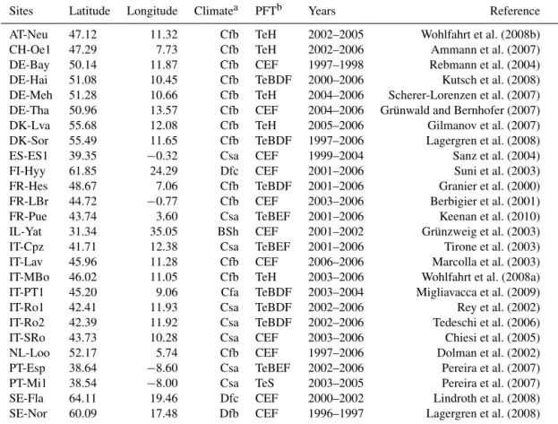
2.4 Modelling protocol and data for site-level simulations
The site-level simulations (single-point simulations) at the FLUXNET sites are run using observed metrological forc-ing, soil properties, and land cover from the La Thuile Dataset (http://fluxnet.fluxdata.org/data/la-thuile-dataset/) of the FLUXNET project (Baldocchi et al., 2001). Data on at-mospheric CO2concentrations are obtained from Sitch et al.
(2015). Reduced and oxidised nitrogen deposition in wet and dry forms and hourly O3 concentrations at 45 m height are
provided by the EMEP model (see Sect. 2.5).
OCN is brought into equilibrium in terms of the terrestrial vegetation and soil carbon and nitrogen pools in a first step with the forcing of the year 1900. In the next step, the model is run with a progressive simulation of the period 1900 up until the start year of the respective site. For this period at-mospheric O3and CO2concentrations as well as N
deposi-tion of the respective simulated years are used. Due to lack of observed climate for the sites for this period, the site-specific observed meteorology from recent years is iterated for these first two steps. The observation years (see Table A1) are sim-ulated with the climate and atmospheric conditions (N depo-sition, CO2and O3concentrations) of the respective years.
For the evaluation of the model output, net ecosystem ex-change (NEE), and latent heat flux (LE), as well as meteoro-logical observations, are obtained for 11 evergreen needle-leaved forest sites, 10 deciduous broadneedle-leaved forest sites, and 5 C3 grassland sites in Europe (see Table A1) from
the La Thuile Dataset of the FLUXNET project (Baldoc-chi et al., 2001). Leaf area indices (LAIs) based on discrete point measurements are obtained from the La Thuile ancil-lary database.
NEE measurements are used to estimate gross primary production (GPP) by the flux-partitioning method accord-ing to (Reichstein et al., 2005). Canopy conductance (Gc)
is derived by inverting the Penman–Monteith equation given the observed LE and atmospheric conditions as described in Knauer et al. (2015).
The half-hourly FLUXNET and model fluxes are filtered prior to deriving average growing-season fluxes (bud break to litter fall) to reduce the effect of model biases on the model-data comparison. Night-time and morning/evening hours are excluded by removing data with lower than 20 % of the daily maximum shortwave downward radiation. To avoid any bi-ases associated with the soil moisture or atmospheric drought response of OCN, we further exclude data points with a mod-elled soil moisture constraint factor (range between 0 and 1) below 0.8 and an atmospheric vapour pressure deficit larger than 0.5 kPa.
Daily mean values are calculated from the remaining time steps only where both modelled and observed values are present. The derived daily values are furthermore constrained to the main growing season by excluding days where the daily GPP is less than 20 % of the yearly maximum daily GPP.
To derive representative diurnal cycles, data for the month July are filtered for daylight hours (taken as incoming short-wave radiation≥100 W m−2), with periods of soil or
atmo-spheric drought stress excluded as above. This is done for modelledFstC,Rc,Vg, andFR and for both modelled and
FLUXNET observed GPP andGc.
2.5 Modelling protocol and data for regional simulations
For the regional simulations, OCN is run at a spatial res-olution of 0.5◦×0.5◦ on a spatial domain focused on
Eu-rope. Daily meteorological forcing (temperature, precipita-tion, shortwave and longwave downward radiaprecipita-tion, atmo-spheric specific humidity, and wind speed) for the years 1961 to 2010 is obtained from RCA3 regional climate model (Samuelsson et al., 2011; Kjellstrom et al., 2011), nested in the ECHAM5 model (Roeckner et al., 2006), and has been bias-corrected for temperatures and precipitation using the CRU climatology (New et al., 1999). Reduced and oxidised nitrogen deposition in wet and dry forms and O3
concentra-tions at 45 m height for the same years are obtained from the EMEP model, which is also run with RCA3 meteorology (as in Simpson et al., 2014b). Emissions for the EMEP runs in current years are as described in Simpson et al. (2014b), and are scaled back to 1900 using data from UNECE and van Aardenne et al. (2001) – see Appendix B. Further details of the EMEP model setup for this grid and meteorology can be found in Simpson et al. (2014b) and Engardt et al. (2017). For OCN, land cover, soil, and N fertiliser application are used as in Zaehle et al. (2011) and kept at 2005 values throughout the simulation. Data on atmospheric CO2concentrations are
ob-tained from Sitch et al. (2015).
iterating the forcing from the period 1961–1970. This is fol-lowed by a simulation for the years 1961–2011 with time-varying climate and atmospheric conditions (N deposition, CO2, and O3concentrations) but with static land cover and
land-use information (kept at year 2005 levels). An upscaled FLUXNET-MTE product of GPP (Jung et al., 2011), us-ing the model tree ensembles (MTE) machine learnus-ing tech-nique, is used to evaluate modelled GPP.
2.6 Impacts of using the ozone deposition scheme In contrast to other terrestrial biosphere models, the OCN ozone module accounts for the effects of aerodynamic, stom-atal and non-stomstom-atal resistance to O3 deposition. Due to
these resistances, the deposition of O3 to leaf level is
re-duced, and the canopy O3 concentration is lower than the
atmospheric O3concentration. Thus, using such a deposition
scheme reduces modelled O3uptake into plants and
accumu-lation. To get an estimate of the magnitude of this impact we compare simulations with the standard deposition scheme as described above (D) with a simulation where O3surface
re-sistance is only determined by stomatal rere-sistance and the non-stomatal depletion of O3is zero (D-STO), as well as a
further simulation where no deposition scheme is used and the canopy O3concentration is equal to the atmospheric
con-centration (ATM).
3 Results
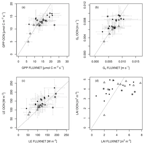
3.1 Evaluation against daily eddy-covariance data Figure 1 a shows that, for most sites, modelled and observation-based GPP agree well (see Table A2 for R2
and RMSE values). The standard deviation is larger for the observation-based estimates because of the high level of noise in the eddy-covariance data. For sites dominated by needle-leaved trees, the modelled and observation-based GPP values are very close, with only slight under- and over-estimates by the model at some sites. At sites dominated by broadleaved trees, modelled GPP deviates more strongly from the observation-based GPP, underestimating the obser-vations in 7 out of 10 cases. However, the results are within the range of standard deviation except for the drought-prone PT-Mi1 site (see Fig. A1a for an explicit site comparison). At C3grassland sites, modelled GPP is in good agreement with
the observation-based GPP except for AT-Neu, which has the highest mean GPP of all sites observed by FLUXNET with a large standard deviation, which may reflect the effect of site management (e.g. mowing and fertilisation), for which no data were readily available as model forcing.
When comparing modelled and observed latent heat flux (LE), the model fits the observations best at the needle-leaved forest sites (Fig. 1c). However, LE is overestimated at 9 out of 10 broadleaved forest sites but remains within the range of the large observational standard deviation. At sites
dom-inated by C3 grasses the modelled LE differs considerably
from the observed value, at two sites overestimating and two underestimating the fluxes, again within the observational standard deviation.
In agreement with the comparison of GPP and LE, the comparison of modelled to observation-based canopy con-ductance (Gc) shows the best agreement for sites
domi-nated by needle-leaved trees (Fig. 1b). At sites domidomi-nated by broadleaved trees, the modelledGcvaries more widely from
the FLUXNETGc. The modelledGc at sites dominated by
C3grasses is in very good agreement with FLUXNET Gc,
with slight overestimation of Gc at two out of three sites,
except for the DE-Meh site, where means differ outside the standard deviation (see Fig. A1b).
The comparison of the average modelled summertime LAI and point measurements at the FLUXNET illustrates that the variability in the measured LAI is much greater than that of OCN (Fig. 1d). The modelled LAI values approach light-saturating, maximum LAI values and are not able to repro-duce between-site differences in, for example, the growth stage, site history, or maximum possible LAI values. Fur-thermore, it should be borne in mind that the observed LAI values are averages of point measurements, which are not necessarily representative of the modelled time period, and that the model had not been parameterised specifically for the sites. Modelled GPP depends not only on LAI but also on light availability, temperature, and soil moisture. The much better represented values of GPP,Gc, and LE compared to
FLUXNET data (Fig. 1a–c) indicate that OCN is able to ad-equately transform available energy into carbon uptake and water loss and thus simulate key variables impacting ozone uptake within a reasonable range.
3.2 Mean diurnal cycles of key O3parameters.
For further evaluation of the modelled O3uptake, we
anal-ysed the diurnal cycles of O3uptake (FstC), O3surface
re-sistance (Rc), O3 deposition velocity (Vg), and flux ratio
(FR)) as well as GPP and Gc. We selected three sites (a
broadleaved, a needle-leaved, and a C3 grass site) based on
the selection criteria that modelled and FLUXNET GPP and LAI agree well and a minimum of five observation years is available to reduce possible biases from the inability of the model to simulate short-term variations from the mean. The selected sites are a temperate broadleaved summer green forest (IT-Ro1), a boreal needle-leaved evergreen forest (FI-Hyy), and a temperate C3 grass land (CH-Oe1). We
eval-uate modelled GPP and Gc against observations from the
FLUXNET sites. The modelled mean diurnal cycles of O3
related variables (FstC,Rc,Vg,FR) are compared to reported
values in the literature since we did not have access to site-specific observations.
Modelled and observed mean diurnal cycles of GPP and
Gcare in general agreement at the three selected FLUXNET
0 5 10 15 20 25 30
0
5
10
15
20
GPP FLUXNET [µmol C m−2 s−1]
GPP OCN [
µ
mol C m
−
2 s
−
1]
(a)
0.000 0.005 0.010 0.015
0.000
0.004
0.008
0.01
2
Gc FLUXNET [m s− 1
] Gc
OCN [m s
−
1]
(b)
0 50 100 150 200 250
0
50
100
150
200
250
LE FLUXNET [W m−2]
LE OCN [W m
−
2]
(c)
0 2 4 6 8
012345
LAI FLUXNET [m2 m−2]
LAI OCN [m
2 m
−
2]
(d)
Figure 1.Comparison of measured(a)GPP,(b)canopy conductance (Gc),(c)latent heat flux (LE), and(d)LAI at 26 European FLUXNET sites and simulations by OCN. Displayed are means and standard deviations of daily means of the measuring/simulation period, with the exception of FLUXNET-derived LAI, which is based on point measurements. Dots symbolise sites dominated by broadleaved trees, triangles sites dominated by needle-leaved trees, and asterisks sites dominated by C3grasses. The grey line constitutes the 1:1 line.
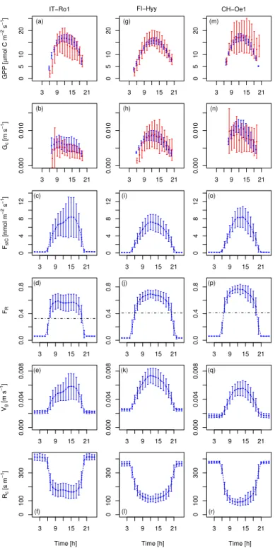
agreement for the mean diurnal cycle of GPP at the needle-leaved site FI-Hyy, where the hourly means are very close and the observational standard deviation is narrow (see Fig. 2g). At the grassland site IT-Ro1 the overall daytime magnitude of the fluxes is reproduced in general except for the observed afternoon reduction in GPP (see Fig. 2a). The modelled hourly values fall in the range of the observed val-ues. Modelled and observation-based hourly means of GPP at the site CH-Oe1 agree well except for the evening hours, where the observed values increase again. The mean diur-nal cycles ofGcderived from the FLUXNET data are again
best matched at the site FI-Hyy, whereas the model gener-ally overestimates the diurnal cycle ofGcslightly at the site
IT-Ro1, and overestimates peakGcat the CH-Oe1 site. The
fact that OCN does not always simulate the observed midday depression of Gc, suggests that the response of stomata to
atmospheric and soil drought in OCN requires further eval-uation and improvement. Similar to the daily mean values (see Fig. 1a, b), the mean hourly values show the best match of GPP and Gc for the needle-leaved tree site and stronger
deviations for the sites covered by broadleaved trees and C3
grasses.
The stomatal O3 uptake FstC (Fig. 2c, i, o) is close to
zero during night-time, when the stomata are assumed to be closed, because gross photosynthesis is zero. At FI-Hyy and CH-Oe1, peak uptake occurred at noon, when photosynthesis (Fig. 2g, m) and stomatal conductance (Fig. 2h, n) are high-est, at values between 8 and 9 nmol m−2s−1. At the Italian
site IT-Ro1, maximum uptake occurs in the afternoon hours around 15 h, with much larger standard deviation compared to the other two sites (Fig. 2c). The magnitude of stomatal O3uptake corresponds well to some values reported, for
ex-ample, for crops (Gerosa et al., 2003, 2004; daily maxima of 4–9 nmol m−2s−1) and holm oak (Vitale et al., 2005; approx.
7–8 nmol m−2s−1). Lower daily maximum values have been
reported for an evergreen Mediterranean forest dominated by Holm Oak of 4 nmol m−2s−1under dry weather conditions
(Gerosa et al., 2005) and 1–6 nmol m−2s−1for diverse
south-ern European vegetation types (Cieslik, 2004). Much higher values are reported forPicea abies (50–90 nmol m−2s−1), Pinus cembra(10–50 nmol m−2s−1), andLarix decidua(10–
40 nmol m−2s−1) at a site near Innsbruck, Austria (Wieser
et al., 2003), where canopy O3uptake was estimated by
be-3 9 15 21
0
5
10
20
GPP [
µ
mol C m
−
2 s
−
1] (a) IT−Ro1
3 9 15 21
0.000
0.010
Gc
[m s
−
1]
(b)
3 9 15 21
048
1
2
FstC
[nmol m
−2
s
−1
] (c)
3 9 15 21
0.0
0.4
0.8
FR (d)
3 9 15 21
0.000
0.004
0.008
Vg
[m s
−
1]
(e)
3 9 15 21
0
100
300
Time [h] Rc
[s m
−
1]
(f)
3 9 15 21
0
5
10
20
(g) FI−Hyy
3 9 15 21
0.000
0.010
(h)
3 9 15 21
048
1
2 (i)
3 9 15 21
0.0
0.4
0.8
(j)
3 9 15 21
0.000
0.004
0.008
(k)
3 9 15 21
0
100
300
Time [h] (l)
3 9 15 21
0
5
10
20
(m) CH−Oe1
3 9 15 21
0.000
0.010
(n)
3 9 15 21
048
1
2 (o)
3 9 15 21
0.0
0.4
0.8
(p)
3 9 15 21
0.000
0.004
0.008
(q)
3 9 15 21
0
100
300
Time [h] (r)
Figure 2.Simulated and observed hourly means over all days of the months of July of 2002–2006 for CH-Oe1 and IT-Ro1, as well as for 2001–2006 for FI-Hyy. Plotted are mean hourly values (local time) of(a, g, m)GPP (blue: OCN; red: FLUXNET),(b, h, n)canopy conductance (Gc) (blue: OCN; red: FLUXNET),(c, i, o)O3uptake (FstC),(d, j, p)the flux ratio (FR),(e, k, q)O3deposition velocity (Vg),
and(f, l, r)O3surface resistance (Rc). The error bars indicate the standard deviation from the hourly mean. The dotted line in panels(d),
(j), and(p)indicates the daily mean value.
fore where the eddy-covariance technique was applied. The much higher FstC values in that study result from much
higher canopy conductances to O3 (GOc3), which are up to
12 times higher than the modelled GOc3 values in our study
(see Fig. 2,GOc3=1G.51c ).
The ratio between the stomatal O3uptake and the total
sur-face uptake (FR) is close to zero during night-time hours and
are close to 0.6 at IT-Ro1, around 0.7 at FI-Hyy, and close to 0.8 at CH-Oe1. These values are comparable to the ra-tios reported for crops (Gerosa et al., 2004; Fowler et al., 2009; 0.5–0.6), Norway spruce (Mikkelsen et al., 2004; 0.3– 0.33), and various southern European vegetation types (Cies-lik, 2004; 0.12–0.69). The modelled flux ratios here show slightly higher daily maximum flux ratios than reported in the listed studies. Daily mean flux ratios are well within the reported range.
The modelled deposition velocities Vg are lowest
dur-ing night-time, with values of approximately 0.002 m s−1
(Fig. 2e, k, q). These values increase to maximum hourly means of 0.006–0.007 m s−1 during daytime. These values
compare well with reported values of deposition velocities, which range from 0.003 to 0.009 m s−1at noon (Gerosa et al.,
2004) for a barley field and are approximately 0.006 m s−1
at noon for a wheat field (Tuovinen et al., 2004) and ap-proximately 0.009 m s−1 at noon at a potato field (Coyle
et al., 2009). The estimates for FI-Hyy also agree well with maximum deposition velocities reported for Scots pine site of 0.006 m s−1 (Keronen et al., 2003; Tuovinen et al.,
2004) and noon values from Danish Norway spruce sites of 0.006–0.010 m s−1(Mikkelsen et al., 2004; Tuovinen et al.,
2001). Mean daytime deposition velocities of 0.006 m s−1
(range 0.003–0.008 m s−1) are reported at a Finnish
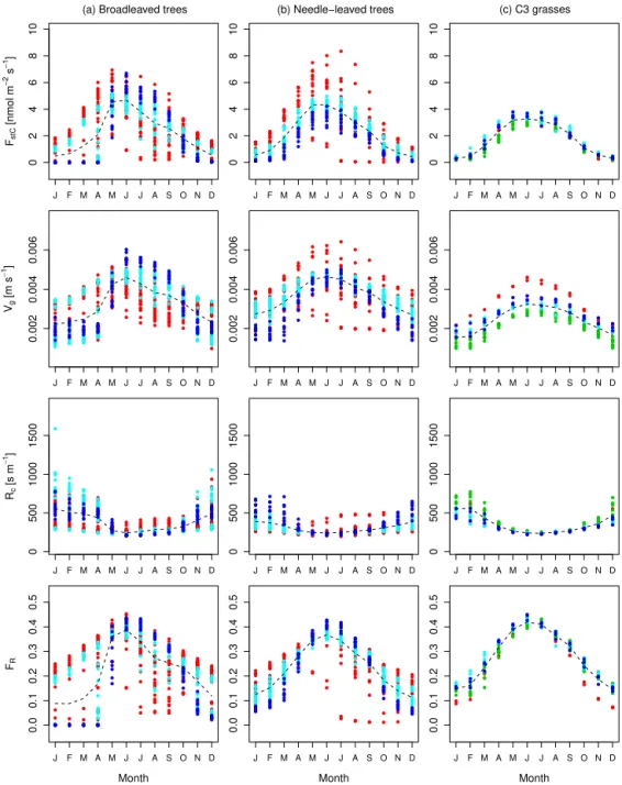
moun-tain birch site (Tuovinen et al., 2001). Simulated monthly mean values ofVgdiffer substantially between the sites (see
Fig. A2). When comparing the monthly means over all sites (Fig. A2 dashed line) of a functional group (broadleaved, needle-leaved, C3grasses) to the ensemble mean of 15 CTMs
(Hardacre et al., 2015), the values simulated here are higher for needle-leaved tree sites. For broadleaved tree sites and grassland sites, higher values, but which are still within the observed ensemble range, are found for the summer months. The modelled hourly mean O3 surface resistance Rc is
highest during night-time, at approximately 400 s m−1, and
decreases during daytime to values of 100–180 s m−1, where
the lowest surface resistance of approximately 100 s m−1is
modelled at the grassland site CH-Oe1 (Fig. 2f, l, r). These values are slightly higher than independent estimates (for grasses and crops obtained for other sites) of noon surface re-sistances ranging from 50 to 100 s m−1(Padro, 1996; Coyle
et al., 2009; Gerosa et al., 2004; Tuovinen et al., 2004). Tuovinen et al. (2004) reported noon values of approximately 140 sm−1for a Scots pine forest and 70–140 s m−1for a
Nor-way spruce forest site (Tuovinen et al., 2001), which com-pares well with the modelledRcvalues at the needle-leaved
forest site (FI-Hyy; Fig. 2l). Higher noon values of approx-imately 250 s m−1are reported at a Danish Norway spruce
site (Mikkelsen et al., 2004). For a mountain birch forest, noon values of 110–140 s m−1(Tuovinen et al., 2001) are
ob-served which is slightly lower than the modelled value at the IT-Ro1 site (dominated by broadleaved tree PFT).
Ra b rext R ^
gs Gc Rb
−1.0
−0.5
0.0
0.5
1.0 (a)
Ra b rext R ^
gs Gc Rb
FR Fg FstC Vg Rc
0.0
0.2
0.4
0.6
0.8
1.0 (b)
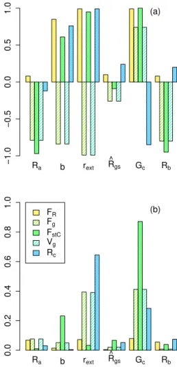
Figure 3. (a)Mean partial correlation coefficients and(b)strength of the correlation in % per %.Ra,b,rext,Rˆgs, andGcare perturbed
within±20 % of their central estimate. Results from simulations at the FLUXNET site FI-Hyy for the simulation period 2001–2006.
3.3 Sensitivity analysis
We assess the sensitivity of the modelled O3uptake and
de-position, represented byFg,FstC,Vg, andRc, to uncertainty
in six weakly constrained variables and parameters of the O3
deposition scheme (Ra,b,rext,Rˆgs,Gc, andRb). Figure 3a
shows, for example, the results for the boreal needle-leaved forest FI-Hyy. As expected, all uptake/deposition variables, except for the flux ratio (FR) are negatively correlated with
the aerodynamic resistanceRa, which describes the level of
decoupling of the atmosphere and land surface. Increasing
Radecreases the canopy internal O3concentration and hence
stomatal (FstC) and total (Fg) deposition as well as the
depo-sition velocity (Vg). The flux ratioFR is slightly positively
correlated with changes inRa due to the stronger negative
correlation ofFstCrelative toFg.
In decreasing order, but as expected, the level of external leaf resistance (rext), the scaling factorb(Eq. 9), the soil
re-1 57 113 169 225 281 337
0246
FstC
[nmol m
−
2 s
−
1 ] (a)
1 57 113 169 225 281 337
0.1
0.3
0.5
FR (b)
1 57 113 169 225 281 337
0.001
0.004
Vg
[m s
−
1 ]
(c)
1 57 113 169 225 281 337
200
600
Rc
[s m
−
1 ]
(d)
1 57 113 169 225 281 337
10
30
50
O3
[ppb]
(e)
Time [d]
130
140
150
160
CUO [mmol m
−
2 ]
0.000
0.003
Gc
[m s
−
1 ]
Time [d]
1 57 113 169 225 281 337
(f)
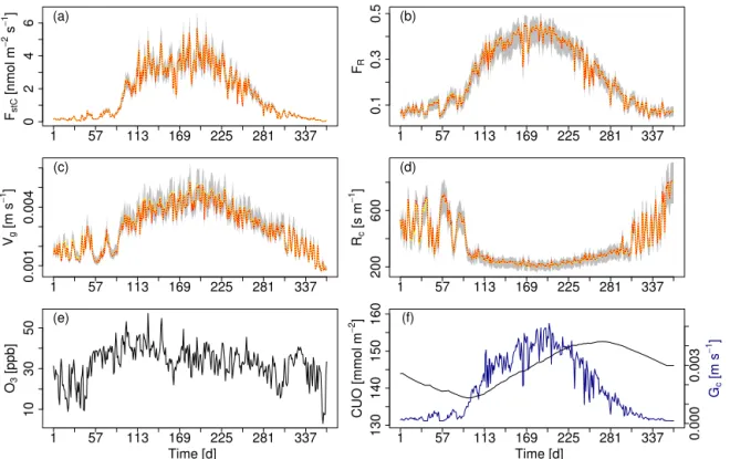
Figure 4.Ensemble range of key O3uptake/deposition variables resulting from the perturbation ofRa,b,rext,Rˆgs, andGcwithin±20 % of their central estimate. Shown are simulated daily mean values of(a)O3uptake (FstC),(b)the O3flux ratio (FR),(c)O3deposition velocity (vg) and(d)O3surface resistance (Rc) for the boreal needle-leaved evergreen forest at the finish FLUXNET site FI-Hyy for the year 2001. Red dashed: unperturbed model; yellow: median of all sensitivity runs; light-grey area: min–max range of all sensitivity runs. Simulated daily mean values for the respective site and year of(e)atmospheric O3concentrations O3and(f)cumulative uptake of O3(CUO) and canopy
conductanceGc.
sistance (Rb) increase Rc and consequently reduce Fg and
Vg. Reducing the non-stomatal deposition by increasingrext,
b,Rˆgs, andRbincreases the canopy internal O3
concentra-tion and thus stomatal O3 uptake (FstC). The combined
ef-fects of a reduction in total depositionFgand an increase in
FstCcause a positive correlation ofFRtorext,b,Rˆgs, andRb.
Increasing canopy conductance (Gc) increases stomatal
O3uptake (FstC) and thereby also increasesVgandFg. The
increased total O3 uptake (Fg) decreases the surface
resis-tance to O3uptakeRc, resulting in a negative correlation of
RcwithGc. The stronger increase inFstC relative toFg
re-sults in a positive correlation ofFR.
Despite these partial correlations, only changed values for
rext and Gc have a notable effect on the predicted fluxes
(Fig. 3b), whereas for the other factors (Ra,b, andRˆgs) the
impact on the simulated fluxes is less than 0.1 % due to a 1 % change in the variables/parameters of the deposition scheme. The flux ratioFRis very little affected by varyingrextand
Gc.
Notwithstanding the perturbations, all four O3related flux
variables show a fairly narrow range of simulated values (Fig. 4). For all four variables the unperturbed model and the ensemble mean lie on top of each other (see dashed red and
yellow line in Fig. 4a–d). The seasonal course of the surface resistances and fluxes is maintained. The simulations show a strong day-to-day variability inFstC, which is conserved with
different parameter combinations and which is largely driven by the day-to-day variations inGc and the atmospheric O3
concentration (see Fig. 4f and e respectively). Ozone uptake by the leaves reduces the O3 surface resistance during the
growing season such thatRc becomes lowest. The
cumula-tive uptake of O3 (CUO) is lowest at the beginning of the
growing season but not zero because the evergreen pine at the Hyytiälä site accumulates O3over several years (Fig. 4f).
The CUO increases during the growing season and declines in autumn, when a larger fraction of old needles are shed.
The minor impact of the perturbations on the simulated O3
uptake and deposition variables suggests that the calculated O3uptake is relatively robust against uncertainties in the
pa-rameterisation of some of the lesser known surface proper-ties.
3.4 Regional simulations
produc-tion over Europe for the period 2001–2010 (see Sect. 2.5 for modelling protocol).
Simulated mean annual GPP for the years 1982–2011 shows in general good agreement with an independent es-timate of GPP based on upscaled eddy-covariance measure-ments (MTE; see Sect. 2.5), with OCN on average underesti-mating GPP by 16 % (European mean). A significant excep-tion are cropland dominated areas (Fig. 5) in parts of eastern Europe, southern Russia, Turkey, and northern Spain, which show consistent overestimation of GPP by OCN of 400– 900 g C m−2yr−1(58 % overestimation on average). Regions
with a strong disagreement coincide with high simulated LAI values by OCN and a higher simulated GPP in summer com-pared to the summer GPP by MTE. In addition, OCN sim-ulates a longer growing season for croplands since sowing and harvest dates are not considered. It is worth noting, nev-ertheless, that there are no FLUXNET stations present in the regions of disagreement hotspots, making it difficult to assess the reliability of the MTE product in this region.
North of 60◦N, OCN has the tendency to produce
lower estimates of GPP than inferred from the observation-based product, which is particularly pronounced in low-productivity mountain regions of Norway and Sweden. It is unclear whether this bias is indicative of a N limitation that is too strong in the OCN model.
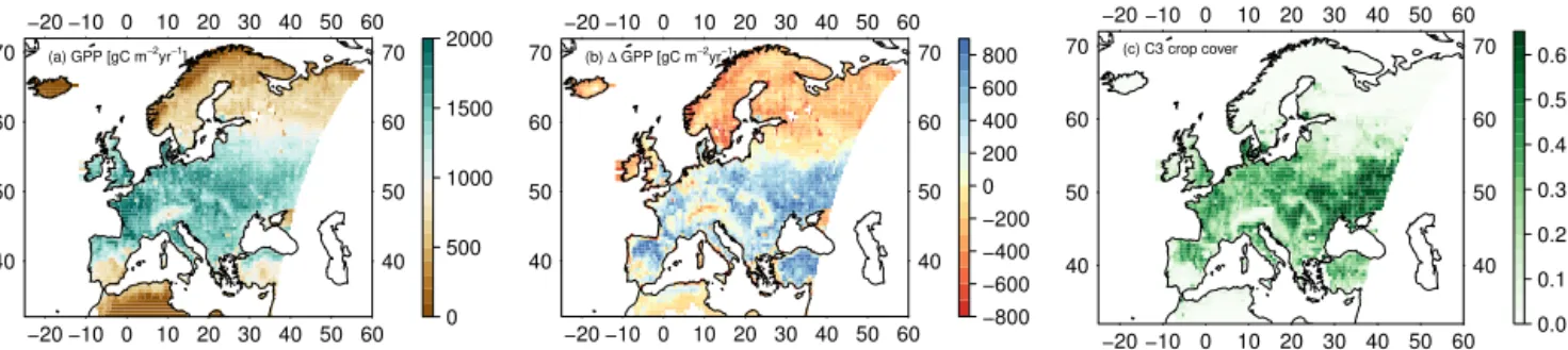
Average decadal O3 concentrations generally increase
from northern to southern Europe (Fig. 6a) and with in-creasing altitude, with local deviations from this pattern in centres of substantial air pollution. The pattern of foliar O3 uptake differs distinctly from that of the O3
concentra-tions, showing highest uptake rates in central and eastern Europe and parts of southern Europe (Fig. 6b), associated with centres of high rates of simulated gross primary pro-duction (Fig. 5a) and thus canopy conductance. The cumu-lative O3uptake reaches values of 40–60 mmol m−2in large
parts of central Europe (Fig. 6c). The highest accumulation rates of 80–110 mmol m−2are found in eastern Europe and
parts of Scandinavia as well as in Italy, the Alps, and the Bordeaux region. The concentration-based exposure index AOT40 (Fig. 6d) shows a strong north–south gradient similar to the O3concentration (Fig. 6a) and is distinctly different to
the flux-based CUO pattern (Fig. 6c).
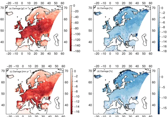
Simulated reduction in mean decadal GPP due to O3range
from 80 to 160 g C m−2yr−1over large areas of central,
east-ern, and south-eastern Europe (Fig. 7a) and is generally largest in regions of high productivity. The relative reduc-tion in GPP is fairly consistent across large areas in Europe and averages 6–10 % (Fig. 7b). Higher reductions in relative terms are found in regions with high cover of C4PFTs, e.g.
the Black Sea area. Lower relative reductions are found in northern Europe and parts of southern Europe, where pro-ductivity is low and stomatal O3 uptake is reduced by, for
example, low O3concentrations or drought control on
stom-atal fluxes respectively. Slight increases or strong decreases in relative terms are found in regions with very small
produc-tivity like in northern Africa and the mountainous regions of Scandinavia. A slight increase in GPP might be caused by feedbacks of GPP damage on LAI, canopy conductance, and soil moisture content such that water savings, for example, enable a prolonged growing season and thus a slightly higher GPP. Overall, simulated European productivity has been re-duced from 10.6 to 9.8 Pg C yr−1 corresponding to a 7.6 %
reduction.
The O3-induced reductions in GPP are associated with
a reduction in mean decadal transpiration rates of 8– 15 mm yr−1 over large parts of central and eastern Europe
(Fig. 7c). These reductions correspond to 3–6 % of transpira-tion in central Europe and 6–10 % in northern Europe. As ex-pected, the relative reductions in transpiration rates are there-fore slightly less than for GPP due to the role of aerodynamic resistance in controlling water fluxes in addition to canopy conductance. Very high reductions in transpiration are found in the eastern Black Sea area associated with strong reduc-tions in GPP and in the mountainous regions of Scandinavia, where absolute changes in transpiration are very small. Re-gionally (in particular in eastern Spain, northern Africa, and around the Black Sea) lower reductions in transpiration or even slight increases are found (Fig. 7d). These are related to O3-induced soil moisture savings during the wet growing
season, leading to lower water stress rates during the drier season. The very strong reduction in transpiration west of the Crimean Peninsula are related to the strong reductions in GPP mentioned above. Overall, simulated European mean transpiration has been reduced from 170.4 to 163.3 mm cor-responding to a 4.2 % reduction.
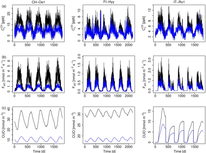
3.5 Impacts of using the ozone deposition scheme At the FI-Hyy site the canopy O3 concentration, uptake
and accumulated uptake (CUO) increases approximately 10– 15 % for the D-STO model (non-stomatal depletion of O3
is zero) and 20–25 % for the ATM model version (canopy O3concentration is equal to the atmospheric concentration)
compared to the standard deposition scheme (D) used here (Figs. 8a–c and A3). The exact values however are site- and PFT-specific (see Fig. A3 for the CH-Oe1 and IT-Ro1 site).
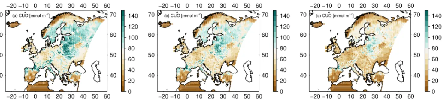
The regional impact of using the ozone deposition scheme on CUO is shown in Fig. 9. CUO substantially decreases for the D-STO (Fig. 9b) compared to the ATM model (Fig. 9a). Using the standard deposition model D (Fig. 9c) further re-duces the CUO compared to the ATM version where the stomata respond directly to the atmospheric O3
concentra-tion.
Calculating the canopy O3 concentration with the help
of a deposition scheme that accounts for stomatal and non-stomatal O3deposition thus reduces O3accumulation in the
−20 −10 0 10 20 30 40 50 60
40 50 60 70
−20 −10 0 10 20 30 40 50 60 40 50 60 70
0 500 1000 1500 2000 (a) GPP [gC m−2yr−1]
−20 −10 0 10 20 30 40 50 60
40 50 60 70
−20 −10 0 10 20 30 40 50 60 40 50 60 70
−800 −600 −400 −200 0 200 400 600 800 (b) Δ GPP [gC m−2yr−1]
−20 −10 0 10 20 30 40 50 60
40 50 60 70
−20 −10 0 10 20 30 40 50 60 40 50 60 70
0.0 0.1 0.2 0.3 0.4 0.5 0.6 (c) C3 crop cover
Figure 5.Europe-wide simulated GPP and difference between modelled GPP by OCN and a GPP estimate by a FLUXNET-MTE product. Plotted, for the years 1982–2011, are(a)the simulated mean GPP accounting for ozone damage in g C m−2yr−1,(b)the mean differences for OCN minus MTE GPP in g C m−2yr−1, and(c)the mean simulated grid cell cover of the C3-crop PFT in OCN, given as fractions of the
total grid cell area.
−20 −10 0 10 20 30 40 50 60
40 50 60 70
−20 −10 0 10 20 30 40 50 60
40 50 60 70
30 35 40 45 50 (a) O3 [ppb]
−20 −10 0 10 20 30 40 50 60
40 50 60 70
−20 −10 0 10 20 30 40 50 60
40 50 60 70
0.0 0.5 1.0 1.5 2.0 (b) FstC [nmol m−2s−1]
−20 −10 0 10 20 30 40 50 60
40 50 60 70
−20 −10 0 10 20 30 40 50 60
40 50 60 70
0 20 40 60 80 100 (c) CUO [mmol m−2]
−20 −10 0 10 20 30 40 50 60
40 50 60 70
−20 −10 0 10 20 30 40 50 60
40 50 60 70
0 5000 10 000 15 000 20 000 25 000 30 000 35 000 (d) AOT40 [ppb yr−1]
Figure 6.Mean decadal(a)O3concentration (ppb),(b)canopy-integrated O3uptake into the leaves (nmol m−2s−1),(c)canopy-integrated cumulative uptake of O3(CUO) (mmol m−2), and(d)AOT40 (ppm yr−1), for Europe of the years 2001–2010.
4 Discussion
We extended the terrestrial biosphere model OCN by a scheme to account for the atmosphere–leaf transfer of O3in
order to better account for air pollution effects on net pho-tosynthesis and hence regional to global water, carbon, and nitrogen cycling. This ozone deposition scheme calculates canopy O3concentrations and uptake into the leaves
depend-ing on surface conditions and vegetation carbon uptake Estimates of the regional damage to annual average GPP (−7.6 %) and transpiration (−4.2 %) simulated by OCN for 2001–2010 are lower than previously reported estimates. Meta-analyses suggest on average a 11 % (Wittig et al., 2007)
and a 21 % (Lombardozzi et al., 2013) reduction in instanta-neous photosynthetic rates. However, because of carry-over effects, this does not necessarily translate directly into reduc-tions in annual GPP. Damage estimates using the CLM sug-gest GPP reductions of 10–25 % in Europe and 10.8 % glob-ally (Lombardozzi et al., 2015). Reductions in transpiration have been estimated as 5–20 % for Europe and 2.2 % glob-ally (Lombardozzi et al., 2015). Lombardozzi et al. (2015), however, used fixed reductions of photosynthesis (12–20 %) independent of cumulative O3 uptake for two out of three
simulated plant types. Damage was only related to cumula-tive O3 uptake for one plant type with a very small slope
cu-−20 −10 0 10 20 30 40 50 60
40 50 60 70
−20 −10 0 10 20 30 40 50 60
40 50 60 70
−160 −140 −120 −100 −80 −60 −40 −20 0 (a) Damage [gC m−2yr ]−1
−20 −10 0 10 20 30 40 50 60
40 50 60 70
−20 −10 0 10 20 30 40 50 60
40 50 60 70
−18 −16 −14 −12 −10 −8 −6 −4 −2 0 (b) Damage [%]
−20 −10 0 10 20 30 40 50 60
40 50 60 70
−20 −10 0 10 20 30 40 50 60
40 50 60 70
−16 −14 −12 −10 −8 −6 −4 −2 0 (c) Damage [mm yr−1]
−20 −10 0 10 20 30 40 50 60
40 50 60 70
−20 −10 0 10 20 30 40 50 60
40 50 60 70
−15 −10 −5 0 (d) Damage [%]
Figure 7.Mean decadal(a)reduction in GPP (g C m−2yr−1),(b)percent reduction in GPP,(c)reduction in transpiration (mm yr−1), and (d)percent reduction in transpiration due to ozone damage averaged for the years 2001–2010.
0 500 1000 1500 2000
10
20
30
40
50
Time [d] Cc
O3
[ppb]
(a)
0 500 1000 1500 2000
02468
Time [d] FstC
[nmol m
−
2 s
−
1]
(b)
0 500 1000 1500 2000
140
160
180
Time [d]
CUO [mmol m
−
2 ]
(c)
Figure 8.Mean daily values of the(a)O3surface concentration (ppb),(b)canopy-integrated O3uptake into the leaves (nmol m−2s−1), and
(c)canopy-integrated cumulative uptake of O3(CUO) (mmol m−2) at the FLUXNET site FI-Hyy. Black: ATM model; dark blue: D-STO model; light blue: standard deposition model (D).
mulative O3uptake. Sitch et al. (2007) simulated global GPP
reductions of 8–14 % (under elevated and fixed CO2
respec-tively) for low plant ozone sensitivity and 15–23 % (under elevated and fixed CO2 respectively) for high plant ozone
sensitivity for the year 2100 compared to 1901. For the Euro-Mediterranean region an average GPP reduction of 22 % was estimated by the ORCHIDEE model for the year 2002 using an AOT40-based approach (Anav et al., 2011).
Possible causes for the discrepancies are differences in dose–response relationships, flux thresholds accounting for the detoxification ability of the plants, atmospheric O3
con-centrations, simulation periods, and simulation of climate
change (elevated CO2) and air pollution (nitrogen
deposi-tion). We discuss the most important aspects below. To elu-cidate the reasons for the substantial differences in the dam-age estimates, further studies are necessary to disentangle the combined effects of differing flux thresholds, damage rela-tionships, climate change, and deposition of nitrogen.
4.1 Atmosphere–leaf transport of ozone
The sensitivity analysis in Sect. 3.3 demonstrates that the es-timate of canopy conductance (Gc) is crucial for
−20 −10 0 10 20 30 40 50 60
40 50 60 70
−20 −10 0 10 20 30 40 50 60 40 50 60 70
0 20 40 60 80 100 120 140 (a) CUO [mmol m−2]
−20 −10 0 10 20 30 40 50 60
40 50 60 70
−20 −10 0 10 20 30 40 50 60 40 50 60 70
0 20 40 60 80 100 120 140 (b) CUO [mmol m−2]
−20 −10 0 10 20 30 40 50 60
40 50 60 70
−20 −10 0 10 20 30 40 50 60 40 50 60 70
0 20 40 60 80 100 120 140 (c) CUO [mmol m−2]
Figure 9.Mean decadal canopy-integrated cumulative uptake of O3(CUO) (mmol m−2) for Europe of the years 2001–2010.(a)Canopy O3concentration is equal to the atmospheric concentration (ATM) and(b)O3surface resistance is only determined by stomatal resistance (D-STO).(c)Standard ozone deposition scheme (D).
constrain modelled canopy conductance are highly impor-tant. The site-level evaluation shows that OCN produces rea-sonable estimates of simulated gross primary productivity (GPP), canopy conductance, and latent heat flux (LE) com-pared to FLUXNET observations. This agreement has to be seen in the light of the diverse set of random and system-atic errors in the eddy-covariance measurements as well as derived flux and conductance estimates (Richardson et al., 2012; Knauer et al., 2016). Next to uncertainties about the strength of the aerodynamic coupling between atmosphere and canopy, problems exist at many sites with respect to the energy balance closure (Wilson et al., 2002). Failure to close the energy balance can cause underestimation of sen-sible and latent heat, as well as an overestimation of avail-able energy, with mean bias of 20 % where the imbalance is greatest during nocturnal periods (Wilson et al., 2002). This imbalance propagates to estimates of canopy conductance, which is inferred from latent and sensible heat fluxes. The energy imbalance furthermore appears to affect estimates of CO2uptake and respiration (Wilson et al., 2002). Flux
par-titioning algorithms which extrapolate night-time ecosystem respiration estimates to daytime introduce an additional po-tential for bias in the estimation of GPP (Reichstein et al., 2005). Nevertheless, the general good agreement ofGc
com-pared to FLUXNET estimates, together with the finding that modelled values of key ozone variables are within observed ranges, supports the use of the extended OCN model for de-termining the effect of air pollution on terrestrial carbon, ni-trogen, and water cycling.
A key difference from previous studies is our use of the use of the ozone deposition scheme, which reduces O3
sur-face concentrations and hence also the estimated O3uptake
and accumulation (see Fig. 9). Accounting for stomatal and non-stomatal deposition in the calculation of the surface O3
concentrations considerably impacts the estimated plant up-take of O3. O3 uptake and cumulated uptake are
consider-ably overestimated when atmospheric ozone concentrations are used to calculate O3 uptake or when in the calculation
of leaf-level O3concentrations only stomatal destruction of
O3 is regarded (see Sect. 3.5). Compared to the values that
would have been obtained if the CTM O3concentrations of
the atmosphere (from ca. 45 m height) had been used di-rectly at the leaf surface, our simulations yield a decrease in CUO by 31 % (European means for the years 2001–2010). A significant fraction of the decreases is associated with non-stomatal O3 uptake and destruction at the surface, which
decreased the simulated cumulative O3 uptake by 16 %. To
obtain an estimate of CUO that is as accurate as possible, stomatal and non-stomatal destruction of O3 and their
im-pacts on canopy O3concentrations should be accounted for
in terrestrial biosphere models (Tuovinen et al., 2009). Flux-based ozone damage assessment models may overestimate ozone-related damage unless they properly account for non-stomatal O3uptake at the surface.
We note that vegetation type and dynamics also impact the stomatal and non-stomatal deposition of O3, and hence
the calculation of the leaf-level O3concentrations. This
im-pedes the use of CTM-derived leaf-level O3 concentration,
as CTM and vegetation specifications may differ strongly. Using the O3 from the lowest level of the atmosphere
re-duces this problem, but running a terrestrial biosphere with a fixed atmospheric boundary condition (and not coupled to a atmospheric CTM) is still a simplification that prevents biosphere–atmosphere feedbacks and therefore to potential discrepancies between vegetation and CTM. Not accounting for this feedback and stomatal and non-stomatal O3
depo-sition might result in an overestimation of O3 uptake and
hence potential damage in the vegetation model. The deposi-tion scheme in OCN offers the potential to couple vegetadeposi-tion and chemical transport modelling and is thus a step forward towards coupled atmosphere–vegetation simulations.
4.2 Estimating vegetation damage from ozone uptake A key aspect of ozone damage estimates are the assumed dose–response relationships, which relate O3 uptake to