of Canopy Density and Light Environment: A Model for
Amphibolis griffithii
John D. Hedley1*, Kathryn McMahon2, Peter Fearns3
1Environmental Computer Science Ltd., Tiverton, Devon, United Kingdom,2School of Natural Sciences and Centre for Marine Ecosystems Research, Edith Cowan University, Joondalup, Western Australia,3Department of Imaging and Applied Physics, Curtin University of Technology, Perth, Western Australia
Abstract
A three-dimensional computer model of canopies of the seagrass Amphibolis griffithii was used to investigate the consequences of variations in canopy structure and benthic light environment on leaf-level photosynthetic saturation state. The model was constructed using empirical data of plant morphometrics from a previously conducted shading experiment and validated well toin-situdata on light attenuation in canopies of different densities. Using published values of the leaf-level saturating irradiance for photosynthesis, results show that the interaction of canopy density and canopy-scale photosynthetic response is complex and non-linear, due to the combination of self-shading and the non-linearity of photosynthesis versus irradiance (P-I) curves near saturating irradiance. Therefore studies of light limitation in seagrasses should consider variation in canopy structure and density. Based on empirical work, we propose a number of possible measures for canopy scale photosynthetic response that can be plotted to yield isoclines in the space of canopy density and light environment. These plots can be used to interpret the significance of canopy changes induced as a response to decreases in the benthic light environment: in some cases canopy thinning can lead to an equivalent leaf level light environment, in others physiological changes may also be required but these alone may be inadequate for canopy survival. By providing insight to these processes the methods developed here could be a valuable management tool for seagrass conservation during dredging or other coastal developments.
Citation:Hedley JD, McMahon K, Fearns P (2014) Seagrass Canopy Photosynthetic Response Is a Function of Canopy Density and Light Environment: A Model for Amphibolis griffithii. PLoS ONE 9(10): e111454. doi:10.1371/journal.pone.0111454
Editor:Kay C. Vopel, Auckland University of Technology, New Zealand
ReceivedJune 19, 2014;AcceptedOctober 2, 2014;PublishedOctober 27, 2014
Copyright:ß2014 Hedley et al. This is an open-access article distributed under the terms of the Creative Commons Attribution License, which permits unrestricted use, distribution, and reproduction in any medium, provided the original author and source are credited.
Data Availability:The authors confirm that all data underlying the findings are fully available without restriction. All relevant data are within the paper.
Funding:This research was funded by an Edith Cowan University (ECU) Industry Collaboration Scheme with BMT Oceanica Pty. Ltd., the industry partner, awarded to KM, JH, and PF. ECU Faculty Visiting Fellow Scheme supported JH for travel to ECU. KM was supported by the ECU Collaborative Research Network. Environmental Computer Science Ltd. provided support in the form of salary for author JH. The funders had no role in the study design, data collection and analysis, decision to publish, or preparation of the manuscript. The specific roles of these authors are articulated in the ‘‘author contributions’’ section.
Competing Interests:This work was partly funded by BMT Oceanica. The author J Hedley is an employee of Environmental Computer Science Ltd. This does not alter the authors’ adherence to PLOS ONE policies on sharing data and materials.
* Email: [email protected]
Introduction
Seagrass meadows are a dominant habitat of most coastal environments and provide important ecosystem services such as primary production, nutrient cycling, sediment stabilization, food and habitat for other organisms and trophic transfers to adjacent habitats [1]. Globally, these ecosystem services have been valued at an approximated US$ 19000 ha21yr21 [2] but emerging understanding of the carbon storage capability of seagrass meadows implies this may be an underestimate [3]. Despite these recognized values, the area of seagrass is reducing world-wide at an increasing rate. Waycott et al. [4] estimated 29% of the known areal extent has disappeared since seagrass areas were initially recorded in 1879, and the rate of decline has accelerated in the last two decades.
The key anthropogenic pressures impacting seagrass meadows at local scales are urban, industrial and agricultural runoff, infrastructure development and dredging [5]. These pressures impact seagrasses directly via physical removal or indirectly through the introduction of pollutants such as nutrients, or
suspended sediments that result in a reduction of light reaching seagrass meadows. Seagrasses are sensitive to light reduction as they are typically adapted to high light environments [1].
Increasing research is being undertaken to improve the management and conservation of seagrass meadows through improved understanding of the risks they face (e.g. [6]), developing bioindicators of the pressures they are exposed to [7] and thresholds of stressors such as light reduction which may differentiate sub-lethal effects from permanent loss of seagrass [8,9]. In general, leaf-level photosynthetic activity in response to irradiance follows a ‘photosynthesis versus irradiance curve’, which is linear for subsaturating irradiances but becomes non-linear, as progressively increasing irradiance causes saturation of the photosynthetic electron transport chain, and finally attains a plateau phase, which is defined as maximal photosynthesis rate (Pmax) [10,11]. A key physiological parameter that represents a
species response to a given light level is Ek, defined as the
intersection between the initial linear slope and Pmax on a P-I
curve. Ekis frequently referred to as the ‘saturating irradiance’
which full photosynthetic saturation occurs, and above the irradiance at which saturation starts to cause deviation from linearity.Ekcan be empirically determined and for each species
may vary over a restricted range due to physiological acclimati-zation or factors such as temperature [14].
Various light threshold analyses have been proposed as having predictive capability for seagrass mortality. Dependent on available data, light levels can be assessed with respect to different factors or components of the environment, including the water column light attenuation coefficients [15] or Secchi disk depths [16]; light at the top of the seagrass canopy expressed as percentage of surface irradiance [17,18]; instantaneous or mean daily irradiance [8,19] or the number of hours of irradiance above
Ekper day, Hsat, [8,20]. These thresholds can also be integrated
over time, which is relevant to management when pressures persist over particular durations, e.g., dredging or flood plumes. The percentage of days below a particular mean daily irradiance [8] or the sum of the hours of irradiance belowEkcompared to reference
conditions [9] are two examples for which thresholds have been proposed to predict the onset of seagrass mortality.
One important component that all of these thresholds do not consider is the interaction of the seagrass canopy itself with the benthic light field, since it is the amount of light reaching individual leaves of a seagrass that governs the plants photosyn-thetic response [21]. The photosynphotosyn-thetic activity in turn influences how the seagrass meadow responds to the changes in light [12] and overall plant productivity [22]. Canopy structure of seagrass meadows can also vary markedly due to natural variations in light [23] or in response to light perturbations [9]. Due to canopy self-shading, light levels at the top of the canopy may be very different to light levels within the canopy, and will vary throughout the canopy in a manner dependent on the incident benthic light field, canopy structure and bending angle of the leaves, which vary under water motion [24,25,26]. Therefore, a mechanistic expla-nation of how light levels affect canopy sustainability must include the interaction of the canopy structure with the incident light field. In this study we developed a 3D model of a complex seagrass canopy (Amphibolis griffithii) of varying structure, from low to high leaf area index (LAI), by adapting the model described in [25] and [27]. We modeled the exposure of these virtual canopies to a number of environmentally relevant levels of light reduction to assess the amount of light reaching each leaf surface and how this varies under different canopy densities and positions due to movement associated with water motion. Finally, we assessed the canopy saturation state by relating the light each leaf receives to values of leaf-levelEkforA. griffithiifound in the literature. The
modeling scenarios were based on empirically quantified canopy structures from specific plant morphologies, and were designed to be comparable to a shading experiment that was conducted onA. griffithiiin 2005 [9].
In summary, the objectives were:
N
To develop a 3D canopy model for a seagrass species with a complex canopy, hence demonstrating an advance in technical capability with respect to the simple Thalassia morphology model of Hedley and Enrı´quez [25].N
To understand the consequences on within-canopy light capture and canopy saturation state of 1) canopy position: upright vs. moving under high wave action, 2) canopy structure: low to high LAI (1.27 to 7.65), and 3) light reduction: 0–95% shadingN
To identify potential descriptors of canopy light levels which could have use for the management of seagrass beds under light reduction events such as dredging or coastal pollution.Methods
Canopy structures
The modelling experiment was designed to mirror aspects of a previously published empirical shading manipulation experiment [9,28]. The empirical study utilised an extensive (.6 ha) meadow of Amphibolis griffithii in 4.5 m water depth at Jurien Bay, Western Australia (30u189340S, 115u009260E; WGS84 datum). A control plus two-treatment shading experiment was conducted, the first phase of which ran from 10th March to 14th June 2005. Before and during the experiment individualA. griffithiiplants were sampled and characterised in terms of stem and branch lengths, internodal distances, and number and dimensions of terminal leaves (Fig. 1a).
In the computer model, ten sets of individual plant data from the initial control sampling were replicated as vector mesh structures (Fig. 1f). The model plants were assembled into five canopies of leaf area index (LAI) from 1.27 to 7.65, by varying the choice and number of plants in a 20 cm620 cm segment of substrate (Table 1, Fig. 2). The leaves and stems of the vector mesh structures were modelled as a point-mass and force system according to methods typically used for modelling cloth in the computer graphics industry [29]. A dynamic numerical integrator modelled the plant structures flexing naturalistically under a simple wave-action force model. Two wave actions, ‘high’ and ‘low’, were employed. In the dynamic model the low wave energy treatment plants were allowed to assume a typical upright position with no wave induced movement (Fig. 2). Under high wave energy plants underwent a vigorous cycle of forward and backward motion (Figs. 2f–i). From these dynamic models canopy structure treatments were extracted as instantaneous snapshots for each of the five LAI treatments: 1) a single snapshot for low wave action, 2) 14 snapshots through a cycle of movement for high wave action (Fig. 2). The 14 snapshots for high wave action were individually passed to the optical model (see below) and the results were averaged, thereby assuming the canopies undergo this movement continuously and photosynthetic response is the mean of the responses at any instant in time.
Water column optical model and shading
The canopy structures were input to the optical model for estimating diurnal leaf-incident irradiance. The model framework, previously described in [27] and [25], propagates sky radiance distributions through the canopy to give leaf incident irradiance in 17 wavebands of 20 nm width from 400–740 nm. Spectral irradiance can then be reduced to photosynthetically available radiation (PAR) at leaf level, and related to leaf tissue photosyn-thetic saturating irradiance, approximated by Ek (Fig. 1). To
parameterise the model, hourly clear sky radiance distributions were produced using libRadtran and a directional radiance model [30,31] corresponding to the Jurien Bay site on 27th April; the middle of the post summer 3 month trial phase in Lavery et al. [9] (Fig. 1c).
kd, of approximately 0.2 m21. In comparison,kdvalues measured
at the time of the empirical shading experiment ranged from 0.07 to 0.19 over a four month period but were 0.19 in April (Department of Parks and Wildlife, unpublished data). A set of nine modelled shading treatments were implemented by taking the top of canopy radiance distribution and reducing the values by 10%, 20%, etc. up to 95% (Table 1). Hence shading was spectrally neutral as was the shade cloth used in Lavery et al. [9], where the shading treatments were equivalent to 81–87% and 89–95% in our notation. The empirical study therefore represented quite a strong shading effect with respect to the modelled range. The water column optical model was additionally evaluated by comparing modelled top of canopy daily PAR irradiance against
in-situmeasurements from the associated study [28]. Canopy structure optical model
The top of canopy irradiance was propagated through a geometrical optics model [25,27] that accounts for inter-reflection and transmission between leaf segments. The spectral reflectance and transmittance ofA. griffithiileaves was taken from the paper of Durako [35]. In this study we did not attempt to capture inter or intra-plant variability in leaf absorptance. This can be done [25], but the data collection requirements are onerous. All surfaces were considered Lambertian reflectors and transmitters. The underlying substrate reflectance was set from a library sand spectral reflectance that had a mean value of 0.33. The 20620 cm modelled canopy segment was repeated periodically horizontally so the modelled canopy was of uniform LAI and has no edge (Fig. 1f).
Empirical measurements of PAR irradiance close to midday at both the canopy top and on the substrate underneath canopies of
A. griffithiiof differing LAIs were available for validation of the
canopy optical model from the study of McMahon and Lavery [28]. Canopy transmission was measured in control and treatment plots of varying but known LAI through measuring the instantaneous photosynthetic photon flux density (PPFD, mmol m22s21) at the top and base of the canopy. The light sensor
(Odyssey PAR sensor) was calibrated against a standard calibra-tion light source (Quartz Tungsten Halogen Reference Lamp operated at 3150uK from a LI-1800-02 Optical Radiation Calibrator). The low wave energy structure model treatments at the hour closest to midday were used to perform this validation, and a number of additional runs with different LAIs to those in Table 1 were added to further populate the validation data. An additional quality assurance protocol for the canopy optical model is to set the within-canopy water absorptance to zero and then verify energy conservation between the top of canopy incident and exitant irradiances and energy absorbed by all surfaces in the model [25]. This was performed for a subset of the runs in Table 1.
Relation to photosynthetic properties
The model solution provided incident PAR at every point on every leaf at a resolution of approximately 0.5 cm2. This was then related to the leaf level saturation irradiance for A. griffithii, approximated byEk. Masini and Manning [12] evaluatedEkinA.
griffithii as ranging from 25 to 55mmol quanta m22s21 for temperatures of 13uC to 23uC, of which the upper value is closer to the conditions of the empirical data from the associated study here. While Masini and Manning [12] did not assess physiological variation inEkinA. griffithii, in the same studyPosidonia sinuosa
was shown to haveEkthat varied from 50.4 to 39.1mmol quanta
m22s21in depths of 4 m and 12–15 m respectively. Therefore to accommodate a realistic variation inEkin the absence of data, we
have used the comparable range of 45–55mmol quanta m22s21 to put all of our results into the context of potential physiological variation in Ek. To produce plots including the range and
mid-point specific values of 45, 50 and 55 were used. Based on the value of Ek of 45 or 55mmol quanta m22s21, the model can
report the instantaneous proportion of the leaf area of the canopy that is irradiated at or above the saturation irradiance. To interpret these results, for each canopy structure and shading
treatment, a value termedHA
satwas calculated as the time integral
of the percentage leaf area above saturation in a 24 hour period, with units % leaf area6hour. This measure is discussed later, but was intended to be analogous to Hsat, the daily top of canopy
irradiated hours above saturation [9,20] but also factoring in the canopy self-shading.
Figure 2. Example canopy structures and positions used in the model treatments.(a)–(e) low wave action canopy position for the five LAI treatments A to E. (f)–(i) subset of time sequence positions under high wave action for canopy C, all 14 positions were used in the optical model. In all cases the canopy structure is notionally repeated in all horizontal directions such that the square substrate section tessellates.
doi:10.1371/journal.pone.0111454.g002
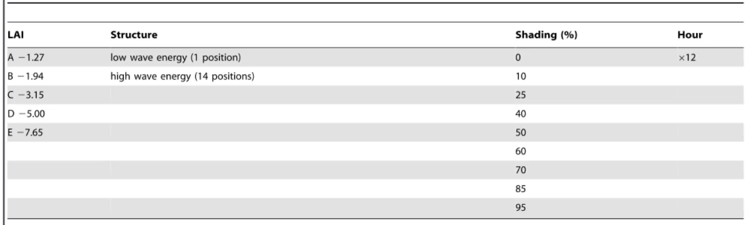
Table 1.Modelling experiment design.
LAI Structure Shading (%) Hour
A21.27 low wave energy (1 position) 0 612
B21.94 high wave energy (14 positions) 10
C23.15 25
D25.00 40
E27.65 50
60
70
85
95
A fully-factored set of model runs were performed for each of five LAI treatments, 15 canopy structures and nine shading treatments over 12 hourly diurnal intervals, a total of 8100 runs.
Results
Optical model validation
The sky radiance and water column model produced a daily top of canopy PAR dose of 11.0 mol quanta m22, whereas the comparablein-situmeasured average daily PAR irradiance over 3 months was 19.0 mol quanta m22 [9]. Since our study was primarily concerned with the relative effect of the shading treatments and LAI this discrepancy is not of great importance, but could be due to: 1) the accuracy of the libRadtran sky radiance model (no validation data available); 2) the accuracy of the Odyssey PAR sensors, which can have issues in long-term stability (Slivkoff, pers. comm.), or; 3) the model water columnkd(PAR),
which was at the upper range compared to measurements taken during the empirical study (0.2 vs. 0.070.19). This deviation in
kd(PAR) does provide an almost exact explanation for the
discrepancy, but sincekd(PAR) is a wavelength-integrated output
of the model parameterised on spectral IOPs for absorption and backscatter it is not trivial to set an arbitrary value ofkd(PAR). In
the scope of this study, using the closest IOP set from actual measured data [34] was considered adequate. In reality the daily measured PAR was sometimes above and sometimes below the model value, so all things considered the modelled canopy PAR dose was reasonable and the discrepancy is inconsequential to the subsequent interpretation of the results.
The percentage of the incident top of canopy PAR irradiance transmitted to the substrate, as a function of leaf area index, validated well against empirical data (Fig. 3). The empirical data showed wide variation, but the modelled transmitted irradiances corresponded very closely to the upper bound of the empirical data. This is to be expected, since some of the real canopies contained free standing and epiphytic macroalgae which would have reduced the transmission beyond that described by theA. griffithiiLAI alone. The upper bound points most likely represent the most monospecificA. griffithiicanopies and correspond best to the model. An exponential function fit to the model data (n= 28) gaver2
of 0.96, the fit of all 27 empirical data points to that same function gives an r2
of 0.73. However, if only four outliers are removed (Fig. 3) the empirical datar2rises to 0.90. The model and empirical data therefore compare well, especially given the practical difficulty in making accurate within-canopy light measurements.
The performance of the model in terms of energy conservation was demonstrated in the subset of runs for which water absorption was set to zero. For the majority of runs energy losses were less than 2% and for all runs they were less than 3%. In practice, when water absorption is non-zero, energy conservation performance would be better than these figures suggest. The current model implementation requires water absorption to be set to zero for energy accounting, but this in itself removes a damping effect on the multiple scattering and increases energy losses through numerical errors. Therefore the model solutions for leaf incident irradiance can be considered, at worst, slight underestimates by around 2%.
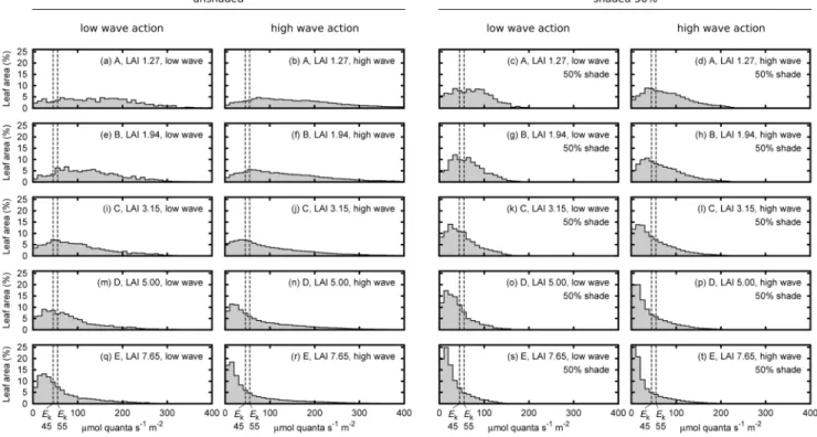
Effect of canopy structure and position on leaf level PAR As expected, the distribution of leaf level PAR irradiance became increasingly skewed to lower values as LAI increased (Figs. 4a, e, i, m, q). In low LAI canopies the distribution of PAR over leaf area was almost flat: leaf tissue received a wide range of PAR with almost equal probability, and much of it was above saturating irradiance at mid-day under the model conditions of clear sky and moderately clear water. In denser canopies the leaf level light distribution had a long high-end tail: many leaves
received light belowEk, but a few leaves received very high light
(Fig. 4i). Overall the pattern was clearly linked to the relative openness or self-shading within the canopies. The range ofEkof
45 to 55mmol quanta m22s21was generally small compared to range of irradiances the leaves experienced, but this was more true for the lower LAI and unshaded treatments (Fig. 4).
The treatments of canopy position of upright or moving under wave action appeared to have little effect on leaf level PAR irradiance (e.g. Fig. 4a vs. 4b). Numerically the canopy movement slightly reduced the daily integrated percentage of saturated leaf area for all but the lowest LAI (Fig. 5). However overall there was not a statistically significant difference at either Ek of 45 or
55mmol quanta m22s21(paired valuet-test,p.0.05). Therefore there is no evidence from our data that canopy movement affects time-integrated light capture. However the instantaneous light capture has a high variation under movement. While the standard deviation was 10–20% of the mean (Fig. 5) at some individual time points the saturated leaf area was up to 50% more or less than the mean. As expected, shading scaled thex-axis position of leaf-level irradiance distribution plots by the corresponding factor. That is, halving the top of canopy irradiance halved the leaf level incident irradiance at every leaf (Figs. 4b, d, f, h, etc.).
Diurnally accumulated saturated leaf area
The accumulated percentage of leaf area above saturation over a twelve-hour day showed a complex relationship between both shading and LAI (Fig. 6). While, as expected, increasing either shading or LAI monotonically decreased the accumulated percentage of leaf area above saturation, the shape of the function was non-linear and there was an interaction between shading and LAI (Fig. 6a). The contour lines in Figure 6a make clear the trade-Figure 3. Percentage of downwelling top of canopy PAR irradiance reaching the substrate, as a function of LAI.Results for empirical in-situ measurements (data 1 and 2) and modelled estimates (model) are shown. Curve fit to model data points isy= 100 * exp(20.296LAI).6(data 2) - are 26 individual coincident measurements
of LAI and irradiance above and below the canopy.^(data 1) is a single point based on a site mean of 13 LAI determinations from 2.84 to 4.09 and a set of associated but not spatially co-incident light measurements, error bars are one S.D. The four encircled points are the outliers referred to in the text. Transmittance data collection is described in McMahon and Lavery 2014 and corresponding LAI is unpublished data from Lavery et al. 2009.
N
are 25 model runs including both those described in detail and some additional runs. In the models runs solar zenith angle was approximately 28u.off between leaf area index and light with respect to the saturation state of the canopy. These lines show equal points in the LAI– shading function space, so for example a canopy of LAI 5.5 with no shading was equivalent to LAI 2.0 with 50% shading, with respect to the diurnally accumulated saturation of relative leaf area. The potential acclimation range ofEkfrom 45 to 55mmol
quanta m22s21 (assuming water temperature at approx. 23uC) added a degree of freedom to the LAI-shading relationship approximately equivalent to 1 unit of LAI at low shading (e.g. along thex-axis of Fig. 6a), but this increased as shading increased to 60% or more (Fig. 6a). Therefore at low shading modifyingEk
over the suggested range is equivalent to changing LAI by plus or minus one half.
For the high wave action treatment there is a small qualitative difference in the position of the contour lines in low LAI and low shading region as compared to the upright low wave action treatment (Fig. 6b vs. 6a). However a sensitivity analysis of the data tables underlying Figures 6a and 6b showed that these differences are equivalent to an error in the shading percentage of only 6 points or less. In other words, if in a practical application shading were quantified at discrete levels of 0, 5, 10, 15% etc. then the difference between upright and moving canopies would be negligible.
Discussion
Geometric optical modelling of seagrass canopies and validation
In terms of the geometrical optical modelling of seagrass canopies, the results presented here corroborate those of Hedley and Enrı´quez [25], showing that it is possible to construct a physical three dimensional model of a seagrass canopy and obtain acceptable validation against in-situ light measurements. Through-canopy transmission was estimated accurately for pure
Amphiboliscanopies, but the importance of considering epiphytes or other canopy constituents was underlined by the high variability of the empirical data, which in some cases had lower light penetration than the model predicted based onAmphibolisLAI alone.
With respect to morphological complexity,A. griffithiiis on the more complex end of the spectrum in comparison to strap leaf morphologies ofThalassiaand many other seagrass species [36], to which this modelling framework was previously confined. Figure 4. Distribution of leaf saturation state in the canopy in terms of percentage of leaf area at midday.Treatments are upright low wave action canopy positions and the average over the high wave action movement positions (left columns), and the same for 50% shading (right columns), for the five LAI treatments. The estimated photosynthetic saturation irradiances,Ek, of 45 and 55mmol quanta m22s21inferred from Masini and Manning (1997) are shown as vertical dotted lines.
doi:10.1371/journal.pone.0111454.g004
Therefore the potential for future models of other seagrass species is good as these two examples capture the range in canopy complexity. Hedley and Enrı´quez [25] used profiles of light through the canopy to derive a diffuse attenuation profile,kd, for
validation. In this study only light measurements at the top and bottom of the canopy were available. However, this simpler validation may be preferable and adequate. In practice, empirical measurements of light profiles within canopies are difficult to make, and rarely fit well to exponential attenuation with depth. The measurements at the top and bottom of the canopy are the strongest ‘‘signal’’ for within-canopy attenuation and can be used to derivekdif canopy height is known. So in future empirical work
to which such modelling may be subsequently applied, we recommend measuring downwelling irradiance at the top and bottom of canopies, together with canopy height and LAI.
Influence of shading, LAI and position on diurnal leaf photosynthetic saturation
The previous empirical shading study on A. griffithii [9] quantified the change in Hsat induced by shading, i.e. the total
number of hours of top-of-canopy irradiance that was above photosynthetic saturation, as compared to the unshaded treat-ments. This quantity, summed over time, was demonstrated as a good indicator of changes in canopy biomass and capacity for subsequent recovery. However Hsat relates the top of canopy
irradiance to leaf-level photosynthetic saturation irradiance and so ignores canopy self-shading and other structural factors, which therefore introduce an additional degree of freedom. Here, we factor in the canopy structure by considering the percentage of the canopy leaf area above saturating irradiance accumulated over time, HA
sat, with units of % leaf area6hour. This descriptor extendsHsatby reducing to a single number the interaction of the
duration of saturating irradiance and the canopy self-shading. It can be roughly interpreted as the daily ratio of saturated photosynthesis to leaf area at canopy scale, and ranges from 0 to 1200 for plants completely saturated for 12 hours of daylight.
Considering the variation in HAsat with leaf area index and
shading, as expected LAI has a strong effect on diurnal leaf saturation state (Fig. 6.). A change in LAI from 1 to 7 has as much effect as 60% shading (Fig. 6a), so the ambient light field cannot be treated independently from the canopy structure when photosyn-thetic processes at leaf level are of interest. Furthermore, the relationship between LAI and both shading and leaf saturation
state is a non-linear interaction; Figure 6 represents a curved surface in both axes of shading and LAI. This occurs because while leaf level irradiance is a linear function of canopy level irradiance, the leaf level photosynthetic response is not a linear function of irradiance when the irradiance approaches or exceeds
Ek. As leaf level irradiance approaches and exceeds Ek the
photosynthetic response levels off at Pmax. In general, since
photosynthesis versus irradiance curves are non-linear in the region of the saturating irradiance any derived measure of leaf level photosynthetic activity will have a complex relationship with LAI unless all leaves are well below saturating irradiance.
Within this study there is no statistically significant evidence to support the statement that canopy movement effects light capture and photosynthetic response. Qualitatively it is interesting that under movement the lowest LAI canopy experienced an increase in daily saturation whereas the higher LAI canopies were systematically lower (Fig. 5). To test the statistical significance of this observation would require substantial further modelling effort and was outside the scope of this study, however at low LAIs sideways movement may serve to enhance light collection by spreading leaves out horizontally and making them insensitive to the directionality of incident light. Under wave action such flattening is intermittent and as we have shown here is not a factor of great photosynthetic significance. Additionally, under these conditions the optical consequences of surface waves and sediment resuspension should also be considered and may be more significant [37]. However, in other systems and species, canopy flattening can be a result of shallow water depth or tidal or estuarine flow [38]. In this case the semi-constant flattening of the canopy may be of optical significance.
Potential for LAI modification as an acclimation response Figure 6 indicates that modification of LAI is a possible response to maintain the saturation state of the canopy under reduced or enhanced light conditions. This role of morphological plasticity has been demonstrated in a number of experimental studies (e.g. [39]) and hypothesized as a regulatory mechanism in
Thalassia[13]. From our model data (Fig. 6), if a canopy of LAI 7 is observed to reduce to LAI 4 after a period of 40% reduction in light, this loss of biomass might be interpreted as a trajectory of canopy decline but alternative interpretation is that of an acclimation response to maintain the leaf level photosynthetic state. This interpretation is independent of the mechanism by which it occurs. Leaf mortality might be considered just a by-Figure 6. Time accumulated percentage of leaf area irradiated above photosynthetic saturation irradiance.The colour scale shows
HAsat, the ‘‘percentage leaf area hours’’ aboveEk, as a function of LAI and shading. (a) is for upright low wave action canopy structures, (b) is for the average over the high wave energy canopy positions. Contour lines are isoclines based on the mid value ofEkequal to 50mmol quanta m22s21 while the surrounding greyed region shows the limits forEkof 45 to 55mmol quanta m22s21. The isoclines are located atHAsatof 50, 100, 200, and then steps of 100 up to 800% leaf area hours.
product of inadequate light to maintain respiration, but if the net effect is a return to an unstressed leaf-level light regime then the distinction between a compensatory morphological adjustment and a decline is at best ambiguous. This argument is of course dependent on the definition of ‘decline’; it does not apply if net productivity per unit area rather than biomass is the criteria. Here, by ‘decline’ we mean an implied trajectory toward canopy eradication.
Under the interpretation of potential acclimation a key question is whether the reduction in LAI remains on the isocline for canopy saturation state (i.e. the contour lines in Fig. 6). A canopy that moves on a trajectory through LAI–shading ‘space’ such that it stays on a contour line is experiencing the same time integrated percentage of its leaf area at saturating irradiance (see A to E in Fig. 7). That is, it experiences the same daily photosynthetic saturation in relation to its leaf biomass. We might therefore hypothesise that if a canopy can sustainably exist at one point on anHAsatisocline, canopies can also sustainably exist at other points
on that line, all other things being equal. Movement along an isocline can occur purely by modification of the LAI, alternative acclimation responses such as modification ofEkat the leaf-level
will enable movement perpendicular to the isoclines, illustrated by the range around the isoclines in Figures 6 and 7 delimited byEk
of 45 to 55mmol quanta m22s21. Ignoring the latter possibility, and focussing on LAI modification alone, the prospects for long term survival of a canopy under a change in light environment can be estimated by following the isocline from its current location in LAI-shading space to the new light environment (y-axis) location. If at this location the LAI is greater than zero (judged by extrapolation), then the canopy could survive by thinning out to this LAI, at which point it will have the same relative photosynthetic saturation of its leaf area. In the following section we use this concept to interpret the results from the previous empirical shading experiment [9].
Canopy trajectories in LAI and shading space
In the post-summer treatment of the shading experiment of Lavery et al. [9] canopies with an LAI of,4 had reduced to an
LAI of,2 after three months of 84% shading. This change in LAI
and shading can be represented as a trajectory on theHAsatmap:
Figure 7, point A to B. At 6 months of shading the LAI had reduced to one and by 9 months the canopy was almost eradicated
and did not subsequently recover (Fig. 7, point C). Assuming for the moment thatHA
sat, the accumulated percentage area of leaf
saturation aboveEk, is a measure relevant to canopy sustainability
then Figure 7 indicates that such a measure could have predictive power for canopy survival. In the previous section we postulated that canopies can move along the isoclines by modification of LAI alone. The initial reduction of LAI in the empirical data (Fig. 7, point A to B) occurred in the first three months in response to 84% shading. The trajectory cuts across the isoclines because there is a time lag as the canopy cannot become thinner instantaneously. At three months (Fig. 7, point B) the LAI has reduced to 2 but the shading is extreme so at the leaf level the light environment is still very much reduced. There can be two response pathways, either physiological changes may allow the canopy to exist on the new isocline, such as the mobilisation of stored reserves [40] or reductions in the saturating irradiance [23], or if such processes cannot bring about sufficient change then further LAI reduction is required in an attempt to return to an isocline closer to the original. In this case following the isocline to the right and extrapolating to the intercept with thex-axis it is clear that the light environment is equivalent to a canopy with huge LAI of at least 20+ in the original un-shaded situation. For the canopy to survive would require physiological changes that would permit canopies of these high LAIs to exist normally in this environment. Such canopies did not exist, hence physiological changes are insufficient (it is clear from Fig. 7 that variation in Ek is
inadequate), hence the LAI continued to decrease and eventually the canopy was eradicated (Fig. 6, Point C).
The previous example is a straightforward case of severe light limitation, but with moderate shading (for example 40%, Fig. 7) the situation is more complicated. The empirical data of Lavery et al. [9] only contained shading at a minimum of 81% so the example of 40% in Figure 7 is hypothetical. If a situation of 40% shading is introduced, assuming the validity ofHA
sat, it is clear that
the canopy could survive by reducing LAI from 4 to 1 (moving along the isocline from point A to point E, Fig. 7). However, because of the time lag in reducing LAI, an initial trajectory in which LAI partially reduces (A to D, Fig. 7) is realistic and is likely to include physiological responses in tandem. For example Ek
could decrease, but at LAI around 3 the range ofEkfrom 45 to 55
only allows accommodation of up to 20% shading at the most (Fig. 7). The existence of a time lag is supported by studies on different seagrass species that have incorporated less extreme shading treatments over short time-scales; physiological changes such as increases in chlorophyll and reduction in LAI occur after longer durations of reduced light [39]. At point D in Figure 7 the canopy lies on an isocline that represents a canopy of LAI 5.5 in the unshaded environment. If such canopies can sustainably exist, at the same depth, water clarity etc. then the canopy may survive at LAI of 2 to 3 (point D), rather than reducing LAI to 1 (point E). Either way, Figure 7 has predictive power for the canopy response in that if it is anticipated a 40% shading event may occur, e.g., from dredging activities, then it is clear that a canopy that is sustainable at LAI of 4 could reduce to LAI of 1, or, could induce physiological changes to maintain an LAI higher than 1, but in the latter case only if canopies greater than LAI of 4 currently exist in that environment.
The possible trajectories in LAI-shading space of Figure 7 are dependent on the capability and time constants of other physiological acclimation mechanisms. These mechanisms could include adjustments to photosystem kinetics to increase the efficiency (i.e. lowerEk), increases in chlorophyll content and a:b
ratio to enhance light capture, or mobilisation of stored carbohydrates for maintenance and growth of the existing leaf Figure 7. Trajectories of canopies from empirical shading
experiment and hypothetical example. Underlying plot is as described in the caption of Figure 6a.
biomass [7]. To our knowledge there is no published data on photo-acclimation inA. griffithiiunder changing light conditions. However, unpublished data by co-author McMahon shows that under high levels of shading there are reductions in the saturating irradiance and other photo-acclimation responses, which maintain electron transport rates at unshaded values, but there is a time-limit over which this photo-acclimation is maintained of around 21 days. Therefore, the model as we have developed here is very relevant for predicting impacts associated with longer term reductions in light of over three weeks or more.
Other measures of canopy scale photosynthetic response to light
In the previous discussion we have assumed that the concept of isoclines of equal light environment’ with respect toHAsatis valid.
Alternative measures may be more appropriate but this does not affect the primary concept that canopy self-shading can be equivalent to environmental shading, and that there are two mechanisms of photosynthetic acclimation: physiological and via canopy structure. Any alternative measure of the photosyntheti-cally relevant light environment would likely have a similar form to that of Figures 6 and 7. The interaction of self-shading and the non-linearity of leaf-level photosynthesis must inevitably result in a complex canopy scale response to LAI and the light environment for all canopies that are subjected to irradiances above photosyn-thetic saturation. Another candidate measure would be the integration of photosynthesis over time, i.e. to propagate the leaf-level light through a photosynthesis versus irradiance (P-I) curve to give an integrated photosynthesis measure equivalent to
mmol O2evolution. In addition, plots of actual top of canopy PAR
light levels may have greater descriptive power than percentage shading (Figures 6 and 7). Lavery et al. [9] observed different canopy changes at similar shading levels and interpreted these as being due to differences in the absolute light levels. In this study we suggested HA
sat as a simple extension of the top-of canopyHsat,
since that measure has been demonstrated to have predictive power for canopy sustainability [8,9] and has been used in management contexts, and percentage shading was employed as a mirror of the empirical treatments. Clearly, there are many opportunities for further experiments and modelling to determine the most relevant measure of canopy photosynthetic response, the key point being that that measure needs to include within-canopy light propagation.
Conclusions
Three dimensional canopy modelling of Amphibolis griffithii
has revealed that the interaction of light levels and canopy density on canopy-scale photosynthetic activity is complex and non-linear, in particular due to the non-linearity of leaf-level photosynthesis at saturating irradiance. The accumulated percentage area of leaf saturation above saturating irradiance,HA
sat, was proposed as a
measure relevant to canopy sustainability, based on extension of the equivalent top-of-canopy measure Hsat that has previously
proved useful. The available empirical data were not sufficient to evaluate the efficacy of HAsat due to lack of lower shading
treatments. Evaluating this measure and other candidates such as integrated leaf-level photosynthesis requires further experimental work. Nevertheless the principle has been demonstrated that plots of equal light environment’ (Fig. 6) produced for different seagrass species, water depths, and water column optical properties could have practical management applications for predicting and interpreting canopy changes under light reduction events. Reduction in seagrass density in response to shading must be interpreted in terms of the leaf-level light environment. While physiological responses are also important, existing canopies in the same environment can provide information of the limits of physiological acclimation, and indicate if change in light levels will induce a trajectory to steady state sustainability, or to eradication. An important future step is to understand the time constants in change and recovery trajectories, to determine how long shading events can be tolerated and the required recovery periods. This information will be invaluable to coastal management.
Acknowledgments
J Hedley wishes to acknowledge Susana Enrı´quez, whose ideas and insight have informed the work described here. K McMahon acknowledges the collaboration with P S Lavery, which provided background for this research, L Twomey and M Westera from BMT Oceanica Pty Ltd for insights contributing to this work and N Dunham for canopy measure-ments.
Author Contributions
Conceived and designed the experiments: JH KM PF. Performed the experiments: JH KM. Analyzed the data: JH KM PF. Contributed reagents/materials/analysis tools: JH KM. Contributed to the writing of the manuscript: JH KM PF.
References
1. Orth RJ, Carruthers TJB, Dennison WC, Duarte CM, Forqurean JW, et al. (2006) A global crisis for seagrass ecosystems. Bioscience 56: 987–996. 2. Costanza R, d’Arge R, de Groot R, Farber S, Grasso M, et al. (1997) The value
of the world’s ecosystem services and natural capital. Nature 387: 253–260. 3. Fourqurean JW, Duarte CM, Kennedy N, Marba` N, Holmer M, et al. (2012)
Seagrass ecosystems as a globally significant carbon stock. Nature Geoscience 5: 505–509.
4. Waycott M, Duarte CM, Carruthers TJB, Orth RJ, Dennison WC, et al. (2009) Accelerating loss of seagrasses across the globe threatens coastal ecosystems. Proceedings of the National Academy of Sciences 106: 12377–12381. 5. Grech A, Chartrand-Miller K, Erftemeijer P, Fonseca M, McKenzie L, et al.
(2012) A comparison of threats, vulnerabilities and management approaches in global seagrass bioregions. Environmental Research Letters 7: 024006. 6. Grech A, Coles R, Marsh H (2011) A broad-scale assessment of the risk to
coastal seagrasses from cumulative threats. Marine Policy 35: 560–567. 7. McMahon K, Collier C, Lavery PS (2013) Identifying robust bioindicators of
light stress in seagrasses: A meta-analysis. Ecological Indicators 30: 7–15. 8. Collier CJ, Waycott M, McKenzie LJ (2012) Light thresholds derived from
seagrass loss in the coastal zone of the northern Great Barrier Reef, Australia. Ecological Indicators 23: 211–219.
9. Lavery PS, McMahon K, Mulligan M, Tennyson A (2009) Interactive effects of timing, intensity and duration of experimental shading onAmphibolis griffithii. Marine Ecology Progress Series 394: 21–33.
10. Lambers H, Chapin FS, Pons TL (1998) Plant physiological ecology. New York: Springer. 540 pp.
11. Kirk JTO (1994). Light and photosynthesis in aquatic ecosystems. Cambridge: Cambridge Press. 528 pp.
12. Ralph PJ, Durako MJ, Enrı´quez S, Collier CJ, Doblin MA (2007) Impact of light limitation on seagrasses. Journal of Experimental Marine Biology and Ecology 350: 176–193.
13. Cayabyab NM, Enrı´quez S (2007) Leaf photoacclimatory responses of the tropical seagrassThalassia testudinumunder mesocosm conditions: a mecha-nistic scaling-up study. New Phytol 176: 108–123.
14. Masini RJ, Manning CR (1997) The photosynthetic responses to irradiance and temperature of four meadow-forming seagrasses. Aquatic Botany 58: 21–36. 15. Duarte CM, Marba N, Krause-Jensen D, Sanchez-Camacho M (2007) Testing
the predictive power of seagrass depth limit models. Estuaries and Coasts 30: 652–656.
16. O’Brien KR, Grinham A, Roelfsema CM, Saunders MI, Dennison WC (2011) Viability criteria for the presence of the seagrassZostera muelleriin Moreton Bay, based on benthic light dose. In: MODSIM 2011: International Congress on Modelling and Simulation, Proceedings. Modelling and Simulation Society of Australia and New Zealand (MODSIM 2011), Perth, Australia, 12–16 December 2011. 4127–4133.
18. Dennison WC, Orth RJ, Moore KA, Court Stevenson J, Carter V, et al. (1993) Assessing water quality with submersed aquatic vegetation: habitat requirements as barometers of Chesapeake Bay health. BioScience 43: 86–94.
19. Gacia E, Marba N, Cebrian J, Vaquer-Sunyer R, Garcias-Bonet N, et al. (2012) Thresholds of irradiance for seagrassPosidonia oceanicameadow metabolism. Mar Ecol Prog Ser 466: 69–79.
20. Dennison WC, Alberte RS (1985) Role of daily light period in the depth distribution ofZostera marina(eelgrass). Mar Ecol Prog Ser 25: 51–61. 21. Enrı´quez S, Merino M, Iglesias-Prieto R (2002) Variations in the photosynthetic
performance along the leaves of the tropical seagrassThalassia testudinum. Marine Biology 140: 891–900.
22. Fourqurean JW, Zieman JC (1991) Photosynthesis, respiration and whole plant carbon budget of the seagrassThalassia testudinum. Mar Ecol Prog Ser 69: 161– 170.
23. Collier CJ, Lavery PS, Masini RJ, Ralph PJ (2007) Morphological, growth and meadow characteristics of the seagrassPosidonia sinuosaalong a depth-related gradient of light availability. Mar Ecol Prog Ser 337: 103–115.
24. Carruthers TJB, Walker DI (1997) Light climate and energy flow in the seagrass canopy ofAmphibolis griffithii(J.M.Black) den Hartog. Oecologia 109: 335–341. 25. Hedley JD, Enrı´quez S (2010) Optical properties of canopies of the tropical seagrass Thalassia testudinum estimated by a three-dimensional radiative transfer model. Limnology and Oceanography 55: 1537–1550.
26. Zimmerman R (2006) Light and photosynthesis in seagrass meadows. In: Larkum AWD, Orth RJ, Duarte C, editors. Seagrasses: Biology, ecology and conservation. Springer. 303–321.
27. Hedley JD (2008) A three-dimensional radiative transfer model for shallow water environments. Optics Express 16: 21887–21902.
28. McMahon K, Lavery PS (2014) Canopy-scale modifications of the seagrass Amphibolis griffithiiin response to and recovery from light reduction. Journal of Experimental Marine Biology and Ecology 455: 38–44.
29. House DH, Breen DE (2000) Cloth modeling and animation. Massachusetts: A. K. Peters. 344 p.
30. Mayer B, Kylling A (2005) The libRadtran software package for radiative transfer calculations – description and examples of use. Atmospheric Chemistry and Physics 5: 1855–1877.
31. Grant RH, Heisler GM, Gao W (1996) Photosynthetically-active radiation: Sky radiance distributions under clear and overcast conditions. Agricultural and Forest Meteorology 82: 267–292.
32. Mobley CD (1994) Light and Water. San Diego: Academic Press. 608 p. 33. Mobley CD, Sundman L (2000) HydroLight 4.1 user’s guide. Sequoia Scientific.
Available: http://www.sequoiasci.com/products/Hydrolight.aspx.
34. Hedley JD, Roelfsema CM, Phinn SR, Mumby PJ (2012). Environmental and sensor limitations in optical remote sensing of coral reefs: Implications for monitoring and sensor design. Remote Sensing 4: 271–302.
35. Durako MJ (2007) Leaf optical properties and photosynthetic leaf absorptances in several Australian seagrasses. Aquatic Botany 87: 83–89.
36. Green EP, Short F (2004) World atlas of seagrasses. Berkeley: University of California Press. 320 p.
37. Pedersen TM, Gallegos CL, Nielsen SL (2012) Influence of near-bottom re-suspended sediment on benthic light availability. Estuarine, Coastal and Shelf Science 106: 93–101.
38. Koch E, Gust G (1999) Water flow in tide and wave dominated beds of the seagrassThalassia testudinum. Mar Ecol Prog Ser 184: 63–72.
39. Collier CJ, Waycott M, Ospina AG (2012b) Responses of four Indo-West Pacific seagrass species to shading. Marine Pollution Bulletin 65: 342–354.