Transactions of the VŠB – Technical University of Ostrava, Mechanical Series No. 3, 2010, vol. LVI
article No. 1818
Martin KOSÍK*, Jiří FÜRST**
DESCRIPTION AND APPLICATION OF THE CE-SE SCHEME
POPIS A APLIKACE CE-SE SCHÉMATU
Abstract
The CE-SE scheme is new numerical methodology for conservation laws. It was developed by Dr.Chang of NASA Glenn Research Center and his collaborators. The 1D and 2D variant of CE-SE scheme for scalar convection and for Euler equations for incompressible flows is described. The CE-SE scheme is compared with classical schemes in 1D. The solution to inviscid incompressible flow in GAMM channel in 2D is presented.
Abstrakt
CE-SE schéma je nová numerická metoda pro řešení zákonů zachování. V článku je popsána 1D a 2D varianta CE-SE schématu pro skalární rovnici a pro Eulerovy rovnice popisující nestlačitelné proudění. CE-SE schéma je srovnáváno s klasickými schématy v 1D a ve 2D je prezentováno řešení nevazkého, nestlačitelného proudění v GAMM kanále.
1 INTRODUCTION
The CE-SE (Conservation Element – Solution Element) scheme is new numerical methodology for conservation laws. It was developed by Dr. Chang of NASA Glenn Research Center and collaborators. The concept and methodology of this method are significantly different from those in the well-established traditional numerical methods. The flux is conserved in space and time. They are treated equally. The dependent variables and their derivatives are considered as individual unknowns to be solved simultaneously at each grid point [1-2].
2 1D AND 2D VERSIONS OF CE-SE SCHEME BE DESCRIBE
2.1 One-dimensional version be described
Consider the linear 1D unsteady advection equation
0
,
,
0
a
R
a
x
u
a
t
u
(1)
where constant a is the advection speed and u is an arbitrary scalar function. In the space-time Euclidean space
E
2, the integral form of (1) is
0
.
d
n
h
(2)
*
Ing., CTU in Prague, Faculty of Mechanical Engineering, Department of Technical Mathematics, Karlovo nám. 13, Prague, tel. (+420) 22 435 7539, e-mail [email protected]
**
where
h
au
,
u
and is the boundary of arbitrary space-time region of in, is normal vector of boundry
2
E
d
n
dt
,
dx
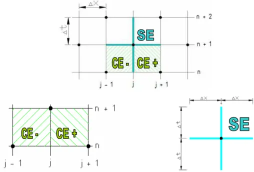
. The conservation element (CE) andsolution element (SE) are the two basic elements. They are depicted in Fig. 1.
Fig. 1 Position of CE and SE elements in 1D
At each SE element [j, n+1], u(x,t) is approximated by the first-order Taylor series expansion:
1
1
1
1
*1
,
;
,
t
j
n
u
jn
u
x njx
x
j
u
t njt
t
nx
u
(3)where,
u
nj1 ,(
u
x)
nj1 and(
u
t)
nj1 are constant. After inserting ofu
*toh
, we geth
au
*,
u
*
. The assumption thatu
satisfies (1) implies . We integrate equation (2)around and we get two CE elements:
*
u
1)
nj1
(
)
(
u
t nj
a
u
xCE
1
1
2
1
0
2
1
1
,
4
1 1 1
2 1
2
2
nj
n j n
j x n
j
x
u
u
x
u
u
n
j
F
x
(4)where
(
a
.
t
)
/
x
. From equation (4) we obtain two unknownsu
nj and(
u
x)
nj :
n
j x n
j x n
j n
j n
j
u
u
x
u
u
u
1 1 1 2 1 14
1
1
1
2
1
(5)
n
j x n
j x n
j n j n
j
x
u
u
u
u
x
u
1 2 21
4
1 11
21
11
11
2
1
(6)2.2 Two-dimensional version be described
Two-dimensional version is described at cartesian mesh. We study inviscid incompressible flow described by the set of Euler equations with artificial compressibility method. Those equations in matrix and quasi-linear form, can be written as:
0
x yt
W
W
G
W
W
F
W
(7)
p
p
p
v
uv
v
G
uv
p
u
u
F
v
u
p
W
~
,
,
,
,
2
~
,
,
,
,
2
~
,
~
where
W
F
is jacobian’s of flux F,
W
G
is jacobian’s of flux G, p is pressure,
is density(constant) and u, v are velocities. From Eq.(7) we can get
W
tn :j i, y x t
W
W
G
W
W
F
W
(8)Fig.2 Position of CE and SE elements in 2D
Fig. 2 shows four CE elements, one from four is and the
SE element is shown with black points . For SE element we get
from Taylor series expansion in space-time:
1 1 1
1
n n n n n n n n
D
C
B
A
D
C
B
A
1 1 11
n n n n
F
C
E
n n n nA
F
C
E
A
n
n
t j i n y j i n x n j
i
W
x
x
W
y
y
W
t
t
W
t
y
x
W
SE
t
y
x
j i j i ji
, , , , , ,,
,
,
,
(9)
n n nnBC D n n n n n n n n n n n n
A B C B C
BC B A B A AB D C B A n n
G
F
n
G
F
n
W
dxdy
W
1 1 1 1 1 1 1 1)
,
(
)
,
(
1
(10)
(
,
)
(
,
)
0
1 1 1 1
n n n n n n nn DA D A
DA D
C D C
CD
F
G
n
F
G
n
where , , and are normal vectors at appropriate for sides. We apply this equation at four CE elements around SE element. We get four values of W in time-step n+1, and then we get W in mesh point i, j and time-step n+1:
AB
n
n
BC
CD
n
n
DA4
3
2
1
4
.
4
3
.
3
2
.
2
1
.
1
1 ,CE
CE
CE
CE
W
CE
W
CE
W
CE
W
CE
W
inj
(11)Values of derivatives
W
xn1 andW
yn1 in a SE element are calculated with least squares method.3 COMPUTATIONAL RESULTS
3.1 One-dimensional scalar problem
We will solve initial-boundary value problem for scalar equation:
0
x tau
u
(12)with initial condition (13), where a=1,
x
0
;
1
, and boundary condition isu
0
,
t
t
0
. We compare exact solution with two numericals schemes: first order upwind scheme and new CE-SE scheme for initial condition:
u
x
,
0
0
x
0
,
0
.
25
0
.
5
,
1
(13)
x
,
0
1
cos
8
x
/
2
x
0
.
25
,
0
.
5
u
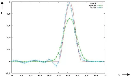
Fig. 3 shows solution in time t = 0.25 and space step
x
= 0.02. Solution with upwind scheme doesn’t produce any spurious oscillations, but is very inaccurate. Solution with CE-SE scheme is more accurate, but produces some oscillations in places with discontinuity in high derivatives.u
x
3.2 Two-dimensional problem
We demonstrate of CE-SE method in two-dimensional problem on flow in GAMM channel. Geometry of GAMM channel is shown in Fig. 4, where
uw and
lw are up-wall and down-wall, is inlet of flow to channel and is outlet of channel.i
o
uw
o
i
lw
Fig. 4 Geometry of GAAM channel
We look for solution of inviscid, incompressible flows with artificial compressibility. This flow described of Euler equations (7). Constant pressure
p
~
= 1 and velocity u = 1, v = 0 was taken asthe initial condition. Boundary conditions at the inlet are u = 1 and v = 0,
~
p
is extrapolated, at theoutlet is
~
p
1
. It is realized by the so-called reflexion. For numerical solution in 2D we created and u and v are extrapolated. At the walls we use inpermeability condition algebraically generated mesh with 75x25 cells.
u
.
n
0
Fig. 5 shows the distribution of pressure in GAMM channel in form of isolines. Computed distribution of pressure is not completely symmetric, but the difference from theoretically correct symmetric solution is small.
Fig. 5 Isolines of pressure in GAMM channel
4 CONCLUSIONS
ACKNOWLEDGEMENTS
This work was supported by the Grant Agency of the Czech Technical University in Prague, grant No. SGS 10/244/OHK2/3T/12
REFERENCES
[1] CHANG S-C., New Numerical Framework for Solving Conservation Laws – The method of Space-Time Conservation Element and Solution Element , NASA , 1991, TM-104495
[2] CHANG S-C., Application of the Space-Time Conservation Element and Solution Element Method to One-Dimensional Advection-Diffusion Problems, NASA, 1999, TM-1999-209068 [3] R. DVORAK, K. KOZEL, Matematické modelování v aerodynamice, ČVUT, 1996,