Inferring Pairwise Interactions from Biological Data Using Maximum-Entropy Probability Models.

REVIEW

Inferring Pairwise Interactions from

Biological Data Using Maximum-Entropy

Probability Models

Richard R. Stein1*, Debora S. Marks2, Chris Sander1*

1Computational Biology Program, Sloan Kettering Institute, Memorial Sloan Kettering Cancer Center, New York, New York, United States of America,2Department of Systems Biology, Harvard Medical School, Boston, Massachusetts, United States of America

*maxent@sanderlab.org(RRS);maxent@sanderlab.org(CS)

Abstract

Maximum entropy-based inference methods have been successfully used to infer direct interactions from biological datasets such as gene expression data or sequence ensem-bles. Here, we review undirected pairwise maximum-entropy probability models in two cate-gories of data types, those with continuous and categorical random variables. As a concrete example, we present recently developed inference methods from the field of protein contact prediction and show that a basic set of assumptions leads to similar solution strategies for inferring the model parameters in both variable types. These parameters reflect interactive couplings between observables, which can be used to predict global properties of the bio-logical system. Such methods are applicable to the important problems of protein 3-D struc-ture prediction and association of gene–gene networks, and they enable potential

applications to the analysis of gene alteration patterns and to protein design.

Introduction

Modern high-throughput techniques allow for the quantitative analysis of various components of the cell. This ability opens the door to analyzing and understanding complex interaction pat-terns of cellular regulation, organization, and evolution. In the last few years,undirected pair-wise maximum-entropy probability modelshave been introduced to analyze biological data and have performed well, disentanglingdirect interactionsfrom artifacts introduced by inter-mediates or spurious coupling effects. Their performance has been studied for diverse prob-lems, such as gene network inference [1,2], analysis of neural populations [3,4], protein contact prediction [5–8], analysis of a text corpus [9], modeling of animal flocks [10], and prediction of multidrug effects [11]. Statistical inference methods using partial correlations in the context of graphical Gaussian models (GGMs) have led to similar results and provide a more intuitive understanding of direct versus indirect interactions by employing the concept of conditional independence [12,13].

Our goal here is to derive a unified framework for pairwise maximum-entropy probability models for continuous and categorical variables and to discuss some of the recent inference approaches presented in the field of protein contact prediction. The structure of the manuscript is as follows: (1) introduction and statement of the problem, (2) deriving the probabilistic OPEN ACCESS

Citation:Stein RR, Marks DS, Sander C (2015) Inferring Pairwise Interactions from Biological Data Using Maximum-Entropy Probability Models. PLoS Comput Biol 11(7): e1004182. doi:10.1371/journal. pcbi.1004182

Editor:Shi-Jie Chen, University of Missouri, UNITED STATES

Published:July 30, 2015

Copyright:© 2015 Stein et al. This is an open access article distributed under the terms of the Creative Commons Attribution License, which permits unrestricted use, distribution, and reproduction in any medium, provided the original author and source are credited.

Funding:This work was supported by NIH awards R01 GM106303 (DSM, CS, and RRS) and P41 GM103504 (CS). The funders had no role in the preparation of the manuscript.

model, (3) inference of interactions, (4) scoring functions for the pairwise interaction strengths, and (5) discussion of results, improvements and applications.

Better knowledge of these methods, along with links to existing implementations in terms of software packages, may be helpful to improve the quality of biological data analysis compared to standard correlation-based methods and increase our ability to make predictions of interac-tions that define the properties of a biological system. In the following, we highlight the power of inference methods based on the maximum-entropy assumption using two examples of bio-logical problems: inferring networks from gene expression data and residue contacts in pro-teins from multiple sequence alignments. We compare solutions obtained using (1)

correlation-based inference and (2) inference based on pairwise maximum-entropy probability models (or their incarnation in the continuous case, the multivariate Gaussian distribution).

Gene association networks

Pairwise associations between genes and proteins can be determined by a variety of data types, such as gene expression or protein abundance. Association between entities in these data types are commonly estimated by the samplePearson correlationcoefficient computed for each pair of variablesxiandxjfrom the set of random variablesx1,. . .,xL. In particular, forMgiven samples inLmeasured variables,x1

¼ ðx1 1;. . .;x

1 LÞ

T

;. . .;xM_{¼ ðx}M 1 ;. . .;x

M LÞ

T

2RL_{, it is} defined as,

rij:¼

^

Cij ffiffiffiffiffiffiffiffiffiffiffi

^

CiiC^jj

q ;

where_C^

ij:¼ 1 M

XM

m¼1ðx m i xiÞðx

m

j xjÞdenotes the (i,j)-element of the empirical covariance

matrixC^¼ ðC^ijÞi;j¼1;...;L. The sample mean operator provides the empirical mean from the

measured data and is defined asxi :¼ 1 M

XM

m¼1x m

i . A simple way to characterize dependencies

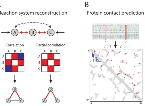
in data is to classify two variables as being dependent if the absolute value of their correlation coefficient is above a certain threshold (and independent otherwise) and then use those pairs to draw a so-called relevance network [14]. However, the Pearson correlation is a misleading mea-sure for direct dependence as it only reflects the association between two variables while ignor-ing the influence of the remaining ones. Therefore, the relevance network approach is not suitable to deduce direct interactions from a dataset [15–18]. Thepartial correlationbetween two variables removes the variational effect due to the influence of the remaining variables (Cramér [19], p. 306). To illustrate this, let’s take a simplified example with three random vari-ablesxA,xB,xC. Without loss of generality, we can scale each of these variables to zero-mean

and unit-standard deviation byxi7!ðxixiÞ ffiffiffiffiffiffi

^

Cii q

, which simplifies the correlation coeffi

-cient torijxixj. The sample partial correlation coefficient of a three-variable system between xAandxBgiven xCis then defined as [19,20]

rABC¼

rABrBCrAC

ffiffiffiffiffiffiffiffiffiffiffiffiffiffiffi

1r2

AC

p ffiffiffiffiffiffiffiffiffiffiffiffiffiffi

1r2

BC

p

ðC^1 ÞAB

ffiffiffiffiffiffiffiffiffiffiffiffiffiffiffiffiffiffiffiffiffiffiffiffiffiffiffiffiffiffi

ð_C^1_Þ

AAðC^1ÞBB

q :

The latter equivalence by Cramer’s rule holds if the empirical covariance matrix, ^

C ¼ ðC^ijÞi;j2fA;B;Cg, is invertible. Krumsiek et al. [21] studied the Pearson correlations and partial

Pearson’s correlations,rAB,rACrBC, versus the corresponding partial correlations,rABC,rACB,

rBCA, shows that variables A and C appear to be correlated when using Pearson’s correlation as

a dependency measure since both are highly correlated with variable B, which results in a false inferred reactionrAC. The strength of the incorrectly inferred interaction can be numerically large and therefore particularly misleading if there are multiple intermediate variables B [22]. The partial correlation analysis removes the effect of the mediating variable(s) B and correctly recovers the underlying interaction structure. This is always true for variables following a mul-tivariate Gaussian distribution, but also seems to work empirically on realistic systems as Krumsiek et al. [21] have shown for more complex reaction structures than the example pre-sented here.

Protein contact prediction

The idea that protein contacts can be extracted from the evolutionary family record was formu-lated and tested some time ago [23–26]. The principle used here is that slightly deleterious mutations are compensated during evolution by mutations of residues in contact in order to maintain the function and, by implication, the shape of the protein. Protein residues that are close in space in the folded protein are often mutated in a correlated manner. The main prob-lem here is that one has to disentangle the directly co-evolving residues and remove transitive correlations from the large number of other co-variations in protein sequences that arise due to statistical noise or phylogenetic sampling bias in the sequence family. Interactions not internal to the protein are, for example, evolutionary constraints on residues involved in

Fig 1. Reaction system reconstruction and protein contact prediction.Association results of correlation-based and maximum-entropy methods on biological data from anin silicoreaction system (A) and protein contacts (B). (A) Analysis by Pearson’s correlation yields interactions associating all three compounds A, B, and C, in contrast to the partial correlation approach which omits the“false”link between A and C. (Fig 1A based on [21].) (B) Protein contact prediction for the human RAS protein using the correlation-based mutual information, MI, and the maximum-entropy based direct information, DI, (blue and red, respectively). The 150 highest scoring contacts from both methods are plotted on the protein contacts from experimentally determined structure in gray. (Fig 1B based on [6].)

oligomerization, protein–protein, protein–substrate interactions [6,27,28]. In particular, the empirical single-site and pair frequency counts in residueiand in residuesiandjfor elements

s,oof the 20-element amino acid alphabet plus gap,fi(s) andfij(s,o), are extracted from a representative multiple sequence alignment under applied reweighting to account for biases due to undersampling. Correlated evolution in these positions was analyzed, e.g., by [29], by using themutual informationbetween residueiandj,

MIij¼ X

s;o

fijðs;oÞln

fijðs;oÞ fiðsÞfjðoÞ

!

:

Although results did show promise, an important improvement was made years later by using a maximum-entropy approach on the same setup [5–7,30]. In this framework, thedirect informationof residueiandjwas introduced by replacingfijin the mutual information byPdir

ij ,

DIij¼ X

s;o

Pdir

ij ðs;oÞln Pdir

ij ðs;oÞ fiðsÞfjðoÞ !

; ð1Þ

wherePdir

ij ðs;oÞ ¼ 1

Zijexpðeijðs;oÞ þ

~

hiðsÞ þh~jðoÞÞand~hiðsÞ;~hjðoÞandZijare chosen such

thatPdir

ij , which is based on a pairwise probability model of an amino acid sequence compatible

with the iso-structural sequence family, is consistent with the single-site frequency counts. In an approximative solution, [6,7] determined the contact strength between the amino acidssando

in positioniandj, respectively, by

eijðs;oÞ ’ ðC 1

ðs;o_ÞÞij: ð2Þ

Here, (C−1_(s,o))

ijdenotes the inverse element corresponding toCij(s,o)fij(s,o)−fi(s) fj(o) for amino acidss,ofrom a subset of 20 out of the 21 different states (the so-called gauge fixing, see below). The comparison of contact prediction results based on MI- and DI-score for the RAS human protein on top of the actual crystal structure shows a much more accurate pre-diction result when using the direct information instead of the mutual information (Fig 1B).

The next section lays the foundation to deriving maximum-entropy models for the two data types: continuous, as used in the first example, and categorical, as used in the second one. Sub-sequently, we will present inference techniques to solve for their interaction parameters.

Deriving the Probabilistic Model

Ideally, one would like to use a probabilistic model that is, on the one hand, able to capture all orders of directed interactions of all observables at play and, on the other hand, correctly repro-duces the observed and to-be-predicted frequencies. However, this would require a prohibi-tively large number of observed data points. For this reason, we restrict ourselves to

probabilistic models with terms up to second order, which we derive for continuous, real-val-ued variables, and extend this framework to models with categorical variables that are suitable, for example, to treat sequence information in the next section.

Model formulation for continuous random variables

continuously distributed on real values. In a biological example, these data originate from gene expression studies and each variablexicorresponds to the normalized mRNA level of a gene measured inMsamples. As an example, a recent pan-cancer study of The Cancer Genome Atlas (TCGA) provided mRNA levels fromM= 3,299 patient tumor samples from 12 cancer types [31]. The problem can be large, e.g., in the case of a gene–gene association study one hasL

20,000 human genes.

The first constraint on the unknown probability distribution,P:RL_!R_{0is that its integral} normalizes to 1,

ð

x

PðxÞdx¼1; ð3Þ

which is a natural requirement on any probability distribution. Additionally, thefirst moment of variablexiis supposed to match the value of the corresponding sample mean overM mea-surements in eachi= 1,. . .,L,

hxii ¼ ð

x

PðxÞxidx¼

1

M XM

m¼1 xm

i ¼xi; ð4Þ

where we define then-th moment of the random variablexidistributed by the multivariate

probability distributionPashxn ii:¼

ð

x

PðxÞxn

i dx. Analogously, the second moment of the

var-iablesxiandxjand its corresponding empirical expectation is supposed to be equal,

hxixji ¼ ð

x

Pðx_Þxixjdx¼

1

M XM

m¼1 xm

i x m

j ¼xixj ð5Þ

fori,j= 1,. . .,L. Taken together, Eqs4and5constrain the distribution’s covariance matrix to be coherent to the empirical covariance matrix. Finally, the probability distribution should maximize the information entropy,

maximizeS¼

ð

x

PðxÞlnPðxÞdx ð6Þ

with the natural logarithm ln. A well-known analytical strategy tofind functional extrema under equality constraints is themethod of Lagrange multipliers[32], which converts a con-strained optimization problem into an unconcon-strained one by means of the LagrangianL_{. In} our case, the probability distribution maximizing the entropy (Eq 6) subject to Eqs3–5is found as the stationary point of the LagrangianL_¼L_{ðPðxÞ;a;β;γÞ[33,34],}

L_¼Sþa_ðh1_i 1_{Þ þ}X

L

i¼1

b_iðhxii xiÞ þ XL

i;j¼1

g_ijðhxixji xixjÞ: ð7Þ

The real-valued Lagrange multipliersα,β= (βi)i= 1,. . .,Landγ= (γij)i,j= 1,. . .,Lcorrespond to

the constraints Eqs3,4, and5, respectively. The maximizing probability distribution is then found by setting the functional derivative ofL_{with respect to the unknown densityP(}x) to zero [33,35],

dL

dPðxÞ¼0

)

XL

i¼1 b_ixiþ

XL

i;j¼1

Its solution is thepairwise maximum-entropy probability distribution,

Pðx;β;γ_{Þ ¼}exp 1þaþX

L

i¼1 b_ixiþ

XL

i;j¼1 g_ijxixj

!

¼1

Ze

H_ðx;β;γÞ _ð8Þ

which is contained in the family of exponential probability distributions and assigns a non-negative probability to any system configurationx= (x1,. . .,xL)T2RL_{. For the second identity,} we introduced thepartition functionas normalization constant,

Zðβ;γ_Þ:_¼

ð

x

exp X

L

i¼1

b_ix_iþX

L

i;j¼1 g_ijx_ix_j

!

dxexpð1a_Þ

with the Hamiltonian,H_ðxÞ:_¼ XL

i¼1bixi XL

i;j¼1gijxixj. It can be shown by means of the

information inequality thatEq 8is the unique maximum-entropy distribution satisfying the constraints Eqs3–5(Cover and Thomas [35], p. 410). Note thatαis fully determined for given

β= (βi)andγ= (γ_ij) by the normalization constraintEq 3and is therefore not a free parameter. The right-hand representation ofEq 8is also referred to asBoltzmann distribution. The matrix of Lagrange multipliersγ= (γ_ij) has to have full rank in order to ensure a unique param-etrization ofP(x), otherwise, one can eliminate dependent constraints [33,36]. In addition, for the integrals in Eqs3–6to converge with respect toL-dimensional Lebesgue measure, we requireγto be negative definite, i.e., all of its eigenvalues to be negative orX

i;jgijxixj ¼

xT_{γx<0forx6¼0.}

Concept of entropy maximization

Shannon states in his seminal work that information and (information) entropy are linked: the more information is encoded in the system, the lower its entropy [37]. Jaynes introduced the entropy maximization principle, which selects for the probability distribution that is (1) in agreement with the measured constraints and (2) contains the least information about the probability distribution [38–40]. In particular, any unnecessary information would lower the entropy and, thus, introduce biases and allow overfitting. As demonstrated in the section above, the assumption of entropy maximization under first and second moment constraints results in an exponential model or Markov random field (in log-linear form) and many of the properties shown here can be generalized to this model class [41]. On the other hand, there is some analogy of entropy as introduced by Shannon to the thermodynamic notion of entropy. Here, the Second law of Thermodynamics states that each isolated system monotonically evolves in time towards a state of maximum entropy, the equilibrium. A thorough discussion of this analogy and its limitation in non-equilibrium systems is beyond the scope of this review, but can be found in [42,43]. Here, we exclusively use the notion entropy maximization as the principle of minimal information content in the probability model consistent with the data.

Categorical random variables

In the following section, we derive the pairwise maximum-entropy probability distribution on categorical variables. For jointly distributed categorical variablesx= (x1,. . .,xL)T2ΩL, each var-iablexiis defined on the finite setΩ= {s1,. . .,sq} consisting ofqelements. In the concrete

example of modeling protein co-evolution, this set contains the 20 amino acids represented by a 20-letter alphabet fromAstanding for Alanine toYfor Tyrosine plus one gap element, then

Ω= {A,C,D,E,F,G,H,I,K,L,M,N,P,Q,R,S,T,V,W,Y,−} andq= 21. Our goal is to extract

we use a so-called multiple sequence alignment, {x1,. . .,xM}ΩL×M, a collection of closely homologous protein sequences that is formatted such that it allows comparison of the evolu-tion across each residue [44]. These alignments may stem from different hidden Markov model-derived resources, such as PFAM [45], hhblits [46], and Jackhmmer [47].

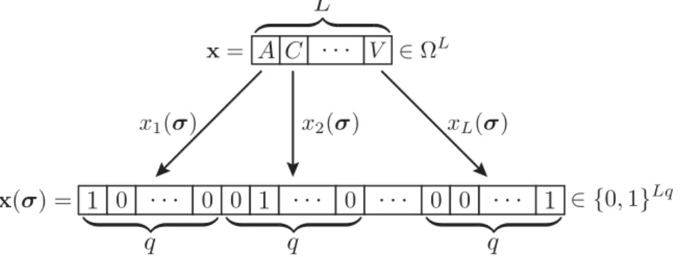
To formalize the derivation of the pairwise maximum-entropy probability distribution on categorical variables, we use the approach of [8,30,48] and replace, as depicted inFig 2, each variablexidefined on categorical variables by an indicator function of the amino acids₂Ω, 1s:Ω!{0, 1}q,

xi7!xiðsÞ:1sðxiÞ ¼

1 ifxi¼s;

0 otherwise:

(

This embedding specifies a unique representation of anyL-vector of categorical random variables,x, as a binaryLq-vector,x(σ)with a single non-zero entry in each binaryq-subvector

xi(σ)= (xi(s1),. . .,xi(sq))T2{0,1}q,

x¼ ðx1;. . .;xLÞ

T

2OL_7!1s_xðσ_{Þ ¼ ð}x1ðs1Þ;. . .;xLðsqÞÞ

T

2 f0;1gLq:

Inserting this embedding into the first and second moment constraints, corresponding to Eqs3and4in the continuous variable case, we find their embedded analogues, the single and pairwise marginal probability in positionsiandjfor amino acidss,o,2Ω

hxiðsÞi ¼ X

xðσÞ

PðxðσÞÞxiðsÞ ¼ X

x

Pðxi¼sÞ ¼PiðsÞ;

hxiðsÞxjðoÞi ¼ X

xðσÞ

Pðxðσ_ÞÞxiðsÞxjðoÞ ¼ X

x

Pðxi¼s;xj¼oÞ ¼Pijðs;oÞ

includingPii(s,o) =Pi(s)1s(o) and with the distribution’sfirst moment in each random

vari-able,hyii ¼ X

yPðyÞyiandy= (y1,. . .,yLq) T

2RLq_{. The analogue of the covariance matrix then} becomes a symmetricLq×Lqmatrix of connected correlations whose entriesCij(s,o) =Pij(s,o)

−Pi(s)Pj(o) characterize the dependencies between pairs of variables. In the same way, the

Fig 2. Illustration of binary embedding.The binary embedding1σ:Ω!{0, 1} Lq

maps each vector of categorical random variables,x₂ΩL_{, here represented by a sequence of amino acids from the amino acid}

alphabet (containing the 20 amino acids and one gap element),Ω= {A,C,D,E,F,G,H,I,K,L,M,N,P,Q,R,

S,T,V,W,Y,−}, onto a unique binary representation,x(σ)2{0, 1} Lq

.

sample means translate to the single-site and pair frequency counts overm= 1,. . .,Mdata vectors

xm_{¼ ðx}m 1;. . .;x

m LÞ

T

2OL_,

xiðsÞ ¼

1

M XM

m¼1 xm

i ðsÞ ¼fiðsÞ;

xiðsÞxjðoÞ ¼

1

M XM

m¼1 xm

i ðsÞx m

j ðoÞ ¼fijðs;oÞ:

The pairwise maximum-entropy probability distribution in categorical variables has to ful-fill the normalization constraint,

X

x

Pðx_{Þ ¼}X

xðσÞ

Pðx_ðσ_{ÞÞ ¼}1: ð9Þ

Furthermore, the single and pair constraints, the analogues of Eqs3and4, enforce the resul-ting probability distribution to be compatible with the measured single and pair frequency counts,

PiðsÞ ¼fiðsÞ; Pijðs;oÞ ¼fijðs;oÞ ð10Þ

for eachi,j= 1,. . .,Land amino acidss,o2Ω. As before, we require the probability distribu-tion to maximize the informadistribu-tion entropy,

maximizeS¼ X

x

Pðx_ÞlnPðx_{Þ ¼} X

xðσÞ

Pðx_ðσ_ÞÞlnPðx_ðσ_ÞÞ: ð11Þ

The corresponding Lagrangian,L_¼L_{ðPðxðσÞÞ;a;βðσÞ;γðσ;ωÞÞ, has the functional form,}

L_{¼Sþaðh1i 1Þ þ}X

L

i¼1 X

s2O

b_iðs_ÞðPiðsÞ fiðsÞÞ þ XL

i;j¼1 X

s;o2O

g_ijðs;o_ÞðPijðs;oÞ fijðs;oÞÞ:

For notational convenience, the Lagrange multipliersβ_i(s) andγ_ij(s,o) are grouped to the

Lq-vectorβðσÞ ¼ ðb_iðsÞÞsi¼21O;...;Land theLq×Lq-matrixγðσ;ωÞ ¼ ðgijðs;oÞÞ

s;o2O

i;j¼1;...;L,

respec-tively. The Lagrangian’s stationary point, found as the solution of @L

@PðxðσÞÞ¼0, determines the

pairwise maximum-entropy probability distribution in categorical variables [30,49],

Pðx_ðσ_Þ;β;γ_{Þ ¼} 1 Zexp

XL

i¼1 X

s2O

b_iðsÞxiðsÞ þ XL

i;j¼1 X

s;o2O

g_ijðs;oÞxiðsÞxjðoÞ !

ð12Þ

with normalization by the partition function,Zexp(1−α). Note that distributionEq 12is of

the same functional form asEq 8but with binary random variablesx(σ)₂{0,1}Lqinstead of continuous onesx₂RL_{. At this point, we introduce the reduced parameter set,hi(s): =β}

i(s)+

γ_ii(s,s) andeij(s,o): = 2γ_ij(s,o) fori<j, using the symmetry of the Lagrange multipliers,

γ_ij(s,o): =γ_ji(o,s), and thatxi(s)xi(o) = 1 if and only ifs=o. For a given sequence (z1,. . .,

zL)2ΩLsumming over all non-zero elements, (x1(z1) = 1,. . .,xL(zL) = 1) or equivalently (x1=

z1,. . .,xL=zL) then yields the probability assigned to the sequence of interest,

Pðz1;. . .;zLÞ

1

Zexp XL

i¼1

hiðziÞ þ X

1i<jL eijðzi;zjÞ

!

: ð13Þ

Gauge fixing

In contrast to the continuous variable case in which the number of constraints naturally matches the number of unknown parameters, the case of categorical variables has dependencies due to1_¼X

s2OPiðsÞfor eachi= 1,. . .,LandPiðsÞ ¼

X

o2OPijðs;oÞfor eachi,j= 1,. . .,L ands₂Ω. This results in at mostLðL1Þ

2 ðq1Þ 2

þLðq1_Þindependent constraints compared toLðL1Þ

2 q

2_{þLqfree parameters to be estimated. To ensure the uniqueness of the inferred}

parameters in defining the Hamiltonian,H_ðx

1;. . .;xLÞ ¼ X

i<jeijðxi;xjÞ X

ihiðxiÞ, and, by

implication, the probability distribution, one has to reduce the number of independent parame-ters such that these match the number of independent constraints. For this purpose, so-called gaugefixing [5] has been proposed, which can be realized in different ways. For example, the authors of [6,7] set the parameters corresponding to the last amino acid in the alphabet,sq, to

zero, i.e.,eij(s_q,) =eij(,s_q) = 0 andhi(s_q) = 0 for 1i<jL, resulting in rows and columns of zeros at the end of eachq q-block of theLq × Lqcoupling matrix. Alternatively, the authors of [5] introduce a zero-sum gauge,X

seijðs;oÞ ¼

X

seijðo

0_{;sÞ ¼0and}X

shiðsÞ ¼ 0for each 1i<jLando,o₂Ω. However, different gaugefixings are not equally efficient for the purpose of protein contact prediction. The zero-sum gauge is the parameterfixing that minimizes the sum of squares of the pairwise parameters in the HamiltonianH_,

X

s;oeijðs;oÞ

2

, which makes it the suitable choice when using non-gauge invariant scoring

functions, such as the (average product-corrected) Frobenius norm [5,50] (see section“Scoring Functions”). Moreover, no gaugefixing is required when combining the strictly convexℓ1_{- or} ℓ2_{-regularizer with negative loglikelihood minimization; here the regularizer selects for a unique}

representation among all parametrizations of the optimal distribution [32,51]. However, to additionally minimize the Frobenius norm of the pairwise interactions, [51] changed the obtained full parameter set from regularized inference with plmDCA to zero-sum gauge by,

eijðs;oÞ7!eijðs;oÞ 1q X

s0eijðs0;oÞ 1q X

o0eijðs;o0Þ þq12 X

s0;o0eijðs0;o0Þ, whereqdenotes

the length of the alphabet.

Network interpretation

The derived pairwise maximum-entropy distributions in Eqs13or12and8specify an undi-rected graphical model or Markov random field [34,41]. In particular, a graphical model repre-sents a probability distribution in terms of a graph that consists of a node and an edge set. Edges characterize the dependence structure between nodes and a missing edge then corre-sponds toconditional independencegiven the remaining random variables. For continuous, real-valued variables, the maximum-entropy distribution with first and second moment con-straints is multivariate Gaussian, which will be demonstrated in the next section. Its depen-dency structure is represented by a graphical Gaussian model (GGM) in which a missing edge,

γij= 0, corresponds to conditional independence between the random variablesxiandxj(given

the remaining ones), and is further specified by a zero entry in the corresponding inverse covariance matrix, (C−1₎

ij= 0.

In the next section, we describe how the dependency structure of the graph is inferred.

Inference of Interactions

methods to estimate these parameters that have recently been used in the context of protein contact prediction. Those are (1) for continuous variables, the exact closed-form solution which approximates the mean-field result for categorical variables, and (2) three inference methods for categorical variables based on the maximum-likelihood methodology: the stochas-tic maximum likelihood, the approximation by pseudo-likelihood maximization, and finally, the sparse maximum-likelihood solution.

Closed-Form Solution for Continuous Variables

The simplest approach to extract the unknown Lagrange multipliersα,β= (βi), andγ= (γij)

fromP(x) exactly is to use basic integration properties of the continuous random variablesxiin the constraints Eqs3–5. For this purpose, we rewrite the exponent of the pairwise maximum-entropy probability distributionEq 8,

Pðx;β;~γ_{Þ ¼}1 Zexp β

T

x1

2x T_γ~x

¼1

Zexp

1 2β

T_~γ1_β

1

2ðxγ~

1_β

ÞTγ~_ðxγ~1_β Þ

;

where we use the replacementγ~:¼ 2γand requireγ~to be positive definite (which is equiva-lent toγbeing negative definite), i.e.,xTγ~x>0for anyx6¼0, which makes its inverse~γ1_¼ 1

2γ

1_well-de

fined. As already discussed, this is a sufficient condition on the integrals in Eqs 3–6to befinite. For notational convenience, we define the shifted variablez_{¼ ð}z1;. . .;zLÞ

T :_¼

xγ~1_βorx i ¼ziþ

XL

j¼1ðγ~ 1_Þ

ijbjand accordingly, the maximum-entropy probability

dis-tribution becomes

PðxÞ ¼ 1_~

Zexp

1 2ðxγ~

1_βÞT_γ~ðxγ~1_βÞ

1_~

Ze 1

2zTγ~z ð14Þ

with the normalization constant_Z~_{¼exp 1a}1 2β

T_γ~1_β

. The normalization conditionEq 3in the new variable is,

1_¼

ð

x

Pðx_Þdx1

~

Z ð

z e1

2zTγ~zd_z ð15Þ

and the linear shift does not affect the integral when integrated overRL_{yielding for the}

nor-malization constant,_Z~_¼

ð

z e1

2zT~γzdz. Furthermore, thefirst-order constraintEq 4becomes

for eachi= 1,. . .,L,

hxii ¼ ð

x

Pðx_Þxidx

1 ~

Z ð

z e1

2zT~γz z iþ

XL

j¼1 ðγ~1

Þijbj !

dz_¼X

L

j¼1 ðγ~1

Þijbj

and we used the point symmetry of the integrand then,

ð

z e1

2zT~γzz

idz¼0in eachi= 1,. . .,L.

Analogously, wefind for the second moment, determining the correlations for each index pair

i,j= 1,. . .,L,

hxixji ¼ ð

x

Pðx_Þxixjdx

1 ~

Z ð

z e1

2zT~γzðz

i hxiiÞðzj hxjiÞdz¼ hzizji þ hxiihxji;

on this, the covariance is found as,

Cij¼ hxixji hxiihxji hzizji:

Finally, the termhzizjiis solved using a spectral decomposition of the symmetric and posi-tive-definite matrixγ~as sum over products of its eigenvectorsv1,. . .,v_Land real-valued and

pos-itive eigenvaluesλ1,. . .,λL,γ~¼ XL

k¼1lkvkv

T

k. The eigenvectors form a basis ofR

L_{and assign}

new coordinates,y1,. . .,yL, toz_¼XL

k¼1ykvk, which allows writing of the exponenthzizjias

zTγ~z¼XL_k¼1l_ky2

k. The covariance betweenxiandxjthen reads as (Bishop [52], p. 83)

hzizji ¼

1 ~

Z XL

l;n¼1

ðvlÞiðvnÞj ð

y

exp 1₂X

L

k¼1 l_ky2

k !

ylyndy¼ XL

k¼1

1

l_kðvkÞiðvkÞj ðγ~ 1

Þij

with solutionCij¼ ðγ~ 1_Þ

ijorðC 1_Þ

ij¼ ð~γÞij¼ 2gij. Taken together, the Lagrange multipliers βandγare specified in terms of the mean,hx_i, and the inverse covariance matrix (also known as the precision or concentration matrix),C−1_,

β_¼C1

hx_i; γ_¼ 1

2γ~¼ 1 2C

1_:

ð16Þ

As a consequence, the real-valued maximum-entropy distributionEq 14for given first and second moments is found as themultivariate Gaussian distribution,which is determined by the meanhxiand the covariance matrixC,

Pðx;_hxi;CÞ ¼ ð2pÞL=2

detðCÞ1=2

exp 1

2ðx hxiÞ T

C1

ðx hxiÞ

ð17Þ

and we refer to [52] for the derivation of the normalization factor. The initial requirement of ~

γ¼ 2γto be positive definite results in a positive-definite covariance matrixC, a necessary condition for the Gaussian density to be well defined. In summary, the multivariate Gaussian distribution maximizes the entropy among all probability distributions of continuous variables with specifiedfirst and second moments. The pair interaction strength is now evaluated by the already introduced partial correlation coefficient betweenxiandxjgiven the remaining vari-ables {xr}r2{1,. . .,L}\{i,j},

r_{ijf1;...;Lgnfi;jg} gij ffiffiffiffiffiffiffiffi g_iig_jj

p ¼

ðC1_Þ ij ffiffiffiffiffiffiffiffiffiffiffiffiffiffiffiffiffiffiffiffiffiffiffiffiffiffi

ðC1_Þ iiðC

1_Þ jj

q if i6¼j;

1 if i¼j:

ð18Þ

8 > > < > > :

Data integration

In biological datasets as used to study gene association, the number of measurements,M, is typically smaller than the number of observables,L, i.e.,M<Lin our terminology.

Conse-quently, the empirical covariance matrix,_C^_¼ 1 M

XM

m¼1ðx

m_xÞðxm_xÞT

matrix,C1_C1

d;l,

C1

d;l ¼arg max

Y_pos:definite;

symmetric

fln detðY_{Þ traceðC}^Y_{Þ lk}Y_kd

dg ð19Þ

with penalty parameterλ0 andkY_kd d¼

X

i;jj

Y

ijj

d

. Ifλ= 0, we obtain the

maximum-likeli-hood estimate, forδ= 1 andλ>0 theℓ1_{-regularized (sparse) maximum-likelihood solution}

that selects for sparsity [53,54], and forδ= 2 andλ>0 theℓ2_{-regularized maximum-likelihood}

solution that favors small absolute values in the entries of the selected inverse covariance matrix [55]. Forδ= 1 andλ>0, the method is called LASSO, forδ= 2 andλ>0, ridge regres-sion. Alternatively, regularization can be directly applied to the covariance matrix, e.g., by shrinkage [17,56].

Solution for categorical variables

An ad hoc ansatz to extract the pairwise parameters in the categorical variables case (12) is to extend the binary variablexðσ_{Þ ¼ ð}xiðskÞÞik 2 f0;1g

Lðq1Þ_{to a continuous one,}

y= (yj)j2RL(q−1),

and replace the sums in the distribution and the momentshiby integrals. The extended binary maximum-entropy distributionEq 12is then approximated by theLq-dimensional multivariate Gaussian with inherited analogues of the meanhyi ¼ ðfiðskÞÞik2R

Lðq1Þ_{and the empirical}

covariance matrix_C^_{ðσ;ωÞ ¼ ðC}^

ijðsk;slÞÞi;j;k;l 2R

Lðq1Þ Lðq1Þ_{whose elementsC^}

ijðs;oÞ ¼ fijðs;oÞ fiðsÞfjðoÞare characterizing the pairwise dependency structure. The gaugefixing

results in setting the preassigned entries referring to the last amino acid in the mean vector and the covariance matrix to zero, which reduces the model’s dimension fromLqtoL(q−1); other-wise the unregularized covariance matrix would always be non-invertible. Typically, the single and pair frequency counts are reweighted and regularized by pseudocounts (see section “Sequence data preprocessing”) to additionally ensure that_C^_{ðσ;ωÞis invertible. Final} applica-tion of the closed-form soluapplica-tion for continuous variablesEq 16to the extended binary variables forC1

ðσ;ω_Þ C^1

ðσ;ω_Þyields the so-called mean-field (MF) approximation [48],

gMF

ij ðs;oÞ ¼

1 2ðC

1

Þijðs;oÞ

)

MF

ij ðs;oÞ ¼ ðC 1

Þijðs;oÞ ð20Þ

for amino acidss,o2Ωand with restriction to residuesi<jin the latter identity. The same solution has been obtained by [6,7] using a perturbation ansatz to solve theq-state Potts model termed (mean-field) Direct Coupling Analysis (DCA or mfDCA). In Ising models, this result is also known as naïve mean-field approximation [57–59].

The following section is dedicated to maximum likelihood-based inference approaches, which have been presented in the field of protein contact prediction.

Maximum-Likelihood Inference

A well-known approach to estimate the parameters of a model is maximum-likelihood infer-ence. The likelihood is a scalar measure of how likely the model parameters are, given the observed data (Mackay [34], p. 29), and the maximum-likelihood solution denotes the parame-ter set maximizing the likelihood function. For Markov random fields, the maximum-likeli-hood solution is consistent, i.e., recovers the true model parameters in the limit of infinite data (Koller and Friedman [32], p. 949). In particular, for a pairwise model with parametersh_ðσ_{Þ ¼}

ðhiðsÞÞ

s2O

i¼1;...;Landeðσ;ωÞ ¼ ðeijðs;oÞÞ

s;o2O

ω)|x1,. . .,xM) given observed data,x1,. . .,xM2ΩL,which are assumed to be independent and identically distributed (iid), as

lðh_ðσ_Þ;e_ðσ;ω_Þjx1;. . .;xMÞ ¼Y

M

m¼1

Pðxm;h_ðσ_Þ;e_ðσ;ω_ÞÞ: ð21Þ

The estimates of the model parameters are then obtained as the maximizer of l or, using the monotonicity of the logarithm, the minimizer of ln l,

fhML_ðσ_Þ;eML_{ðσ;ωÞg ¼arg max}

hðsÞ;eðs;oÞ

lðh_ðσ_Þ;e_ðσ;ω_ÞÞ arg min

hðsÞ;eðs;oÞ

lnlðh_ðσ_Þ;e_ðσ;ω_ÞÞ:

When we specify the maximum-entropy distributionEq 13as model distribution, the then-concave loglikelihood [32] becomes

lnlðh_ðσÞ;e_{ðσ;ωÞÞ ¼}X M

m¼1

lnPðxm_{;hðσÞ;eðσ;ωÞÞ}

¼ M lnZX

L

i¼1 X

s

hiðsÞfiðsÞ X

1i<jL X

s;o

eijðs;oÞfijðs;oÞ

" #

:

ð22Þ

The maximum-likelihood solution is found by taking the derivatives ofEq 22with respect to the model parametershi(s) andeij(s,o) and setting to zero,

@ @hiðsÞ

lnl ¼ M @

@hiðsÞ

lnZ

j

fh_ðσÞ;e_ðσ;ωÞgfið sÞ

¼0;

@ @eijðs;oÞ

lnl ¼ M @

@eijðs;oÞ

lnZ

j

fh_ðσÞ;e_ðσ;ωÞg fijðs;oÞ

" #

¼0:

ð23Þ

The partial derivatives of the partition function,

Z¼X_ðx1;...;x

LÞexp

X

ihiðxiÞ þ X

i<jeijðxi;xjÞ

, follow the well-known identities

@ @hiðsÞ

lnZ

j

fh_ðσÞ;e_ðσ;ωÞg¼

1

Z@hiðsÞZ

j

fh_ðσÞ;e_ðσ;ωÞg¼Pið

s;h_ðσ_Þ;e_ðσ;ω_ÞÞ;

@ @eijðs;oÞ

lnZ

j

fh_ðσÞ;e_ðσ;ωÞg¼

1

Z@eijðs;oÞZ

j

fh_ðσÞ;e_ðσ;ωÞg¼Pijð

s;o;h_ðσ_Þ;e_ðσ;ω_ÞÞ:

The maximizing parameters,hML_ðσ_{Þ ¼ ð}hML

i ðsÞÞ

s2O

i¼1;...;Lande

ML_{ðσ;ωÞ ¼ ðe}ML

ij ðs;oÞÞ

s;o2O

1i<jL,

are those matching the distribution’s single and pair marginal probabilities with the empirical single and pair frequency counts,

Piðs;h

ML

ðσ_Þ;eML_{ðσ;ωÞÞ ¼f}

iðsÞ; Pijðs;o;h

ML

ðσ_Þ;eML_{ðσ;ωÞÞ ¼f}

ijðs;oÞ

Based on the maximum-likelihood principle, we present three solution approaches in the remainder of this section.

Stochastic maximum likelihood

The maximum-likelihood solution is typically inaccessible for models of categorical variables due to the computational complexity of estimating the partition functionZwhich involves a sum over all possible states and grows exponentially with the size of the system [3,61]. Lapedes et al. [30] solvedEq 22by likelihood maximization on sampled subsets using the Metropolis– Hastings algorithm [32,34]. In particular, the likelihood is maximized iteratively by following the steepest ascent of the loglikelihood function lnlusingEq 23. In each maximization step, the parametershðkÞi ðsÞande

ðkÞ

ij ðs;oÞare changed in proportion to the gradient of lnland

scaled by the constant step sizeε>0,

D_hðkÞ_{i ðsÞ ¼}ε @

@hiðsÞ

lnl

j

fhðkÞ_ðσÞ;eðkÞ_ðσ;ωÞg/fið

sÞ Piðs;h

ðkÞ_ðσÞ;eðkÞ_ðσ;ωÞÞ;

D_eðkÞ

ij ðs;oÞ ¼ε

@ @eijðs;oÞ

lnl

j

fhðkÞ_ðσÞ;eðkÞ_ðσ;ωÞg/fijð

s;o_Þ Pijðs;o;h ðkÞ

ðσ_Þ;eðkÞ_ðσ;ω_ÞÞ

until convergence is reached as the differencesD_hðkÞ_{i ðs;oÞ:¼hi}ðkþ1Þ_{ðs;oÞ h}ðkÞ_{i ðs;oÞ,}

i= 1,. . .,L, andD_eðkÞ_{ij ðs;oÞ}:_¼eðkþij 1Þðs;oÞ e ðkÞ

ij ðs;oÞ, 1i<jL, go to zero [30]. The

com-putation of the marginals requires summing over 20L_{states and is, for example, estimated by}

Monte-Carlo sampling. As the likelihood is concave, there are no local maxima and the maxi-mum-likelihood parameters are obtained in the limitk! 1,

fhML_ðσ_Þ;eML_{ðσ;ωÞg ¼lim}

k!1f

hðkÞ_ðσ_Þ;eðkÞ_ðσ;ωÞg

orD_hðkÞ_{i ðs;oÞ !0fori= 1,. . .,Land}D_eðkÞ_{ij ðs;oÞ !0for 1i<jLands,o2Ω\ {sq}, a} subset ofΩcontainingq−1 elements to account for gaugefixing.

Pseudo-likelihood maximization

Besag [62] introduced the pseudo-likelihood as approximation to the likelihood function in which the global partition function is replaced by computationally tractable local estimates. The pseudo-likelihood inherits the concavity from the likelihood and yields the exact maxi-mum-likelihood parameter in the limit of infinite data for Gaussian Markov random fields [41,62], but not in general [63]. Applications of this approximation to non-continuous categor-ical variables have been studied, for instance, in sparse inference of Ising models [64] but may lead to results that differ from the maximum-likelihood estimate. In this approach, the proba-bility of them-th observation,xm, is approximated by the product of the conditional probabili-ties ofxr¼xmr given observations in the remaining variables

x_nr:¼ ðx1;. . .;xr1;xrþ1;. . .;xLÞ

T

2OL1_[51],

Pðxm;h_ðσÞ;e_{ðσ;ωÞÞ ’}Y L

r¼1

Pðxr ¼x m

r jxnr ¼x m

Each factor is of the following analytical form,

Pðxr ¼x m

rjxnr ¼x m

nr;hðσÞ;eðσ;ωÞÞ ¼

exp hrðxmrÞ þ X

j6¼r

erjðxmr;xjmÞ !

X

s

exp hrðsÞ þ X

j6¼r

erjðs;xjmÞ !;

which only depends on the unknown parameters (eij(s,o))i6¼r,j6¼rand (hi(s))i6¼rand makes the

computation of the pseudo-likelihood tractable. Note, we treateij(s,o) =eji(o,s) andeii(,) = 0. By this approximation, the loglikelihoodEq 21becomes the pseudo-loglikelihood,

lnlPLðhðσÞ;eðσ;ωÞÞ:¼

XM

m¼1 XL

r¼1

lnPðxr ¼x m

rjxnr ¼xmnr;hðσÞ;eðσ;ωÞÞ:

In the final formulation of the pseudo-likelihood maximization (PLM) problem, anℓ2

-regu-larizer is added to select for small absolute values of the inferred parameters,

fhPLM_ðσ_Þ;ePLM_ðσ;ω_{Þg ¼}arg min

h_ðσÞ;e_ðσ;ωÞ

flnlPLðhðσÞ;eðσ;ωÞÞ þlhkhðσÞk 2

2 þlekeðσ;ωÞk 2 2g;

whereλh,λe>0 adjust the complexity of problem and are selected in a consistent manner across

different protein families to avoid overfitting. This approach has been presented (with scaling of the pseudo-loglikelihood by 1

Meffwmto include sequence weighting, see section“Sequence data

preprocessing”) by [51] under the name plmDCA (PseudoLikelihood Maximization Direct Cou-pling Analysis) and has shown performance improvements compared to the mean-field approxi-mationEq 20. Another inference method based on the pseudolikelihood maximization but including prior knowledge in terms of secondary structure and information on pairs likely to be in contact is Gremlin (Generative REgularized ModeLs of proteINs) [65–67].

Sparse maximum likelihood

Similar to the derivation of the mean-field result (20), Jones et al. [8] approximatedEq 12by a multivariate Gaussian and accessed the elements of the inverse covariance matrix by a maxi-mum-likelihood inference under sparsity constraint [54,68,69]. The corresponding method has been called Psicov (Protein Sparse Inverse COVariance). The validity of this approach to solve the sparse maximum-likelihood problem in binary systems such as Ising models has been dem-onstrated by [69], followed by consistency studies [70]. In particular, the Psicov method infers the sparse maximum-likelihood estimate of the inverse covariance matrixEq 19forδ= 1 using the analogue of the empirical covariance matrix derived from the observed amino acid frequen-cies,_C^_{ðσ;ωÞ. Its elementsC}^

ijðs;oÞ ¼fijðs;oÞ fiðsÞfjðoÞ, the empirical connected

correla-tions, are preprocessed by reweighting and regularized by pseudocounts and shrinkage. Regularized loglikelihood maximizationEq 19selects a unique representation of the model, i.e., no additional gaugefixing is required. Using identityEq 16on the elements of the sparse maximum-likelihood (SML) estimate of the inverse covariance,C1

1;lðσ;ωÞ, yields the estimates for the Lagrange multipliers,

gSML

ij ðs;oÞ ¼

1 2ðC

1

1;lÞijðs;oÞ

)

SML

ij ðs;oÞ ¼ ðC 1 1;lÞijðs;oÞ

indicesi,j= 1,. . .,Lhave been hypothetically translated to the reduced parameter formulation

eij(s,o) for 1i<jL.

Sequence data preprocessing

The study of residue–residue co-evolution is based on data from multiple sequence alignments, which represent sampling from the evolutionary record of a protein family. Multiple sequence alignments from currently existing sequence databases do not evenly represent the space of evolved sequences as they are subject to acquisition bias towards available species of interest. To account for uneven representation, sequence reweighting has been introduced to lower the contributions of highly similar sequences and assign higher weight to unique ones (see Durbin et al. [44], p. 124 ff.). In particular, the weight of them-th sequence,wm: = 1/km, in the

align-ment {x1,. . .,xM}, can be chosen to be the inverse ofkm:¼ XM

n¼1H XL

i¼11ðx m i ;x

n

iÞ Ly

,

the number of sequencesxmshares more thanθ_{100% of its residues with. Here,}θ_{denotes a}

similarity threshold and is typically chosen as 0.7θ_{0.9,1(a,b) = 1 ifa=band1(a,b) = 0,}

otherwise, andHis the step function withH(y) = 0 ify<0 andH(y) = 1, otherwise. This also provides us with an estimate of the effective number of sequences in the alignment,

Meff :¼

XM

m¼1wm. Additionally, pseudocount regularization with

~

l>0is used to deal with finite sampling bias and to account for underrepresentation [5–8,44,48], resulting in zero entries in_C^_{ðσ;ωÞ, for instance, if a certain amino acid pair is never observed. The use of} pseu-docounts is equivalent to a maximum a posteriori (MAP) estimate under a specific inverse Wishart prior on the covariance matrix [48]. Both preprocessing steps combined yield the reweighted single and pair frequency counts,

fiðsÞ ¼

1

Meffþl~ ~

l qþ

XM

m¼1 wmx

m i ðsÞ

!

; fijðs;oÞ ¼

1

Meffþ~l ~

l q2þ

XM

m¼1 wmx

m i ðsÞx

m j ðoÞ

!

;

in residuesi,j= 1,. . .,Land for amino acidss,o₂Ω. Ideally for maximum-likelihood inference, the random variables are assumed to be independent and identically distributed. However, this is typically violated in realistic sequence data due to phylogenetic and sequencing bias, and the reweighting presented here does not necessarily solve this problem.

Scoring Functions for the Pairwise Interaction Strengths

For pairwise maximum-entropy models of continuous variables, the natural scoring function for the interaction strength between two variablesxiandxj, given the inferred inverse covari-ance matrix, is the partial correlationEq 18. However, for categorical variables, the situation is more complicated, and there are several alternative choices of scoring functions. Requirements on the scoring function are that it has to account for the chosen gauge and, in the case of pro-tein contact prediction, evaluate the coupling strength between two residuesiandj summa-rized across all possibleq2amino acids pairs. The highest scoring residue pair is, for instance, used to predict the 3-D structure of the protein of interest. For this purpose, the direct informa-tion, defined as the mutual information applied toPdir

ij ðs;oÞ ¼ 1

Zijexpðeijðs;oÞ þ

~

hiðsÞ þ

~

hjðoÞÞinstead offij(s,o),

DI_ij¼ X

s;o2O

Pdirij ðs;oÞln Pdir

ij ðs;oÞ fiðsÞfjðoÞ !

;

has been introduced [5]. InPdir

(reweighted and regularized) single-site frequency counts,fi(s) andfj(o), andZijsuch that the sum over all pairs (i,j) with 1i<jLis normalized to 1. The direct information is invariant under gauge changes of the HamiltonianH_{, which means that any suitable gauge choice results} in the same scoring values. As an alternative measure of the interaction strength for a particular pair (i,j), the Frobenius norm of the 21×21-submatrices of (eij(s,o))s,ohas been used,

keijkF¼

X

s;o2O

eijðs;oÞ 2

!1=2 :

However, this expression is not gauge-invariant [5]. In this context, the notation witheij(s,

o), which refers to indices restricted toi<j, is extended and treated such thateij(s,o) =eji(o,

s) andeij(,) = 0; then ||eij||F= ||eji||Fand ||eii||F= 0. In order to correct for phylogenetic biases in the identification of co-evolved residues, Dunn et al. [27] introduced the average product correction (APC). It has been originally used in combination with the mutual information but was recently combined with theℓ1_{-norm [8] and the Frobenius/}ℓ2_{-norm [51] and is derived}

from the averages over rows and columns of the corresponding norm of the matrix of theeij

parameters. In this formulation, the pair scoring function is

APCFNij¼keijkF

ke_ikFkejkF

kekF

ð24Þ

foreij-parametersfixed by zero-sum gauge and with the means over the non-zero elements in

row, column and full matrix,ke_ikF:¼L11 XL

j¼1keijkF,kejkF:¼ 1 L1

XL

i¼1keijkFand kekF:¼

1 LðL1Þ

XL

i;j¼1keijkF, respectively. Alternatively, the average product-corrected

ℓ1_-norm

applied to the 20×20-submatrices of the estimated inverse covariance matrix, in which contri-butions from gaps are ignored, has been introduced by the authors of [8] as the Psicov-score. Using the average product correction, the authors of [51] showed for interaction parameters inferred by the mean-field approximation that scoring with the average product-corrected Fro-benius norm increased the precision of the predicted contacts compared to scoring with the DI-score. The practical consequence of the choice of scoring method depends on the dataset and the parameter inference method.

Discussion of Results, Improvements, and Applications

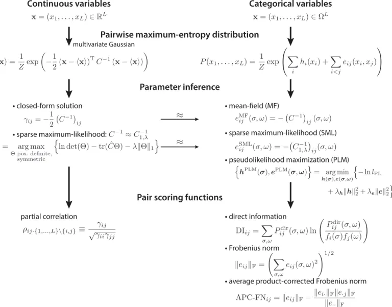
Maximum entropy-based inference methods can help in estimating interactions underlying biological data. This class of models, combined with suitable methods for inferring their numerical parameters, has been shown to reveal—to a reasonable approximation—the direct interactions in many biological applications, such as gene expression or protein residue—resi-due coevolution studies. In this review, we have presented maximum-entropy models for the continuous and categorical random variable case. Both approaches can be integrated into a framework, which allows the use of solutions obtained for continuous variables as approxima-tions for the categorical random variable case (Fig 3).

as the result of extraordinary advances in sequencing technology. The quality of existing meth-ods can be improved by careful refinement of sequence alignments in terms of cutoffs and gaps or by attaching optimized weights to each of the data sequences. Alternatively, one could try to improve the existing model frameworks by accounting for phylogenetic progression [27,49,72] and finite sampling biases.

The advancement of inference methods for biological datasets could help solve many inter-esting biological problems, such as protein design or the analysis of multi-gene effects in relat-ing variants to phenotypic changes as well as multi-genic traits [73,74]. The methods presented here could help reduce the parameter space of genome-wide association studies to first approx-imation. In particular, we envision the following applications: (1) in the disease context, co-evolution studies of oncogenic events, for example copy number alterations, mutations, fusions

Fig 3. Scheme of pairwise maximum-entropy probability models.The maximum-entropy probability distribution with pairwise constraints for continuous random variables is the multivariate Gaussian distribution (left column). For the maximum-entropy probability distribution in the categorical variable case (right column), various approximative solutions exist, e.g., the mean-field, the sparse maximum-likelihood, and the pseudolikelihood maximization solution. The mean-field and the sparse maximum-likelihood result can be derived from the Gaussian approximation of binarized categorical variables (thin arrow). Pair scoring functions for the continuous case are the partial correlations (left column). For the categorical variable case, the direct information, the Frobenius norm, and the average product-corrected Frobenius norm are used to score pair couplings from the inferred parameters (right column).

and alternative splicing, can be used to derive direct co-evolution signatures of cancer from available data, such as The Cancer Genome Atlas (TCGA); (2)de novodesign of protein sequences as, for example, described in [65,75] for the WW domain using design rules based on the evolutionary information extracted from the multiple sequence alignment; and (3) develop quantitative models of protein fitness computed from sequence information.

In general, in a complex biological system, it is often useful for descriptive and predictive purposes to derive the interactions that define the properties of the system. With the methods presented here and available software (Table 1), our goal is not only to describe how to infer these interactions but also to highlight tools for the prediction and redesign of properties of biological systems.

Acknowledgments

We thank Theofanis Karaletsos, Sikander Hayat, Stephanie Hyland, Quaid Morris, Deb Bemis, Linus Schumacher, John Ingraham, Arman Aksoy, Julia Vogt, Thomas Hopf, Andrea Pagnani, and Torsten Groß for insightful discussions.

References

1. Lezon TR, Banavar JR, Cieplak M, Maritan A, Fedoroff NV. Using the principle of entropy maximization to infer genetic interaction networks from gene expression patterns. Proceedings of the National Acad-emy of Sciences of the United States of America. 2006; 103(50):19033–19038. PMID:17138668

2. Locasale JW, Wolf-Yadlin A. Maximum entropy reconstructions of dynamic signaling networks from quantitative proteomics data. PloS one. 2009; 4(8):e6522. doi:10.1371/journal.pone.0006522PMID:

19707567

3. Schneidman E, Berry II MJ, Segev R, Bialek W. Weak pairwise correlations imply strongly correlated network states in a neural population. Nature. 2006; 440:1007–1012. PMID:16625187

4. Tang A, Jackson D, Hobbs J, Chen W, Smith JL, Patel H, et al. A maximum entropy model applied to spatial and temporal correlations from cortical networks in vitro. The Journal of Neuroscience. 2008; 28 (2):505–518. doi:10.1523/JNEUROSCI.3359-07.2008PMID:18184793

5. Weigt M, White RA, Szurmant H, Hoch JA, Hwa T. Identification of direct residue contacts in protein—

protein interaction by message passing. Proceedings of the National Academy of Sciences of the United States of America. 2009; 106(1):67–72. doi:10.1073/pnas.0805923106PMID:19116270

6. Marks DS, Colwell LJ, Sheridan R, Hopf TA, Pagnani A, Zecchina R, et al. Protein 3D Structure Com-puted from Evolutionary Sequence Variation. PLoS One. 2011; 6(12):e28766. doi:10.1371/journal.

pone.0028766PMID:22163331

7. Morcos F, Pagnani A, Lunt B, Bertolino A, Marks D, Sander C, et al. Direct-coupling analysis of residue co-evolution captures native contacts across many protein families. Proceedings of the National Acad-emy of Sciences of the United States of America. 2011; 108:E1293–E1301. doi:10.1073/pnas.

1111471108PMID:22106262

8. Jones DT, Buchan DWA, Cozzetto D, Pontil M. PSICOV: precise structural contact prediction using sparse inverse covariance estimation on large multiple sequence alignments. Bioinformatics. 2012; 28 (2):184–190. doi:10.1093/bioinformatics/btr638PMID:22101153

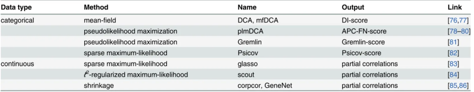
Table 1. Overview of software tools to infer pairwise interactions from datasets in continuous or categorical variables with maximum-entropy/ GGM-based methods.

Data type Method Name Output Link

categorical mean-field DCA, mfDCA DI-score [76,77]

pseudolikelihood maximization plmDCA APC-FN-score [78–80]

pseudolikelihood maximization Gremlin Gremlin-score [81]

sparse maximum-likelihood Psicov Psicov-score [82]

continuous sparse maximum-likelihood glasso partial correlations [83]

ℓ2_{-regularized maximum-likelihood scout partial correlations [84]}

shrinkage corpcor, GeneNet partial correlations [85,86]

9. Stephens GJ, Bialek W. Statistical mechanics of letters in words. Physical Review E. 2010; 81 (6):066119.

10. Bialek W, Cavagna A, Giardina I, Mora T, Silvestri E, Viale M, et al. Statistical mechanics for natural flocks of birds. Proceedings of the National Academy of Sciences. 2012; 109(13):4786–4791.

11. Wood K, Nishida S, Sontag ED, Cluzel P. Mechanism-independent method for predicting response to multidrug combinations in bacteria. Proceedings of the National Academy of Sciences of the United States of America. 2012; 109(30):12254–12259. doi:10.1073/pnas.1201281109PMID:22773816

12. Whittaker J. Graphical models in applied multivariate statistics. Wiley Publishing; 2009.

13. Lauritzen SL. Graphical models. Oxford: Oxford University Press; 1996.

14. Butte AJ, Kohane IS. Unsupervised knowledge discovery in medical databases using relevance net-works. In: Proceedings of the AMIA Symposium. American Medical Informatics Association; 1999. p. 711–715.

15. Toh H, Horimoto K. Inference of a genetic network by a combined approach of cluster analysis and graphical Gaussian modeling. Bioinformatics. 2002; 18(2):287–297. PMID:11847076

16. Dobra A, Hans C, Jones B, Nevins JR, Yao G, West M. Sparse graphical models for exploring gene expression data. Journal of Multivariate Analysis. 2004; 90(1):196–212.

17. Schäfer J, Strimmer K. A shrinkage approach to large-scale covariance matrix estimation and implica-tions for functional genomics. Statistical applicaimplica-tions in genetics and molecular biology. 2005; 4(1):1–

32.

18. Roudi Y, Nirenberg S, Latham PE. Pairwise maximum entropy models for studying large biological sys-tems: when they can work and when they can’t. PLoS Computational Biology. 2009; 5(5):e1000380.

doi:10.1371/journal.pcbi.1000380PMID:19424487

19. Cramér H. Mathematical methods of statistics. vol. 9. Princeton university press; 1999.

20. Guttman L. A note on the derivation of formulae for multiple and partial correlation. The Annals of Math-ematical Statistics. 1938; 9(4):305–308.

21. Krumsiek J, Suhre K, Illig T, Adamski J, Theis FJ. Gaussian graphical modeling reconstructs pathway reactions from high-throughput metabolomics data. BMC Systems Biology. 2011; 5(1):21.

22. Giraud BG and Heumann, John M and Lapedes, Alan S. Superadditive correlation. Physical Review E. 1999; 59(5):4983–4991.

23. Neher E. How frequent are correlated changes in families of protein sequences? Proceedings of the National Academy of Sciences of the United States of America. 1994; 91(1):98–102. PMID:8278414

24. Göbel U, Sander C, Schneider R, Valencia A. Correlated mutations and residue contacts in proteins. Proteins. 1994; 18(4):309–317. PMID:8208723

25. Taylor WR, Hatrick K. Compensating changes in protein multiple sequence alignments. Protein Engi-neering. 1994; 7(3):341–348. PMID:8177883

26. Shindyalov IN and Kolchanov NA and Sander C. Can three-dimensional contacts in protein structures be predicted by analysis of correlated mutations? Protein Engineering. 1994; 7(3):349–358. PMID:

8177884

27. Dunn SD, Wahl LM, Gloor GB. Mutual information without the influence of phylogeny or entropy dramat-ically improves residue contact prediction. Bioinformatics. 2008; 24(3):333–340. PMID:18057019

28. Burger L, Van Nimwegen E. Disentangling direct from indirect co-evolution of residues in protein align-ments. PLoS computational biology. 2010; 6(1):e1000633. doi:10.1371/journal.pcbi.1000633PMID:

20052271

29. Atchley WR, Wollenberg KR, Fitch WM, Terhalle W, Dress AW. Correlations among amino acid sites in bHLH protein domains: an information theoretic analysis. Molecular biology and evolution. 2000; 17 (1):164–178. PMID:10666716

30. Lapedes A, Giraud B, Jarzynski C. Using Sequence Alignments to Predict Protein Structure and Stabil-ity With High Accuracy. eprint arXiv:12072484. 2002;.

31. Ciriello G, Miller ML, Aksoy BA, Senbabaoglu Y, Schultz N, Sander C. Emerging landscape of onco-genic signatures across human cancers. Nature genetics. 2013; 45(10):1127–1133. doi:10.1038/ng. 2762PMID:24071851

32. Koller D, Friedman N. Probabilistic graphical models: principles and techniques. MIT press; 2009.

33. Mead LR, Papanicolaou N. Maximum entropy in the problem of moments. Journal of Mathematical Physics. 1984; 25:2404–2417.

34. MacKay DJ. Information theory, inference and learning algorithms. Cambridge university press; 2003.

36. Agmon N, Alhassid Y, Levine RD. An algorithm for finding the distribution of maximal entropy. Journal of Computational Physics. 1979; 30(2):250–258.

37. Shannon CE. A Mathematical Theory of Communication. Bell system technical journal. 1948; 27 (3):379–423.

38. Jaynes ET. Information Theory and Statistical Mechanics. Physical Review. 1957; 106(4):620–630.

39. Jaynes ET. Information Theory and Statistical Mechanics II. Physical Review. 1957; 108(2):171–190.

40. Jaynes ET. Probability theory: the logic of science. Cambridge: Cambridge university press; 2003.

41. Murphy KP. Machine learning: a probabilistic perspective. The MIT Press; 2012.

42. Balescu R. Matter out of Equilibrium. World Scientific; 1997.

43. Goldstein S, Lebowitz JL. On the (Boltzmann) entropy of non-equilibrium systems. Physica D: Nonlin-ear Phenomena. 2004; 193(1):53–66.

44. Durbin R, Eddy SR, Krogh A, Mitchison G. Biological Sequence Analysis: Probabilistic Models of Pro-teins and Nucleic Acids. Cambridge University Press; 1998.

45. Finn RD, Bateman A, Clements J, Coggill P, Eberhardt RY, Eddy SR, et al. Pfam: the protein families database. Nucleic acids research. 2014; 42:D222–D230. doi:10.1093/nar/gkt1223PMID:24288371

46. Remmert M, Biegert A, Hauser A, Söding J. HHblits: lightning-fast iterative protein sequence searching by HMM-HMM alignment. Nature methods. 2012; 9(2):173–175.

47. Finn RD, Clements J, Eddy SR. HMMER web server: interactive sequence similarity searching. Nucleic acids research. 2011;p. gkr367.

48. Baldassi C, Zamparo M, Feinauer C, Procaccini A, Zecchina R, Weigt M, et al. Fast and accurate multi-variate Gaussian modeling of protein families: Predicting residue contacts and protein-interaction part-ners. PloS one. 2014; 9(3):e92721. doi:10.1371/journal.pone.0092721PMID:24663061

49. Lapedes AS, Giraud BG, Liu LC, Stormo GD. A Maximum Entropy Formalism for Disentangling Chains of Correlated Sequence Positions. In: Proceedings of the IMS/AMS International Conference on Statis-tics in Molecular Biology and GeneStatis-tics; 1998. p. 236–256.

50. Santolini M, Mora T, Hakim V. A general pairwise interaction model provides an accurate description of in vivo transcription factor binding sites. PloS one. 2014; 9(6):e99015. doi:10.1371/journal.pone.

0099015PMID:24926895

51. Ekeberg M, Lövkvist C, Lan Y, Weigt M, Aurell E. Improved contact prediction in proteins: Using pseu-dolikelihoods to infer Potts models. Physical Review E. 2013; 87(1):012707.

52. Bishop CM. Pattern recognition and machine learning. New York: Springer-Verlag; 2006.

53. Meinshausen N, Bühlmann P. High-dimensional graphs and variable selection with the lasso. The Annals of Statistics. 2006; 34(3):1436–1462.

54. Friedman J, Hastie T, Tibshirani R. Sparse inverse covariance estimation with the graphical lasso. Bio-statistics. 2008; 9(3):432–441. PMID:18079126

55. Witten DM, Tibshirani R. Covariance-regularized regression and classification for high dimensional problems. Journal of the Royal Statistical Society: Series B (Statistical Methodology). 2009; 71(3):615–

636.

56. Ledoit O, Wolf M. A well-conditioned estimator for large-dimensional covariance matrices. Journal of multivariate analysis. 2004; 88(2):365–411.

57. Kappen HJ, Rodriguez F. Efficient learning in Boltzmann machines using linear response theory. Neu-ral Computation. 1998; 10(5):1137–1156.

58. Tanaka T. Mean-field theory of Boltzmann machine learning. Physical Review E. 1998; 58(2):2302–

2310.

59. Roudi Y, Aurell E, Hertz JA. Statistical physics of pairwise probability models. Frontiers in computa-tional neuroscience. 2009;3. doi:10.3389/neuro.10.003.2009PMID:19242556

60. Wainwright MJ, Jordan MI. Graphical models, exponential families, and variational inference. Founda-tions and Trends in Machine Learning. 2008; 1(1–2):1–305.

61. Broderick T, Dudik M, Tkacik G, Schapire RE, Bialek W. Faster solutions of the inverse pairwise Ising problem. arXiv preprint arXiv:07122437. 2007;.

62. Besag J. Statistical analysis of non-lattice data. The Statistician. 1975; 24(3):179–195.

63. Liang P, Jordan MI. An asymptotic analysis of generative, discriminative, and pseudolikelihood estima-tors. In: Proceedings of the 25th international conference on Machine learning. ACM; 2008. p. 584–

591.