CENTRO DE CIÊNCIAS DEPARTAMENTO DE FÍSICA
PROGRAMA DE PÓS-GRADUAÇÃO EM FÍSICA MESTRADO ACADÊMICO EM FÍSICA
DÉBORA TORRES
PAIRWISE MAXIMUM-ENTROPY MODEL FOR READING FIXATION DATA
PAIRWISE MAXIMUM-ENTROPY MODEL FOR READING FIXATION DATA
Master Thesis presented to the Post-Graduation Course in Physics of the Federal University of Ceará as part of the requisites for obtaining the Degree of Master in Physics.
Advisor: Prof. Dr. José Soares de
An-drade Junior
FORTALEZA
Gerada automaticamente pelo módulo Catalog, mediante os dados fornecidos pelo(a) autor(a)
T644p Torres, Débora.
PAIRWISE MAXIMUM-ENTROPY MODEL FOR READING FIXATION DATA / Débora Torres. – 2018.
53 f. : il. color.
Dissertação (mestrado) – Universidade Federal do Ceará, Centro de Ciências, Programa de Pós-Graduação em Física, Fortaleza, 2018.
Orientação: Prof. Dr. José Soares de Andrade Junior.
1. Eye tracking. 2. Reading. 3. Fixations. 4. Principle of maximum entropy. 5. Inverse statistical problem. I. Título.
PAIRWISE MAXIMUM-ENTROPY MODEL FOR READING FIXATION DATA
Master Thesis presented to the Post-Graduation Course in Physics of the Federal University of Ceará as part of the requisites for obtaining the Degree of Master in Physics.
Aprovada em: 15/06/2018
BANCA EXAMINADORA
Prof. Dr. José Soares de Andrade Junior (Orientador) Universidade Federal do Ceará (UFC)
Prof. Dr. André Auto Moreira Universidade Federal do Ceará (UFC)
I would like to thank my advisor Professor José Soares for letting me be a part of this project and for his guidance and support throughout this journey, as well as Professor André
Moreira, Tatiana Alonso Amor and Wagner Rodrigues de Sena for their valuable assistance and contribution to this work.
To all the fellows of the Complex Systems group for the company and participation in the experiments.
To the UFC Physics department and Graduate program for the constant help and consideration.
Different people may have mixed interests and preferences when reading certain texts as well as
dissimilar capacities to process information. We are interested in knowing if some types of texts induce a correlated reading behaviour among different readers. To study this problem, we run a
reading experiment using high precision eye-tracking equipment that allows us to collect data of gaze times and locations for people reading diverse texts. Based on previous reading behaviour
research, we expect that such information about the fixations will give us some insight about
attention while reading. For the data analysis, we use a pairwise maximum-entropy inference model to examine the relations between the readers’ fixation configurations. In this approach, we
interpret the correlations between these fixation patterns as “interactions" between the readers. A thermodynamic analysis shows that, for meaningful texts, the system is near a critical point,
which suggests that readers correlate their attention behaviour when reading coherent texts.
Pessoas diferentes podem ter interesses e preferências mistos ao ler certos textos, bem como
capacidades diferentes para processar a informação. No presente trabalho, o nosso interesse é investigar se alguns tipos de textos induzem um comportamento de leitura correlacionado
entre diferentes leitores. Para estudar este problema, realizamos um experimento de leitura usando um equipamento de rastreamento ocular de alta precisão que nos permite coletar dados
de tempo e posição no olhar para pessoas que lêem diversos textos. Com base na pesquisa prévia
de comportamento de leitura, esperamos que essas informações sobre as fixações nos dêem algumas pistas sobre a atenção durante a leitura. Para a análise dos dados, usamos um modelo
de inferência de entropia máxima para examinar as relações entre as configurações de fixação dos leitores. Nessa abordagem, interpretamos as correlações entre esses padrões de fixação
como "interações" entre os leitores. Uma análise termodinâmica mostra que, para textos que têm sentido, o sistema está próximo de um ponto crítico, o que sugere que os leitores correlacionam
seu comportamento de atenção ao ler textos coerentes.
Figure 1 – The human eye. . . 19
Figure 2 – The human visual field. . . 19
Figure 3 – Scene perception. . . 20
Figure 4 – Corneal reflection and bright pupil effect. . . 22
Figure 5 – Example of displayed text. . . 23
Figure 6 – Experimental setup. . . 24
Figure 7 – Example of text with words delimited by boxes. . . 25
Figure 8 – Fixation reading pattern. . . 28
Figure 9 – Fixation configuration colormap. . . 29
Figure 10 – Number of fixations on word versus word frequency. . . 30
Figure 11 – Number of fixations on word versus word frequency in semi-logarithmic scale. 30 Figure 12 – Fixation configuration binary colormap. . . 31
Figure 13 – Specific heat curves obtained for the system of fixation configurations of all texts. . . 32
Figure 14 – Mean magnetization for all subjects. . . 33
Figure 15 – Tcversus. hσii. . . 34
Figure 16 – Ci j vs. Ji j. . . 36
Figure 17 – Specific heat curves obtained for the system of fixation configurations of all texts by shuffling the data. . . 37
Figure 18 – Corpus word occurrence histogram. . . 43
Figure 19 – “Conto Esmeralda text". . . 46
Figure 20 – Random generated text. . . 47
Figure 21 – “Jubiabá" text. . . 47
Figure 22 – “O gaúcho" text. . . 48
Figure 23 – “História do cerco de Lisboa" text. . . 48
Figure 24 – “A mão e a Luva" text. . . 49
Figure 25 – Photoelectric effect text. . . 49
Figure 26 – Fixation configuration colormap for “Conto Esmeralda". . . 50
Figure 27 – Fixation configuration colormap for the random generated text. . . 51
Figure 28 – Fixation configuration colormap for “Jubiabá" text. . . 51
Figure 31 – Fixation configuration colormap for “A mão e a Luva" text. . . 53
1 INTRODUCTION . . . 12
2 MAXIMUM ENTROPY PROBABILITY MODEL . . . 13
2.1 Entropy and the maximum entropy principle . . . 13
2.2 Derivation of the maximum entropy probability model . . . 15
3 EYE TRACKING AND FIXATION CONFIGURATIONS WHEN READ-ING . . . 18
3.1 Human vision and visual perception . . . 18
3.1.1 Eye movement in reading . . . 20
3.2 Eye tracking. . . 21
3.2.1 Eye tracking in reading: experimental setup . . . 21
3.3 Maximum entropy model applied to fixation configurations . . . 24
4 RESULTS . . . 28
4.1 Randomizations of fixation configurations . . . 36
5 CONCLUSIONS . . . 39
BIBLIOGRAPHY . . . 41
APPENDICES . . . 43
APPENDIX A – Word frequency register . . . 43
APPENDIX B – Metropolis Algorithm . . . 44
APPENDIX C – Displayed texts . . . 46
1 INTRODUCTION
Complex systems are ubiquitous in diverse natural organizations, from cell organiza-tion to the internet, to social networks. For this sole reason, it is already important and valuable
to study such structures. Moreover, with continuous advances in technology, researchers have new tools for analyzing and characterizing these systems, both in equipment for registering
data and also high computing capacity for data processing. In particular, this has had a strong impact in the field of cognitive science. Brain imaging techniques such as positron emission
tomography (PET), electroencephalography (EEG) and functional magnetic resonance imaging (fMRI), are used to directly detect brain activity while performing different tasks. In addition to
this, eye-tracking techniques that measure the point of gaze of a person responding to a visual stimulus, are also employed to study cognitive processes. This practice, while being not as direct
as the former ones, is less intrusive, easier to implement, and is a means to measure sensorial and attention activity associated with ocular movement. The data collection registered from these
types of procedures can be studied as a complex system (whether it is the neural organization itself or cognitive activity among a group of subjects), thus providing a better understanding on
human behaviour. In this regard, physical models are usually implemented in order to describe the behaviour of such complex systems. In particular, the maximum-entropy inference model
de-veloped in information theory has resulted in a convenient method for describing diverse systems such as neuron organization (TKACIKet al., 2006), genes structure (STEINet al., 2015), stock
market behavior (BURY, 2013) and eye movement during video viewing (BURLESON-LESSER
et al., 2017).
In this work we focus in the task of reading and we ask ourselves how different people approach this activity, in terms of cognitive behaviour registered through eye movement.
More specifically, we wish to measure fixations (events in which we briefly gaze at a particular location for our brain to collect visual information), on each word during reading. Then, we can
compare these reading patterns among a group of people. For doing this, we use accurate eye-tracking techniques to register eye data (fixation times and locations). Once we have the fixation
configurations for all subjects while reading a text, we use the maximum-entropy inference model to examine how these patterns correlate with each other. With further thermodynamics
2 MAXIMUM ENTROPY PROBABILITY MODEL
When studying the behaviour of complex systems, we are often facing a large amount of experimental data without information about the underlying function that describes the state
of the system. In those cases, measuring quantities such as expectation values or correlation functions between the components of the system can be a means to solve an inverse problem and
infer the Hamiltonian.
In this chapter we derive the maximum-entropy inference method based on the
principle of maximum entropy. This principle states that, subject to prior known data, the probability distribution that best represents the state of the system is the one that maximizes
the entropy. We begin by briefly reviewing the different definitions and notions of entropy throughout history. In the following section we set the basis for the maximum entropy model we
will use on this work.
2.1 Entropy and the maximum entropy principle
In the 1870’s Ludwig Boltzmann set the foundations of statistical mechanics and
along with it he introduced a new statistical interpretation of entropy. Formerly, the concept of entropy had been understood from a macroscopic perspective; it was defined as an extensive
property of a thermodynamic system, associated with the loss of usable energy inherent in any process of transformation of energy into work. Also, the second law of thermodynamics stated
that the total entropy of an isolated system can not decrease over time. This fundamental result was interpreted in different ways, one of them being the natural irreversibility of spontaneous
processes.
With the development of statistical mechanics the focus was set on the microscopic
nature of systems and their properties were given a probabilistic treatment. At a microscopic scale, variables of all particles that compose a system (such as their velocity, spin, etc.) determine
a set of many possible configurations (microstates) corresponding to a single macroscopic state of the system (macrostate) (with a certain temperature, magnetization, etc.). Thus, it is possible
to define a probability distribution pover all possible microstates of the system, and characterize
the system based on this distribution. In particular, the Boltzmann’s formulation of entropy,
S=−k
∑
i
represents a measure of the number of possible microstates of the system, for the corresponding macrostate, where pi is the probability that the system is in the i-th microstate and k is the Boltzmann constant. The theory of statistical mechanics provided deep insight into the underlying nature of macroscopic observables, and quantities like entropy were given a broader meaning.
The second law was reinterpreted; of all possible states the system can evolve to, the most probable is the one corresponding to a larger number of microstates available, that is, a state of
larger entropy, and this probability is what determines that the system evolves in that direction. Decades later, with the development of information theory, the concept of entropy
emerged once again. In 1948 Claude Shannon presented his famous paper “A Mathematical Theory of Communication” in which he studied the statistic structure of a message and several
factors that affect the transmission of information (SHANNON, 2001). In order to describe the way a source generates a message, he thought of this source as choosing successive symbols
according to certain probabilities. His basic question was the following: given a set of possible events{xi}with probabilities of occurrence{pi}, is it possible to find a quantity that measures the amount of uncertainty we have over the outcome of xi? Shannon proposed a function of uncertaintyH over the probabilities{pi}and demanded the following fundamental conditions on such a function to ensure uniqueness and consistency:
1)Hshould be a continuous function of the pi;
2) If all pi are equal, that is, pi=1/n, thenH should be a monotonic increasing function of
n. This means that, if all events are equally likely, there should be more uncertainty the more
possible events there are; 3) Composition law.
With respect to the item 3), if a choice is broken down into two choices, then the originalH
should be equal to the sum of the weighted values of H for each component. For example,
for a set of events {x1,x2,x3}with probabilities of occurrence{1/2,1/3,1/6}, if we split the
choosing so that first we have events {x1,x′2}={x1,{x2,x3}} with probabilities {1/2,1/2}
and then events {x2,x3} with probabilities {1/3,1/6}, H should satisfyH(1/2,1/3,1/6) =
H(1/2,1/2) +1/2H(1/3,1/6). The factor 1/2 indicates that the second choice occurs with
frequency 1/2.
He then demonstrated that the only function satisfying the given conditions is of the form,
H =−
∑
i
pilog pi, (2.2)
known as Shannon’s entropy, and in this work we will refer to it simply as entropy and denote it byS, following historical arguments as reported in (TRIBUS; MCIRVINE, 1971):
‘My greatest concern was what to call it. I thought of calling it “information", but the word was overly used, so I decided to call it “uncertainty". When I discussed it with John von Neumann, he had a better idea. Von Neumann told me, ‘You should call it entropy, for two reasons. In the first place your uncertainty function has been used in statistical mechanics under that name, so it already has a name. In the second place, and more important, nobody knows what entropy really is, so in a debate you will always have the advantage’ ’. Conversation between Claude Shannon and John von Neumann regarding what name to give to the “measure of uncertainty" or attenuation in phone-line signals
Shannon’s formulation made it possible to approach a variety of statistical problems
using maximum-entropy inference. The reasoning is that in choosing a probability distribution to describe the state of a system, the most representative is certainly the one that maximizes
the uncertainty and is in agreement with any prior information; this is the only unbiased choice that assures no arbitrary assumptions are being considered. This postulate was first presented in
(JAYNES, 1957a) and is commonly referred to as themaximum entropy principle.
The fact that Eqs. (2.1) and (2.2) coincide, does not in principle determine a clear
relation between the two concepts. It was in follow-up works (JAYNES, 1957a) (JAYNES, 1957b) that the connection between information theory and statistical mechanics was thoroughly
examined. It was found that the usual physical relations known from statistical mechanics can be independently derived by means of the maximum entropy principle, needless of strictly physical
hypothesis such as ergodicity, metric transitivity, equala prioriprobabilities, etc. Boltzmann’s
entropy identification (as well as the rest of thermodynamic quantities) is then straightforward.
This means that statistical mechanics can be regarded more generally as a theory of statistical inference, accessible to treat a wide variety of systems, not just thermodynamical systems.
2.2 Derivation of the maximum entropy probability model
We now formally derive the probability model we will use in this work (JAYNES, 1957a), based on the maximum entropy principle explained in the previous section. We recall
that this method has been successfully employed in other works, ranging from neuroscience (TKACIK et al., 2006) to econometrics (WU, 2003), proving to be a versatile and powerful
Lets consider a random variablexwhich can assume values{x1, ...,xn}with proba-bilities{p1, ...,pn}. We do not have knowledge of these probabilities, what we are given is the expectation value of some function f(x),
hf(x)i=
n
∑
i=1
pif(xi). (2.3)
We wish to find the discrete probability distribution{p1, ...,pn}that is in agreement with this information, without making any further assumptions. The first thing we require is that the unknown probability distribution is normalized,
n
∑
i=1
pi(x) =1. (2.4)
On the basis of this partial information, and in view of what we have learned in the previous subsection, we reason that the probability distribution should maximize the entropy while
satisfying constrains of Eqs. (2.3) and (2.4). We can define auxiliary functionsg0andg1, one for
each condition,
g0=∑ni=1pi−1
g1=∑ni=1pif(xi)− hf(x)i
, (2.5)
so we need to solve,
maximize S=−
n
∑
i=1
piln pi subject to
g0=0 g1=0
(2.6)
We recall that the problem of finding the extrema of a function subject to equality constrains can be worked out by means of the method of Lagrange multipliers. We first need to define
the LagrangianL as a linear combination of the function that needs to be maximized,S, and functionsg0andg1,
L({pi},λ0,λ1) =S({pi}) +λ0g0+λ1g1 (2.7)
where coefficientsλ1and λ2are the Lagrange multipliers. Then, the probability distribution
that maximizes the entropy across all possible discrete distributions defined on variablexmust
satisfy,
∂L
∂pk
({pi},λ0,λ1) =0. (2.8)
which, solving fork=1, ...,n, gives usnequations. Substituting Eqs. (2.5), (2.6), (2.7) into Eq.
(2.8) we get,
∂ ∂pk −
n
∑
i=1
piln pi
!
+λ0 ∂ ∂pk
n
∑
i=1 pi−1
!
+λ1 ∂ ∂pk
n
∑
i=1
pif(xi)− hf(x)i
!
−ln(pk)−1+λ0+λ1f(xk) =0 ⇒ (2.10)
pk=e−1+λ0+λ1f(xk)=e−1+λ0eλ1f(xk). (2.11)
Substituting into Eq. (2.4) we findλ0,
−1+λ0=−ln
n
∑
i=1 eλ1f(xi)
!
. (2.12)
and substituting back into Eq. (2.11) gives,
pk=
eλ1f(xk)
Z(λ1) , (2.13)
fork=1, ...,n. Equation (2.13) is the expression of the probability distribution with maximum
entropy, whereZis the partition function,
Z(λ1) =
n
∑
i=1
eλ1f(xi). (2.14)
Finally, introducing Eq. (2.3) we have,
hf(x)i= ∂
∂ λ1lnZ(λ1). (2.15)
We can generalize this procedure to any number mof functions, associated with
multiple constrains we might have information on. For each constrainr=1, ...,mwe have,
hfr(x)i= n
∑
i=1
pifr(xi). (2.16)
Analogously to Eq. (2.14), the partition function is,
Z(λ1, ...,λm) = n
∑
i=1
eλ1f1(xi)+...+λmfm(xi), (2.17)
and the probability distribution can be expressed as,
pk=
eλ1f1(xi)+...+λmfm(xi)
Z(λ1, ...,λm)
, (2.18)
fork=1, ...,n. Moreover, Lagrange multipliersλ0,λr,r=1, ...,m, satisfy,
−1+λ0=−ln(Z(λ1, ...,λm)), (2.19)
and,
hfr(x)i=
∂ ∂ λr
3 EYE TRACKING AND FIXATION CONFIGURATIONS WHEN READING
In order to characterize the reading behaviour of different people, we perform an analysis of the fixation configurations when reading a text. As we explain in the following
section, fixations are events in which the eyes briefly focus on a certain piece of an image for the brain to collect visual information. In the case of reading, both the number of fixations on each
word and the time spent fixating them is indicative of word processing and attention (CLIFTON
et al., 2016), and so we believe this type of measurements may be a good starting point for
characterizing text processing as a whole. Based on that information, we ask ourselves if different types of texts prompt different reading responses (in terms of fixation configurations), and thus
different cognitive processing. In an attempt to answer this question, we perform a reading experiment with a group of people in which we collect fixation data using high precision eye
tracking equipment. For the data analysis, we approach the problem via the maximum-entropy inference method explained in Chapter 2, as a means to study the correlations between subjects
and the collective behaviour when they are under the text stimulus.
3.1 Human vision and visual perception
The human visual system constitute a complex organization that allows us to
contin-ually perceive and process visual information of our surroundings. The cornea and lens compose a system of lens that receive and refract the light coming from an object or scene. This light is
then projected onto the retina, a light sensitive surface located on the back of the eye (see Fig. 1). For vision, two types of photo-receptors cells are found in the retina, the rods and cones.
The central part of the retina, the fovea, is packed with cones which are responsible for creating a clear and detailed image. The peripheral area is mostly covered with rod cells, which are
good at detecting movements and registering contrasts between colors and shapes. The region of transition between the fovea and the peripheral area is called parafovea, in which the image
becomes gradually blurry (TOBII TECHNOLOGY AB, 2010) (see Fig. 2). When light interacts with the retina, a cascade of chemical and electrical events take place ultimately resulting in
nerve impulses that travel through the optic nerve and reach the visual cortex of the brain, where the information that both eyes received is finally processed.
Figure 1 – The human eye.
Source: EYE ANATOMY (website). Basic anatomy of the human eye.
Figure 2 – The human visual field.
Source: Tobii Technology AB (2010).
An example of the human visual field in which the foveal, parafoveal and peripheral areas are distinguished.
humans, it spans about 220◦and it is not uniformly registered by our eyes. Instead, the foveal
area captures a great deal of data with clear detail that actually corresponds to a very small part
of the visual field (about 8%), whereas the peripheral area registers most of the visual field area with poor acuity.
During the 19th century, research on eye movement made important progress pro-viding meaningful understanding of the way we process visual information. In his pioneer
work, ophthalmologist Émile Javal was able to distinguish rapid eye movements (which he calledsaccades) between events in which we briefly maintain our gaze on a particular region
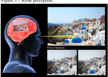
Figure 3 – Scene perception.
Source: Tobii Technology AB (2010).
Visual construction of a complete image from successive fixations.
smooth continuous movements, instead, they make successive jerks, collecting information in
each brief pause in between. When we focus on a specific area of an image or scene, we are basically placing the foveal area of our eyes on top of this region so that the brain gets the highest
resolution of it. The para-foveal and peripheral areas will also capture visual data but with less detail, nevertheless this gives our brain enough information to decide where to move our eyes
next. Thus, we move our eyes in a way so that they can efficiently capture pieces of visual data that our brain then puts together in order to create a complete neat image (see Fig. 3).
3.1.1 Eye movement in reading
We have broadly described the main aspects of eye movement, namely the way we obtain visual information through the use of fixations and saccades. Now we are interested in
analyzing specifically the way we acquire information from a text when we read.
A lot of research has focused on this subject over the last decades, and two theories
regarding the issue of eye-movement control during reading were formerly approached in the literature (PERFETTI, Pitt. notes). The first one is the global control theory which states that eye
movements reflect a global rate (fast eye movements) that is adjusted to accommodate the text difficulty level (O’REAGANet al., 1984). The other one is the direct control theory that says
eye movements reflect moment-by-moment cognitive processing demands during reading (JUST; CARPENTER, 1987). More recent research suggests an in-between scenario, in which language
oculomotor system control where the eyes move (REICHLEet al., 1998).
Over the years, several techniques were applied in order to study how we process
information when reading (CLIFTONet al., 2016). An important conclusion that emerged from
these works, is that three properties of a word can be identified as the factors that most strongly
influence the difficulty with which a word is processed: its frequency (RAYNER; DUFFY, 1986), length (JUHASZet al., 2008) and predictability in context (EHRLICH; RAYNER, 1981).
In general, when studying reading, we are interested in measuring location and duration of fixations and saccades. For adult reading, fixation duration typically vary from about
100-800 ms, with the average being approximately 250 ms. Saccades typically range in duration from about 10-20 ms when readers move their eyes from one word to the next, and for large
saccades, such as moving from the end of one line to the beginning of the next line, may be as long as 60-80 ms (RANEYet al., 2014).
3.2 Eye tracking
There are different eye-tracking systems that detect and track the movements of the eyes and one of the most accurate, non-intrusive techniques is Pupil Centre Corneal Reflection
(PCCR) (GHAOUI, 2005; RANEYet al., 2014). These type of eye trackers basically consist
of a desktop computer with an infrared camera mounted beneath a display monitor, and image
processing software to analyze eye movement data. While the stimuli is presented to the subject on the display monitor, near infrared light from a LED embedded in the camera is shined onto the
subjects’ eyes and the reflections are recorded with the camera. Part of the light is reflected in the cornea, appearing as a small, sharp glint (this is known as the “first Purkinje image"). Another
part reaches the retina and reflects back making the pupil appear as a bright, well defined disc (this is known as the “bright pupil" effect) (see Fig. 4). The reflected images captured by the
camera are then processed so that the center of the pupil and the corneal reflections’ locations are registered. The vector between these two spots is then measured and with further trigonometric
calculations, gaze location is found.
3.2.1 Eye tracking in reading: experimental setup
For the design of our experiment different types of texts were selected, in order
Figure 4 – Corneal reflection and bright pupil effect.
Source: ).
Tobii Eye Tracking. An introduction to eye tracking and Tobii Eye Trackers.
complexity and structure of the text. We include a children story, a scientific text, various excerpts
from literature work, and one random word generated text (RANDOM TEXT GENERATOR, website) that actually makes no sense, all texts in Portuguese, namely:
“Conto Esmeralda" , a story for children, a random generated text,
an excerpt from “Jubiabá" of Jorge Amado (1935, Brazil), an excerpt from “O gaúcho" of José de Alencar (1870, Brazil),
an excerpt from “História do Cerco de Lisboa" of José Saramago (1989, Portugal), an excerpt from “A mão e a Luva" of Machado de Assis (1874, Brazil),
an excerpt from a Wikipedia entrance on the photoelectric effect.
Each text is edited so that the font is mono-spaced with a size of 12 points (see Fig. 22 and Appendix C). For our equipment setup, these characteristics verify that a visual angle of
1◦spans a length of 3 characters, which gives us word position accuracy (RANEYet al., 2014).
The test described here was conducted using an SR Research EyeLink 1000 eye
tracker, with Desktop Mount Participant Setup, Monocular (SR Research Ltd), which operates as described in the previous section. To run the experiment, the subject seats in front of the
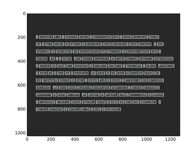
Figure 5 – Example of displayed text.
❖ ❝♦r❛çã♦✱ ❢ê✲❧♦ ❛ ♥❛t✉r❡③❛ ❢r❛♥❝♦ ❡ ❞❡s❝♦rt✐♥❛❞♦ ❝♦♠♦ ❛ ✈❛st❛ ❝♦①✐❧❤❛❀ ❛ ♣❛✐①ã♦
q✉❡ ♦ ❛❣✐t❛ ❧❡♠❜r❛ ♦s í♠♣❡t♦s ❞♦ ❢✉r❛❝ã♦❀ ♦ ♠❡s♠♦ ❜r❛♠✐❞♦✱ ❛ ♠❡s♠❛ ♣✉❥❛♥ç❛✳ ❆ ❡ss❡
t✉r❜✐❧❤ã♦ ❞♦ s❡♥t✐♠❡♥t♦ ❡r❛ ✐♥❞✐s♣❡♥sá✈❡❧ ✉♠❛ ❛♠♣❧✐t✉❞❡ ❞❡ ❝♦r❛çã♦✱ ✐♠❡♥s❛ ❝♦♠♦ ❛
s❛✈❛♥❛✳ ❚❛❧ é ♦ ♣❛♠♣❛✳ ❊st❛ ♣❛❧❛✈r❛ ♦r✐❣✐♥ár✐❛ ❞❛ ❧í♥❣✉❛ q✉í❝❤✉❛ s✐❣♥✐❢✐❝❛ s✐♠♣❧❡s♠❡♥t❡
♦ ♣❧❛✐♥♦❀ ♠❛s s♦❜ ❛ ❢r✐❛ ❡①♣r❡ssã♦ ❞♦ ✈♦❝á❜✉❧♦ ❡stá ✈✐✈❛ ❡ ♣❛❧♣✐t❛♥t❡ ❛ ✐❞❡✐❛✳ Pr♦♥✉♥❝✐❛✐
♦ ♥♦♠❡✱ ❝♦♠ ♦ ♣♦✈♦ q✉❡ ♦ ✐♥✈❡♥t♦✉✳ ◆ã♦ ✈❡❞❡s ♥♦ s♦♠ ❝❤❡✐♦ ❞❛ ✈♦③✱ q✉❡ r❡❜♦❛ ❡ s❡
✈❛✐ ♣r♦♣❛❣❛♥❞♦ ❡①♣✐r❛r ♥♦ ✈❛❣♦✱ ❛ ✐♠❛❣❡♠ ❢✐❡❧ ❞❛ s❛✈❛♥❛ ❛ ❞✐❧❛t❛r✲s❡ ♣♦r ❤♦r✐③♦♥t❡s
✐♥❢✐♥❞♦s❄ ◆ã♦ ♦✉✈✐s ♥❡ss❛ ♠❛❥❡st♦s❛ ♦♥♦♠❛t♦♣❡✐❛ r❡♣❡r❝✉t✐r ❛ s✉r❞✐♥❛ ♣r♦❢✉♥❞❛ ❡
♠❡r❡♥❝ór✐❛ ❞❛ ✈❛st❛ s♦❧✐❞ã♦❄ ◆❛s ♠❛r❣❡♥s ❞♦ ❯r✉❣✉❛✐✱ ♦♥❞❡ ❛ ❝✐✈✐❧✐③❛çã♦ ❥á ❜❛❜✉❥♦✉
❛ ✈✐r❣✐♥❞❛❞❡ ♣r✐♠✐t✐✈❛ ❞❡ss❛s r❡❣✐õ❡s✱ ♣❡r❞❡✉ ♦ ♣❛♠♣❛ s❡✉ ❜❡❧♦ ♥♦♠❡ ❛♠❡r✐❝❛♥♦✳ ❖
❣❛ú❝❤♦✱ ❤❛❜✐t❛♥t❡ ❞❛ s❛✈❛♥❛✱ ❞á✲❧❤❡ ♦ ♥♦♠❡ ❞❡ ❝❛♠♣❛♥❤❛✳
Source: Elaborated by the author, from the novel “O gaúcho" of the Brazilian author José de Alencar.
at a set of dots on the screen, located at known positions, so that the eye tracker measures eye variables for each point (corneal and pupil reflections). Through a validation process, we check
accuracy of the system, that is, how well the calculated fixation locations match new fixations on the same points. We make sure not to surpass a 0.25◦−1◦error. Before starting the experiment,
participants are told that they will be asked a simple question after reading each text. We do this in order to ensure that the participant will commit to consciously read the text. Texts are shown
on the display screen so that the subject can read one by one. To ensure the reading follows as naturally as possible, we do not impose a time limit. While the experiment is running and
the subject reading, the eye tracker collects gaze location at a sample rate of 1000 Hz. This means the eye position is measured every 1 ms, which gives an average temporal error of 0.5 ms
(approximately half the duration of the time between samples) (RANEYet al., 2014).
A group of twenty people was analyzed. This group is homogeneous, primarily
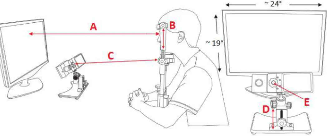
Figure 6 – Experimental setup.
Source: SR RESEARCH SUPPORT FORUMS (website).
A) Eye-to-monitor distance of approximately 80.0 cm, which gives screen dis-play angles of 24◦horizontally and 19◦vertically. This ensures that the display
image falls within the trackable range. B) Participants’s eyes aligned with the top quarter of the monitor. C) Participant to tracker distance of approximately 53.0 cm. D) and E) Eye tracker positioned below the monitor and centered.
3.3 Maximum entropy model applied to fixation configurations
We begin the description of the data analysis method by explaining how fixation
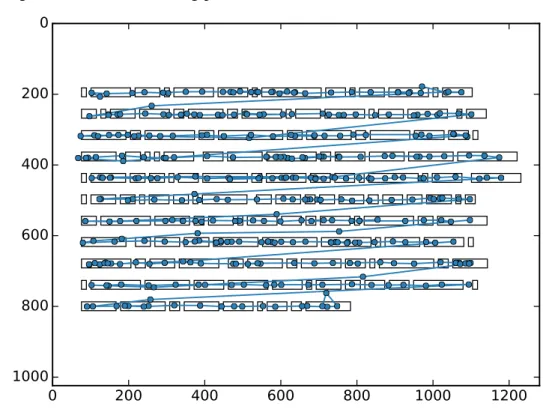
series are constructed. For each text, we define the space coordinates for the words by delimiting each word with a rectangle or “box" (see Fig. 7). This way we are able to link the fixation
coordinates data obtained from the eye tracker to these boxes, and we can count how many fixations fall into each box (word). Then, for each subjecti, we build a sequence of the full text
so that each wordris assigned a stateσr
i =±1, depending on the number of fixationsnrf ix the subject had on the word, according to the following rule,
σir=
+1 ifnrf ix≥2
−1 ifnrf ix<2 . (3.1)
Here, we choose a threshold ofnf ix=2 for the number of fixations that define the active state. This criterion is based on the fact that people look at essentially every word when reading a text (CLIFTONet al., 2016), so in order to differentiate two fixation sequences, we should at least
consider words that are looked at more than one time.
Once we have the fixation series, we calculate the pairwise correlations of fixations
for every pair of subjectsiand jalong themwords of the text,
Figure 7 – Example of text with words delimited by boxes.
0 200 400 600 800 1000 1200
0
200
400
600
800
1000
Source: Elaborated by the author, from the novel “O gaúcho" of the Brazilian author José de Alencar.
where,
hσii= 1
m
m
∑
r=1
σir (3.3)
and
hσiσji= 1
m
m
∑
r=1
σirσrj. (3.4)
Next, we wish to use the minimal statistical model that describes the relations
between subjects’ fixation patterns across the group of people. The probability distribution for this model must maximize the entropy while reproducing the mean value of fixationshσiiand correlations Ci j for all subjects. This is basically the maximum entropy model described in Chapter 2. Let us denoteσ ={σ1r, ...,σNr}the state of the system of theNsubjects when fixating
the wordr. Given that each subject can be in one of two states (+1 or−1), overall we have a set
{σ}of 2N possible states the system can be in, for each word in the text. Following the steps
First, we demand pto be normalized,
∑
{σ}
p({σ}) =1. (3.5)
We also impose that the first moment of variableσimatches the sample mean, fori=1, ...,N,
hσiip=
∑
{σ}
p({σ})σi=hσii= 1
m
m
∑
r=1
σir, (3.6)
and the second moment of variables σi and σj equals the measured correlation values, for
i,j=1, ...,N,i6= j,
hσiσjip=
∑
{σ}
p({σ})σiσj=hσiσji= 1
m
m
∑
r=1
σirσrj. (3.7)
Finally, p({σ})must maximize the entropy,
S=−
∑
{σ}p({σ})ln p({σ}). (3.8)
Then, the Lagrangian associated to Eqs. (3.5-3.8) is of the form,
L =S+λ0(h1ip−1) + N
∑
i=1
λ1i(hσiip− hσii) +
N
∑
i,j=1
λ2i j(hσiσjip− hσiσji), (3.9)
and we need to solve,
∂L
∂p({σ}) =0 ⇒ −lnp({σ})−1+λ0+
N
∑
i=1
λ1iσi+
N
∑
i,j=1
λ2i jσiσj=0, (3.10)
whereλ0, {λ1i} and {λ2i,j} are the Lagrange multipliers. The solution for Eq. (3.10) is the
pairwise maximum-entropy probability distribution,
p({σ}) = 1 Zexp
N
∑
i=1
λ1iσi−
N
∑
i,j=1
λ2i jσiσj
, (3.11)
whereZis the partition function that represents the normalization constant,
Z=
∑
{σ}exp
N
∑
i=1
λ1iσi+ N
∑
i,j=1
λ2i jσiσj
=exp(1−λ0). (3.12)
We note that the expression of Eq. (3.11) is equal to Boltzmann’s probability distribution at
temperatureT =1, where the exponent represents the Hamiltonian,
pT = 1
Ze −E/T
Moreover, for the pairwise maximum-entropy model the energy term is of the same form as that of the Ising model1, withλ
1i =hiandλ2i j =Ji j,
E =−
N
∑
i=1 hiσi−
N
∑
i,j=1
Ji jσiσj. (3.14)
This correspondence motivates us to interpret parametershias the action of the external stimulus (text) acting on subjecti, andJi j as “interactions" between subjectsiand j, although subjects never really interact with each other. In this sense, we can think of the text as a medium through
whichσi couples withσj. It is worth noting that the fact that we can represent the system of fixation configurations by means of the Ising model is due to the binary-state description we
proposed and the choice of measuring mean values and pairwise correlations we made; other choices would result in different models.
Following the method described in Appendix B, we seek the fields hi and the interactionsJi j that reproduce the experimental “magnetizations"hσiiand correlationsCi j, while maximizing the entropy of the system. Once we compute the values ofhiandJi j for all subjects, we are able to write the probability distribution of Eq. (3.13) for our system.
Continuing with the interpretation of our system as a group of interacting subjects, we consider the Boltzmann distribution, where the temperatureT captures the level of fluctuations
of states{σ}along the text. So we set the “operating temperature"To, that is, the temperature when the subjects are reading the text, equal to 1. Then, once we have the probability distribution
that characterizes the system (atT =To=1), we are able to see how the average energy of the system changes for different values ofT. This rate of change is equal to the heat capacity, that is,
how much energy the system can absorb as the temperatureT increases,
Cv=
∂hEipT
∂T . (3.15)
At a critical temperatureTc,Cvis maximal (diverges in the thermodynamic limit), which could be indicative of a phase transition. Then, ifTc<To=1, the system would be in a “liquid" or random state, and as the system becomes more ordered,TcapproachesTo=1.
1 Essentially, the Ising model represents a system ofNinteracting spins arranged in a lattice, where the spins can
4 RESULTS
In this chapter we present and discuss the results obtained from the experiment described in Section 3.2.1 and analyze the data with the model described in Section 3.3. We
first show an example of data collecting for “O gaúcho" text, to have a better image of how an experiment outcome looks like and how the data are organized. In Fig. 8 we show one subject’s
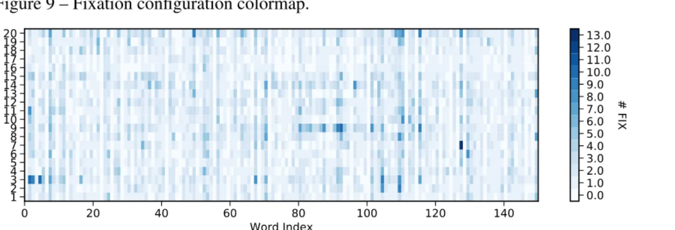
fixation reading pattern, and in Fig. 9 we plot a colormap of the fixation sequences for the complete group. These fixation arrays will be the base for the analysis.
Figure 8 – Fixation reading pattern.
0 200 400 600 800 1000 1200
0
200
400
600
800
1000
Source: Elaborated by the author.
Fixation data registered from participant # 20’s eye tracking, for José de Alen-car text, “O gaúcho". The lines connecting the dots (fixations) represent the movement direction of the eye between fixations but do not correspond to the saccades exactly.
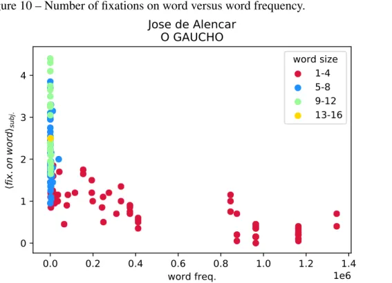
In order to study the relation between the number of fixations and the size and frequency of a word, we generate a database of word size (number of letters in the word) and
word frequency (see Appendix A) for all words in every text. In Fig. 10 we plot the subjects’ average number of fixations on each word as a function of the word frequency. In addition, we
divide the data into groups of different word sizes. We can clearly see that the average number of fixations decreases both with the frequency and the size of the word. This result is reasonable
Figure 9 – Fixation configuration colormap.
0 20 40 60 80 100 120 140
Word Index 1 2 3 4 5 6 7 8 9 10 11 12 13 14 15 16 17 18 19 20 0.0 1.0 2.0 3.0 4.0 5.0 6.0 7.0 8.0 9.0 10.0 11.0 12.0 13.0 # FIX
Source: Elaborated by the author.
Colormap of fixation data obtained from the complete group of participants for José de Alencar text, “O gaúcho".
plot in logarithmic scale, and compare the results for “O gaúcho" and random generated texts. We see that the behaviour is approximately linear, but more disperse for the random text. We
also notice that the average number of fixations is larger for the latter. These differences can also be seen between the random text and the rest of the texts, and we hypothesize that it might be an
indicator of lack of predictability; when a subject encounters unpredictable words while reading, he might need to re-fixate these words trying to find meaning to the text, independently of the
word’s size and frequency.
With the fixation configurations represented in Fig. 9, we determine the states arrays,
following the rule explained in Section 3.3, namely,σr
i = +1 if the number of fixations of subject
iwhen reading wordris≥2 (active),σir=−1 if the number of fixations is<2 (inactive). The
correspondent arrays for “O gaúcho" text are represented in Fig. 12 as a binary colormap. From these arrays we are able to calculate the experimental “magnetizations"hσiiand correlations
Ci j, in order to solve the inverse problem explained in Appendix B. Once we have the estimated values of fieldshiand interactionsJi j, we can write the corresponding Hamiltonian and thus the probability distribution. This allows us to calculate and plot the specific heat as a function of temperature, as we show in Fig. 13. We see that the specific heat curves have a maximum at
a critical temperatureTc, which suggests the existence of a phase transition atT =Tc. Now, at the operating temperatureT =1, that is, the temperature at which the texts are being read, we
see whether the system is above, below or near criticality. Clearly, all texts reading are below criticality, and all, except the random generated one, are near the critical point. From statistical
Figure 10 – Number of fixations on word versus word frequency.
0.0 0.2 0.4 0.6 0.8 1.0 1.2 1.4 word freq. 1e6 0 1 2 3 4 fix .o n w or dsu bj .
Jose de Alencar O GAUCHO word size 1-4 5-8 9-12 13-16
Source: Elaborated by the author.
Subjects average number of fixations on each word as a function of the word frequency, for José de Alencar text, “O gaúcho". Data points are divided into groups of different word sizes (number of letters).
Figure 11 – Number of fixations on word versus word frequency in semi-logarithmic scale.
103 104 105 106
word freq. 0.0 0.5 1.0 1.5 2.0 2.5 3.0 3.5 4.0 4.5 5.0 fix .o n w ord su bj .
Jose de Alencar O GAUCHO word size 1-4 5-8 9-12 13-16
103 104 105 106
word freq. 0.0 0.5 1.0 1.5 2.0 2.5 3.0 3.5 4.0 4.5 5.0 fix .o n w ord su bj . RANDOM TEXT word size 1-4 5-8 9-12 13-16
Source: Elaborated by the author.
Subjects average number of fixations on each word as a function of the word frequency (in logarithmic scale) for José de Alencar text, “O gaúcho" (left) and random text (right). Data points are divided into groups of different word sizes (number of letters).
crystal state). On the other hand, when interactions are too weak, particles behave randomly and
the system becomes “fluid". At some intermediate point, forT =Tc, the correlations between particles are maximal. Thus, this result may suggest that meaningful well written texts highly
correlate the fixation patterns of the subjects’ reading.
Figure 12 – Fixation configuration binary colormap.
0 20 40 60 80 100 120 140
Word Index 1 2 3 4 5 6 7 8 9 10 11 12 13 14 15 16 17 18 19 20 -1 1 Active - Inactive
Source: Elaborated by the author.
Binary colormap of fixation data obtained from the complete group of participants for José de Alencar text, “O gaúcho".
correlation for all pair of subjects,
Ci j = 1
N(N−1)
N
∑
i=1
∑
j6=iCi j. (4.1)
In Table 1 we show the values of critical temperature and average correlation for all texts. We see
that all texts have similar average correlation (although it is noticeable that “Conto Esmeralda" text has a lower value), and there is no clear relation betweenCi j andTc. The absence of such a dependency relation is something we did not expect, although we suppose that the number of texts utilized (the number of experimental points) is possibly not sufficient to detect an evident
behaviour betweenCi j andTc.
Table 1 –Tc,Ci j andhσiifor all texts.
Text Tc Ci j hσii
Conto Esmeralda 0.85 0.1411 -0.5190
Random Text 0.70 0.2678 -0.0464
Jubiaba 0.83 0.2494 -0.3697
O gaúcho 0.83 0.3613 -0.2147
História do Cerco de Lisboa 0.81 0.2758 -0.2918
A mão e a Luva 0.79 0.2878 -0.2460
Efeito fotoelétrico 0.84 0.2411 -0.3984 Source: Elaborated by the author.
Note: Values of critic temperature, average correlation and average “magnetization" for all texts.
In order to get more insight on the different reading patterns and how they relate to
Figure 13 – Specific heat curves obtained for the system of fixation configurations of all texts.
0.00
0.25
0.50
0.75
1.00
1.25
1.50
1.75
2.00
T
0.0
0.2
0.4
0.6
0.8
Cv
Jorge Amado JUBIABA
Wikipedia EFEITO FOTOELETRICO
Machado de Assis A MAO E A LUVA
CONTO ESMERALDA
Jose Saramago HISTORIA DO CERCO DE LISBOA
Jose de Alencar O GAUCHO
RANDOM TEXT
Source: Elaborated by the author.Specific heat curves for all texts. The curves suggest a phase transition atT =Tc. The operating temperatureT =1 is close toTcfor all texts except for the random generated text which has no meaning.
once on each word more than they fixate twice or more times), with the exception of the random
text. In this case, half of the subjects have negativehσiiwhile the other half has positivehσii. This result is interesting and once again shows a distinct difference between meaningful texts
Figure 14 – Mean magnetization for all subjects.
16 17 1 19 10 2 5 6 7 18 11 13 4 15 3 8 12 14 20 9 i (subjects) 0.8 0.7 0.6 0.5 0.4 0.3 0.2 0.1 0.0 0.1 0.2 0.3 0.4 0.5 i
Jose de Alencar O GAUCHO
16 7 1 5 10 17 12 18 13 19 6 15 2 11 14 8 4 9 3 20 i (subjects) 0.8 0.7 0.6 0.5 0.4 0.3 0.2 0.1 0.0 0.1 0.2 0.3 0.4 0.5 i Jose Saramago HISTORIA DO CERCO DE LISBOA
17 5 1 12 14 6 7 16 10 15 18 13 19 9 2 4 11 8 20 3 i (subjects) 0.8 0.7 0.6 0.5 0.4 0.3 0.2 0.1 0.0 0.1 0.2 0.3 0.4 0.5 i CONTO ESMERALDA
17 1 16 5 7 10 6 13 2 8 18 15 4 14 9 11 12 19 20 3 i (subjects) 0.8 0.7 0.6 0.5 0.4 0.3 0.2 0.1 0.0 0.1 0.2 0.3 0.4 0.5 i RANDOM TEXT
16 6 5 1 10 7 12 14 2 17 11 18 13 4 15 19 8 9 3 20 i (subjects) 0.8 0.7 0.6 0.5 0.4 0.3 0.2 0.1 0.0 0.1 0.2 0.3 0.4 0.5 i Jorge Amado JUBIABA
16 1 17 10 4 5 6 7 9 11 12 19 15 18 8 13 14 2 3 20 i (subjects) 0.8 0.7 0.6 0.5 0.4 0.3 0.2 0.1 0.0 0.1 0.2 0.3 0.4 0.5 i
Machado de Assis A MAO E A LUVA
5 8 16 1 7 14 17 18 10 6 12 4 13 3 15 19 11 20 9 2 i (subjects) 0.8 0.7 0.6 0.5 0.4 0.3 0.2 0.1 0.0 0.1 0.2 0.3 0.4 0.5 i Wikipedia EFEITO FOTOELETRICO
Mean magnetizationhσiiof all subjectsi=1, ...,20 for all seven texts.
In Table 1 we also show the subjects’ average magnetizationhσiifor all texts,
hσii= 1
N
N
∑
i=1h
Given the distinct pattern of magnetizations for the random text, we see thathσiifor this text is much closer to zero, in comparison with the other texts. Another thing we notice is that the
“Conto Esmeralda" text has a greater magnetization than the rest of the texts. This means that, in average, the subjects need not to fixate the words more than once, which again can be indicative
of word predictability; we recall that this is a children story and thus it’s literary content is elementary.
In Fig. 15 we plot the critical temperatureTc of all texts as a function of the average magnetizationhσii. We find thatTcincreases linearly withhσii, which makes sense given that the more randomized the magnetizations, the farther from the critical point the system is.
Figure 15 –Tcversus. hσii.
0.6 0.5 0.4 0.3 0.2 0.1 0.0 0.1 i
0.700 0.725 0.750 0.775 0.800 0.825 0.850 0.875 0.900
T
cCONTO ESMERALDA
RANDOM JUBIABA O GAUCHO
HISTORIA DO CERCO DE LISBOA
A MAO E A LUVA EFEITO FOTOELETRICO
Source: Elaborated by the author.
Critical temperatureTcas a function of average magnetizationhσii. The line represents the linear approximation.
In Table 2 we show the values of average interactionsJi j next to the values ofTc,
Ji j = 1
N(N−1)
N
∑
i=1
∑
j6=iJi j. (4.3)
Table 2 –Tc,Ji j andhifor all texts.
Text Tc Ji j hi
Conto Esmeralda 0.46 0.0680 -0.1550
Random Text 0.29 0.0768 -0.0376
Jubiaba 0.15 0.0739 -0.1169
O gaúcho 0.33 0.0793 -0.0452
História do Cerco de Lisboa 0.46 0.0777 -0.091
A mão e a Luva 0.32 0.0771 -0.0637
Efeito fotoelétrico 0.40 0.0754 -0.0910 Source: Elaborated by the author.
Note: Values of critic temperature, average inter-actions and average fields for all texts.
Figure 16 –Ci j vs. Ji j.
0.065 0.070 0.075 0.080 0.085 0.090
J
ij0.10 0.15 0.20 0.25 0.30 0.35 0.40
C
ijCONTO ESMERALDA_Tc= 0.85
RANDOM_Tc= 0.7
JUBIABA_Tc= 0.83
O GAUCHO_Tc= 0.83
HISTORIA DO CERCO DE LISBOA_Tc= 0.81
A MAO E A LUVA_Tc= 0.79
EFEITO FOTOELETRICO_Tc= 0.84
Source: Elaborated by the author.
Average pairwise-correlation as a function of average interactions. These quantities are linearly related.
4.1 Randomizations of fixation configurations
To test that our results are not found for just any random data, we perform a random-ization of the fixation configurations of all subjects for every text, and compare with the original
results. This means that the mean magnetizationshσiifori=1, ...,Nwill remain the same, but strong correlationsCi j should dissapear. Once we have shuffled the data, we follow the same cal-culations as before, namely, we find the pairwise correlationsCi j and mean magnetizationshσii, compute the couplingsJi j and fieldshi, and find the specific heatCvat different temperaturesT. In Fig. 17 we plot the curves of specific heatCvas a function of temperatureT. There is still a maximum inCvfor a critical temperatureTcbut now the texts operating temperatures
To=1 are far fromTc (To≫Tc), for all texts.
In Table 3 we show the resulting values ofTc,Ci j andhσiiafter data shuffling. We see that both the values ofTcandCi j are much lower than the values for the original data. The absence of strong correlations is analogous to state that the system becomes "fluid", being far
Figure 17 – Specific heat curves obtained for the system of fixation configurations of all texts by shuffling the data.
0.00 0.25 0.50 0.75 1.00 1.25 1.50 1.75 2.00
T
0.05
0.10
0.15
0.20
0.25
0.30
0.35
Cv
Jorge Amado JUBIABA
Wikipedia EFEITO FOTOELETRICO
Machado de Assis A MAO E A LUVA
CONTO ESMERALDA
Jose Saramago HISTORIA DO CERCO DE LISBOA
Jose de Alencar O GAUCHO
RANDOM TEXT
Source: Elaborated by the author.Specific heat curves for all texts after shuffling the fixation configurations. The curves exhibit a maximum atT =Tc. The operating temperatureTo=1 is far fromTc for all texts.
reading fixation configurations. Finally, as also shown in Table 3, the effect of shuffling the data
Table 3 –Tc,Ci j,hσii,Ji j andhifor all texts with shuffled data.
Text Tc Ci j hσii Ji j hi
Conto Esmeralda 0.46 -0.0042 -0.5190 -0.0020 -0.7449
Random Text 0.29 -0.0007 -0.0464 0.0021 -0.0767
Jubiaba 0.15 -0.0013 -0.3697 0.0028 -0.4510
O gaúcho 0.33 0.0114 -0.2147 0.0124 -0.2118
História do Cerco de Lisboa 0.46 -0.0034 -0.2918 0.0009 -0.3792
A mão e a Luva 0.32 0.0069 -0.2460 0.0128 -0.2600
Efeito fotoelétrico 0.40 0.0079 -0.3984 0.0077 -0.5176 Source: Elaborated by the author.
5 CONCLUSIONS
In this work we proposed the maximum-entropy probability model to study the relation between the fixation configurations of different people when reading different texts.
More specifically, we were interested in knowing if some types of texts elicit a correlated reading behaviour among different subjects. Aiming to answer this question we designed a reading
experiment with various texts, and by means of a high precision eye-tracking equipment, we were able to collect accurate fixation data for a group of 20 subjects. Since eye movement is a
reflect of cognitive activity in the brain, we expected that the experimental data could give us insight into the way we process information while we read. In particular, the number of fixations
on each word can be associated with the way our attention is focused while we read and how we process each word.
We confirmed previous observations (RAYNER; DUFFY, 1986; JUHASZ et al.,
2008) that the number of fixations on a word decreases with word size and frequency, although
we noticed that in the particular case of a meaningless text (random generated text) this behaviour is not so clear; the number of fixations is, in average, greater than in the other texts, independently
of the size and frequency of the word. The third variable that affects the number of fixations on a word is the word’s (and overall, text’s) predictability. Although we were not able to specifically
quantify this property, our analysis could provide information on the reading behaviour of the subjects, for texts that range different complexities and meanings. In this sense, we observe that
the average number of fixations is indeed greater for a non-predictable text (such as the random text) than for a simple text (such as the “Conto Esmeralda" text, which is a children story).
We used the maximum entropy inference model to describe the system, which is the minimal statistical model that is in agreement with the given experimental data (correlations
Ci j and “magnetizations"hσii) and does not imply any extra assumptions. For our system, the pairwise maximum-entropy probability distribution takes the form of the Boltzmann distribution
withT =1 for an Ising type configuration, that is, an arrangement ofNelements that can be in
one of two statesσi= +1 orσi=−1, each pairiand jwith an interactionJi j. In our case, for each subjectithe stateσr
i is defined as positive if wordris fixated more than once, and negative if it is fixated once or not fixated at all. As for the interactionsJi j, although the subjects do not actually interact with each other, we can think of the text as a medium through which they can be statistically coupled. Furthermore, considering that the temperatureT of the Boltzmann equation
temperatureTo=1 and study how the energy changes with the temperature (specific heat). In this way, it was possible to analyze the fluctuations in the system, which is representative of the
collective behaviour.
Our results show that, for the system of readers’ fixation configurations, Cv is maximal at a critical temperatureTcand the system is above and near criticality for meaningful texts (Tc∼To=1), whereas for an incoherent text (random generated text) the system seems to be in a much disordered state (Tc<To). This means that, apparently, readers correlate their attention patterns when reading coherent texts, but do not correlate when reading something meaningless.
It is worth noting that this type of global behaviour arises from weak pairwise interactions, which means that the system exhibits emergent properties out of local interactions. This conclusion
is reinforced after performing a randomization of the subjects’ fixation configurations; indeed the system is far from criticality in this case, and correlations diminish drastically. Although we
were not able to find a clear relation between the subjects’ average correlationCi jand the critical temperatureTc, we suspect that the number of texts used in this work may not be sufficient to see a reliable statistical behaviour between both. As for the average “magnetizations", we found that
hσiiincreases with the critical temperatureTc, which makes sense since a more random state is expected to be far away from criticality.
Overall we think the results obtained in this work are interesting and contribute to
the study of the human fixating behaviour while reading, which we consider of great importance given that eye-movement and eye-fixation are directly related to cognitive activity. We were able
to distinguish distinct reading behaviours for some of the texts, in particular a clear coherence between subjects when reading a meaningful text, which weakened significantly for the case
BIBLIOGRAPHY
BURLESON-LESSER, K.; MORONE, F.; DEGUZMAN, P.; PARRA, L. C.; MAKSE, H. A. Collective behaviour in video viewing: A thermodynamic analysis of gaze position. PLOS ONE, Public Library of Science, v. 12, n. 1, p. 1–19, 01 2017.
BURY, T. Statistical pairwise interaction model of stock market.The European Physical Journal B, v. 86, n. 3, p. 89, 03 2013.
CLIFTON, C.; FERREIRA, F.; HENDERSON, J. M.; INHOFF, A. W.; LIVERSEDGE, S. P.; REICHLE, E. D.; SCHOTTER, E. R. Eye movements in reading and information processing: Keith rayner’s 40 year legacy.Journal of Memory and Language, v. 86, p. 1–19, 2016. CORPUS DO PORTUGUÊS. Disponível em: <https://www.corpusdoportugues.org/>.
EHRLICH, S. F.; RAYNER, K. Contextual effects on word perception and eye movements during reading.Journal of Verbal Learning and Verbal Behavior, v. 20, n. 6, p. 641–655, 1981.
ERDÖS, P.; RÉNYI, A. On random graphs i.Publicationes Mathematicae Debrecen, v. 6, p. 290–297, 1959.
EYE ANATOMY. website. Disponível em: <http://spectaclegallery.com/eye-anatomy/>.
GHAOUI, C.Encyclopedia of Human Computer Interaction. [S.l.]: Idea Group Reference, 2005. 211–219 p. (ITPro collection). Chapter: Eye Tracking in HCI and Usability Research. ISBN 9781591407980.
JAYNES, E. T. Information theory and statistical mechanics. Physical Review, American Physical Society, v. 106, p. 620–630, 05 1957.
JAYNES, E. T. Information theory and statistical mechanics. ii.Physical Review, American Physical Society, v. 108, p. 171–190, 10 1957.
JUHASZ, B. J.; WHITE, S. J.; LIVERSEDGE, S. P.; RAYNER, K. Eye movements and the use of parafoveal word length information in reading.Journal of Experimental Psychology: Human Perception and Performance, v. 34, n. 6, p. 1560–1579, 12 2008.
JUST, M. A.; CARPENTER, P. A.The psychology of reading and language comprehension. [S.l.]: Needham Heights, MA, US: Allyn Bacon, 1987. ISBN 0-205-08760-4.
O’REAGAN, J. K.; LEVY-SCHOEN, A.; PYNTE, J.; BRUGAILLERE, B. Convenient fixation location within isolated words of different length and structures. Journal of Experimental Psychology: Human Perception and Performance, v. 10, n. 2, p. 250–257, 4 1984.
PERFETTI, C. A.Eye Movements in Reading. Pitt. notes. University of Pittsburgh, Perfetti notes. Disponível em: <http://www.pitt.edu/~perfetti/EyeMovementsDuringReading.htm>.
RANDOM TEXT GENERATOR. website. Disponível em: <http://randomtextgenerator.com/>.
RAYNER, K.; DUFFY, S. A. Lexical complexity and fixation times in reading: Effects of word frequency, verb complexity, and lexical ambiguity.Memory & Cognition, v. 14, n. 3, p. 191–201, 05 1986.
REICHLE, E.; POLLATSEK, A.; FISHER, D.; RAYNER, K. Toward a model of eye movement control in reading.Psychological Review, v. 105, p. 125–157, 1998.
SHANNON, C. E. A mathematical theory of communication. SIGMOBILE Mob. Comput.
Commun. Rev., v. 5, n. 1, p. 3–55, 01 2001.
SR RESEARCH SUPPORT FORUMS. website. Disponível em: <https://www.sr-support.com/>.
STEIN, R. R.; MARKS, D. S.; SANDER, C. Inferring pairwise interactions from biological data using maximum-entropy probability models.PLOS Computational Biology, v. 11, n. 7, p. 1–22, 07 2015.
TKACIK, G.; SCHNEIDMAN, E.; J., B. M.; W., B. Ising models for networks of real neurons. 2006. Disponível em: <arXiv:q-bio/0611072>.
TOBII TECHNOLOGY AB.An introduction to eye tracking and Tobii Eye Trackers. 2010.
TRIBUS, M.; MCIRVINE, E. C. Energy and information. Scientific American, Scientific American, a division of Nature America, Inc., v. 225, n. 3, p. 179–190, 1971.
WADE, N. J. Pioneers of eye movement research.i-Perception, v. 1, n. 2, p. 33–68, 2010. WU, X. Calculation of maximum entropy densities with application to income distribution.
APPENDIX A – WORD FREQUENCY REGISTER
In linguistics, a text corpus is a large and structured set of texts (usually electronically stored and processed), that are used to do statistical analysis and hypothesis testing, checking
occurrences or validating linguistic rules within a specific language environment. Texts used in this work are part of the Portuguese language corpus “O Corpus do português" database
(CORPUS DO PORTUGUÊS, ). This corpus contains 45 million words dating from centuries XIII to XX, and for the XX century it is equally divided between spoken, fiction, newspaper, and
academic texts.
The texts we selected specifically date from centuries XIX and XX, so we used a
sub-corpus of the texts from this period to collect word occurrence data. For each of our texts, we search every word in the corpus and register it’s number of occurrences in the sub-corpus. In
Fig. 18 we plot an histogram that shows the distribution of the percentage of words in the text with a certain number of occurrences in the sub-corpus. The number of occurrences ranges from
0 to 1.4 106and is divided in 200 bins. We can see that, for the “O gaúcho" text, the percentage of words with rare occurrences is much larger than for the “Conto Esmeralda" text, which makes
sense given that the latter is a children story and thus uses simpler (more frequent) words.
Figure 18 – Corpus word occurrence histogram.
0.0 0.2 0.4 0.6 0.8 1.0 1.2 1.4 Corpus occurrence 1e6 0.00
0.05 0.10 0.15 0.20 0.25 0.30 0.35 0.40 0.45 0.50 0.55
Number of words (percentage)
Jose de Alencar O GAUCHO
0.0 0.2 0.4 0.6 0.8 1.0 1.2 1.4 Corpus occurrence 1e6 0.00
0.05 0.10 0.15 0.20 0.25 0.30 0.35 0.40 0.45 0.50 0.55
Number of words (percentage)
CONTO ESMERALDA
Source: Elaborated by the author.
APPENDIX B – METROPOLIS ALGORITHM
We consider a network with couplings determined by the Erdös and Rényi graph model (ERDÖS; RÉNYI, 1959). We get a setG(N;p)of random graphs by building networks of
N vertices, where the probability of connection is given by,
p= k
N−1, (B.1)
where k is the mean connectivity between two vertices. For k=0 none of the vertices are connected, and for k=N−1 the network is fully connected (if all edges are created). Once
we know which elements are connected, we can attribute random values of couplings{Ji j}and fields{hi}(withJi j =0 for elementsσi σj that are not connected). Couplings are distributed according to a Gaussian with mean valueµ and standard deviationσ (do not mistake with theσ
notation used to represent the state of the system),
P(Ji j) = 1
σ√2πexp
" −12
Ji j−µ
σ
2#
(B.2)
In this work, we use µ =0, standard deviationσ =0.25 andJi j∈[−1,1]. The fields{hi}are uniformly distributed in an interval[0,1].
For the Metropolis algorithm, a new state is generated by the following procedure;
we have a stateσµ ={σ1µ, ...,σNµ}(whereNis the number of subjects), of energyEµ (given by
Eq. (3.14)). At each step, we randomly change one of theσiand calculate for the new system
σν the energyEν. The new state can be accepted or rejected with probability,
P=
e−β(Eν−Eµ) ifE
ν−Eµ>0
1 ifEν−Eµ≤0
. (B.3)
This way, if the new state has a lower energy than the previous one, the state is accepted; on the contrary, if the new state has a greater energy than the previous state, the state is accepted with
probability given by Eq. (B.3). Each of these steps determines a Monte Carlo step. Following this algorithm we generate a set of states, at a certain temperature, and we can calculate the
mean values we need. From the initial state, we performτeqMonte Carlo steps until the system reaches equilibrium, and thenτMCsteps until we obtain our set of states. In order to produce less
correlated states, we use states generated every 2N steps. Then, to obtainmindependent states
and then update the couplingsJi j andhiaccording to the rules,
Ji j(t+1) =Ji j(t) +∆Ji j(t+1)
∆Ji j(t+1) =ε
hσiσji − hσiσjith
(t)
(B.4)
and,
hi(t+1) =hi(t) +∆hi(t+1)
∆hi(t+1) =ε[hσii − hσiith] (t)
. (B.5)
wheret is the index of each run and the parameterε is set to 0.1. Here,hσiiandhσiσjiare the experimental mean values. For every update, we calculate the mean values and measure the
distance between the present update and the former so that,
∆hσi(t) = 1 N
N
∑
i=1
(hσii(t)−(hσii(t−1))2 (B.6)
and,
∆hσ σi(t) = 2
N(N−1)i
∑
<j(hσiσji(t)−(hσiσji(t−1))2. (B.7)