The relationship between 0.25–2.5 μm aerosol and CO<sub>2</sub> emissions over a city

(1)

ACPD

10, 21521–21545, 2010

The relationship between 0.25–2.5 µm

aerosol and CO₂ emissions

M. Vogt et al.

Title Page

Abstract Introduction

Conclusions References

Tables Figures

◭ ◮

Back Close

Full Screen / Esc

Printer-friendly Version

Interactive Discussion

Discussion

P

a

per

|

Dis

cussion

P

a

per

|

Discussion

P

a

per

|

Discussio

n

P

a

per

Atmos. Chem. Phys. Discuss., 10, 21521–21545, 2010 www.atmos-chem-phys-discuss.net/10/21521/2010/ doi:10.5194/acpd-10-21521-2010

Atmospheric Chemistry and Physics Discussions

This discussion paper is/has been under review for the journal Atmospheric Chemistry and Physics (ACP). Please refer to the corresponding final paper in ACP if available.

The relationship between 0.25–2.5 µm

aerosol and CO

₂

emissions over a city

M. Vogt1, E. D. Nilsson1, L. Ahlm1, E. M. M ˚artensson1, and C. Johansson1,2

1

Department of Applied Environmental Science (ITM), Stockholm University, 10691 Stockholm, Sweden

2

City of Stockholm Environment and Health Administration, Box 8136, 10420 Stockholm, Sweden

Received: 19 July 2010 – Accepted: 12 August 2010 – Published: 9 September 2010 Correspondence to: M. Vogt (matthias.vogt@itm.su.se)

(2)

ACPD

10, 21521–21545, 2010

M. Vogt et al.

Title Page

Tables Figures

◭ ◮

Back Close

Full Screen / Esc

Discussion

P

a

per

|

Dis

cussion

P

a

per

|

Discussion

P

a

per

|

Discussio

n

P

a

per

|

Abstract

Unlike exhaust emissions, non-exhaust tra_ffic emissions are completely unregulated and there are large uncertainties in the non-exhaust emission factors required to esti-mate the emissions of these aerosols. This study provides the first published results of direct measurements of size resolved emission factors for particles in the size range

5

0.25–2.5 µm using a new approach deriving aerosol emission factors from the CO₂ emission fluxes. Because the aerosol and CO₂emissions have a common source and because the CO₂emission per fuel or tra_ffic amount are much less uncertain than the aerosol emissions, this approach has obvious advantages. Therefore aerosol fluxes were measured during one year using the eddy covariance method at the top of a

10

118 m high communication tower over Stockholm, Sweden. Maximum CO₂ and parti-cle fluxes coincides with the wind direction with densest tra_ffic within the footprint area. Negative fluxes (uptake of CO₂ and deposition of particles) coincides with an urban forest area. The fluxes of CO₂ were used to obtain emission factors for particles by assuming that the CO₂fluxes could converted to amounts of fuel burnt. The estimated

15

emission factors for the fleet mix in the measurement area are, in number 1.4×1011

[particle veh−1_km−1_{]. Assuming spherical particles of density 1600 kg/m}3 _this

corre-sponds to 27.5 mg veh−1_km−1_{. Wind speed influence the emission factor indicating}

that wind induced turbulence may be important.

1 Introduction

20

Road tra_ffic is one of the major contributors to air pollution in many urban areas (Ru-uskanen et al., 2001; Gidhagen et al., 2005). Airborne particulate matter (PM) may be expressed in terms of number mass, surface area, or volume (Harrisson et al., 2000), but PM₁₀ and PM_2.5 are the usual metrics used in regulations of air pollution within Europe. This despite the fact that information about bulk particle mass concentrations

25

(3)

ACPD

10, 21521–21545, 2010

M. Vogt et al.

Title Page

Tables Figures

◭ ◮

Back Close

Full Screen / Esc

Discussion

P

a

per

|

Dis

cussion

P

a

per

|

Discussion

P

a

per

|

Discussio

n

P

a

per

effects of aerosol pollution. Particle size resolved information on emissions is urgently needed to understand processes controlling emissions and the importance for health and climate. In order to make accurate air quality and tra_ffic measurements, good source apportionment is needed. This in turn means that emission inventories should include relationships between meteorology, tra_ffic intensity, fuel load, etc.

5

A number of studies have been made and approaches used (see below) to quantify road traffic emissions for different applications.

The

– laboratory dynamometer test, which provides emission factors (EFs) for individual vehicles including gasoline/diesel light duty vehicles and heavy duty EFs (see e.g.,

10

Westerholm and Egeback, 1994; Sj ¨ogren et al., 1996; Hall et al., 2001; etc.)

– car-chasing experiments and the FEAT-technique provide EFs for individual vehi-cles in real world driving (Kittelson et al., 2000; Sj ¨odin and Lenner, 1995).

– open-road studies Open-road studies are based on a combination of roadside measurements of air pollutants and models to account for the dispersion of the

15

exhaust gas plume. Information about the evolution of EFs for PM₁₀ and PM₁ (Gehrig et al., 2003) as well as for particle number, active particle surface area, and black carbon (BC) (Jamriska and Morawska, 2001) has been derived using this technique.

– road tunnel measurements which provide EFs from the entire fleet during partly

20

real-world conditions (e.g. McLaren et al., 1996; Kristensson et al., 2004; Colberg et al., 2005; Hueglin et al., 2006).

– eddy covariance method which provides also EFs for entire fleet for actual real world conditions (Dorsey et al., 2002; M ˚artensson et al., 2006; Martin et al., 2008; J ¨arvi et al., 2009). It requires fast response instrumentation.

25

(4)

ACPD

10, 21521–21545, 2010

M. Vogt et al.

Title Page

Tables Figures

◭ ◮

Back Close

Full Screen / Esc

Discussion

P

a

per

|

Dis

cussion

P

a

per

|

Discussion

P

a

per

|

Discussio

n

P

a

per

|

from a large vehicle fleet during real-world driving and under the influence of diff er-ent meteorological conditions that might a_ffect the emissions. On the other hand the obtained emissions fluxes are strongly dependent on wind direction and the footprint of the measurement site. Measuring vertical fluxes allow us to develop accurate and e_fficient parameterizations (Dorsey et al., 2002; M ˚artensson et al., 2006; Martin et al.,

5

2008). Functional relationships between aerosol emissions and CO₂emissions, which both originates from a common source, suggest the possibility of using carbon dioxide (CO₂) flux as a tra_ffic tracer. The amount of CO₂ produced from vehicle combustion and fossil fuel is well known and varies much less than the aerosol (Vogt et al., 2010, Bayerisches Landesamt fuer Umwelt). The later change not only in concentration but

10

also in size and internal external mixing. Measurement results shown below will be used to calculate size resolved EFs in the size range of (Dp, 0.25–2.5 µm).

2 Measurement site and instrumentation

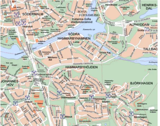
The measurements were made in Stockholm (Sweden), from the top of a telecommu-nication tower in the southern central part of the city. The tower is built in concrete,

15

105 m tall and located 28 m above the sea level. (Latitude North 59◦₁′_0.43′′_and

Lon-gitude: East 18◦₅′_53.17′′_{). On the top of the tower there is an elevator machine room}

and on top of that there is a 11 m high metal frame with a 2.5_×2.5 m platform at the top. This platform enable us to extend the flux measurements far enough from the bulkier concrete construction to avoid flow distortion caused by the tower. Central Stockholm,

20

with high tra_ffic activity, is located north of the tower. A wide forest area dominates in the easterly direction. Significant green sectors can also be found to the east through to the south-west mixed with residential areas.

Because the focus of this study is road tra_ffic aerosol emissions, more details are provided on the larger streets lying in the footprint area of interest. The communication

25

(5)

ACPD

10, 21521–21545, 2010

M. Vogt et al.

Title Page

Tables Figures

◭ ◮

Back Close

Full Screen / Esc

Discussion

P

a

per

|

Dis

cussion

P

a

per

|

Discussion

P

a

per

|

Discussio

n

P

a

per

roads in the neighborhood of the tower, with around 50 000 vehicles per day. S ¨odra L ¨anken, is an underground freeway tunnel with one exit located in the Northeast of communication the tower (see Fig. 1). The site has been previously described by M ˚artensson et al. (2006) and Vogt et al. (2010)

2.1 Instruments and measurement setup

5

The instrumentation consists of a Gill (R3) ultrasonic anemometer, an open path in-frared CO₂/H₂O analyzer LI-COR 7500 (LI-COR, Inc., Lincoln, Nebraska 68504, USA), and two identical Optical Particle Counters (OPC) (Model, 1.109, Grimm Ainring, Bay-ern, Germany) in a housing with a system to heat and dry the sampled air (Grimm Model 265, special version going up to 300◦_{C). The sample air was dried by 1:1}

di-10

lution with 0% humidity particle free air, which minimizes the risk of unwanted loss of semi-volatile compounds, compared to simply heating the air in order to dry it. (Detailed information can be found in Vogt et al., 2010)

2.2 Eddy covariance method, data processing corrections and errors

The vertical aerosol number flux was calculated using the eddy covariance technique

15

(EC). For this study the fluxw′_N_{was calculated over periods of 30 min. The fluctuations} w′ _and _N′ _{were separated from the mean by linear de-trending, which also removes}

the influence of low frequency trends.

The validity of the EC technique at the measurement location was confirmed in ear-lier studies (M ˚artensson et al., 2006; Vogt et al., 2010). The fluxes have been corrected

20

due to the limited time response of the sensor and attenuation of turbulent fluctuations in the sampling line. The response time constantτ_c for both OPC and sampling line was estimated to be 1.5 s by using transfer equations for damping of particle fluctu-ations in laminar flow (Lenschow and Raupach, 1991) and in a sensor (Horst et al., 1997). The typical magnitude of these corrections varied, resulting in an

underestima-25

(6)

ACPD

10, 21521–21545, 2010

M. Vogt et al.

Title Page

Tables Figures

◭ ◮

Back Close

Full Screen / Esc

Discussion

P

a

per

|

Dis

cussion

P

a

per

|

Discussion

P

a

per

|

Discussio

n

P

a

per

|

CO₂has been corrected for variations in air density due to fluctuation in water vapor and heat fluxes in accordance with Webb et al. (1980). This resulted in a maximum increase around noon for CO₂of∼37%.

In addition the aerosol fluxes and concentrations were corrected for tube losses in the sampling line, which resulted in particle losses of_∼5% for the largest size class in

5

the OPC (Dp=2 µm to 2.5 µm).

3 Results

The measurements in this study were performed from 1st of April 2008 to the 15th of April 2009. About 45% of the data has been removed due to instrumental problems, mostly due to rain. An open path infrared CO₂/H₂O analyzer was used which resulted in

10

large spikes in the data set associated with rain events. In addition to the spike removal, half hourly data were rejected when the atmosphere was not turbulent (u_∗<0.1 m s−1₎

and from 12.12.2008 to 21.1.2009 no LICOR data were available.

3.1 Wind direction and sector selection

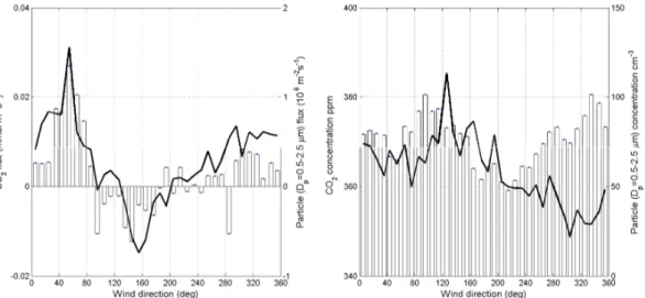
The wind direction dependency of the particle number concentration and flux and the

15

CO₂ flux and concentration is shown in Fig. 2. The data has been sorted into mean values in 10◦ _{bins for the incoming wind direction. The CO}

2 and particle fluxes show similar wind direction dependencies. The highest values for the CO₂ and particle flux are found to the Northeast (40 to 80◦_{). This maximum coincides with the densest}

tra_ffic within the footprint area. A minimum in the fluxes is found in the East to South

20

(90 to 180◦_{). The CO}

2 flux shows negative values within this sector indicating that the photosynthetic activity from the urban forest located in the East dominates surface carbon exchange in this area. The particle fluxes also show negative values (120 to 200◦_{) indicating that deposition of particles is the most important particle surface}

exchange process in this wind sector. Particle fluxes as well as CO₂ fluxes increase

25

(7)

ACPD

10, 21521–21545, 2010

M. Vogt et al.

Title Page

Tables Figures

◭ ◮

Back Close

Full Screen / Esc

Discussion

P

a

per

|

Dis

cussion

P

a

per

|

Discussion

P

a

per

|

Discussio

n

P

a

per

Unlike the flux results, the maximum in particle concentration was found in the East to South (90 to 200◦_{), due to long range transport. The CO}

2 concentrations show maximum values for northerly winds (270 to 90◦_).

The wind direction dependence of concentration suggests that for particles in the size range of 0.25–2.5 µm, air masses coming from the eastern and southern part of

5

Europe are dominating most of the particle concentration above Stockholm, which has typically been seen earlier (Areskoug et al., 2000; Tunved et al., 2005). The local emissions from Stockholm of particles in this size range have much less influence on the mean particle concentrations than long-range transport. This phenomenon is true except for dry spring days, where there highest number concentrations can be found.

10

On the other hand, the CO₂concentrations are higher in the Northern sector indicating that Stockholm is a major net source of CO₂.

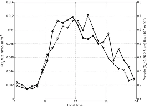
3.2 Diurnal cycles

Figure 3 shows a comparison of the diurnal cycles of aerosol particle flux (Dp, size range 0.25–2.5 µm) and CO₂fluxes for northerly winds (270 to 90◦_{). The aerosol fluxes}

15

are low in magnitude during nighttime and high during daytime. The CO₂fluxes show the same diurnal pattern with minimum values at night and highest during daytime with the maximum around midday being related both to increased human activity and more turbulent conditions. The median particle and CO₂ fluxes are always positive, which indicates that the city is mostly a net source for these parameters.

20

Aerosol and CO₂fluxes start to increase rapidly between 5 to 8 a.m. which correlates well with the morning tra_ffic rush hour. Both fluxes stay high during daytime. The decline in the evening around 6 p.m. is caused by a drop in traffic activity, which is main source for both CO₂ and aerosol within the footprint area. These observations are consistent with earlier studies in cities (Nemitz et al., 2002; Valesco et al., 2005;

25

(8)

ACPD

10, 21521–21545, 2010

M. Vogt et al.

Title Page

Tables Figures

◭ ◮

Back Close

Full Screen / Esc

Discussion

P

a

per

|

Dis

cussion

P

a

per

|

Discussion

P

a

per

|

Discussio

n

P

a

per

|

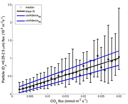
3.3 Emission factors

Particle EFs can be derived with di_fferent units depending on the available data and intended use. For example certain distance driven by a vehicle [g/km], or the amount of fuel burned [g/l], can be the fundament to quantify emissions of a certain substance. In our case CO₂is used as a tracer for road tra_ffic combustion.

5

A linear correlation between particle number flux and CO₂ flux was used to deter-mine an emission factor (Dp, size range 0.25–2.5 µm) in units of particles/mmol CO₂. Figure 4 shows the linear fit to the data. The data has been divided into 15 concentra-tion intervals. The interval width was chosen so that in each interval at least 20 or more half hour values were present. The linear fit was made to the median value of each size

10

bin. The slope of this fit has the units of [particles/mmol CO₂], which can be considered an emission factor. By converting mol into mass, EFs with units of [particle/g CO₂] can also be calculated. Note that the linear fit has been made only to the part of the data set with positive CO₂fluxes, as combustion does not consume CO₂.

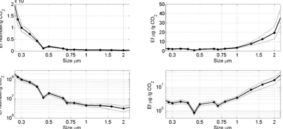
The combined linear fits to each of the 15 size channels of the OPC (Dp, size range

15

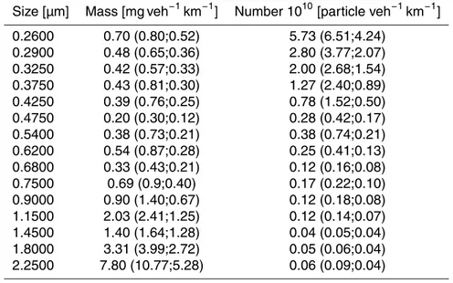
0.25–2.5 µm) gives size resolved EFs. By assuming a particle density of 1600 kg/m3 (Pitz et al., 2003) and using the particle sizes from the OPC, mass related emission factors [µg/g CO₂] may also be calculated (see Fig. 5). Even though Pitz et al. (2003) investigated that aerosol density showed pronounced diurnal pattern both in summer and in winter and also on weekdays and weekends, this hasn’t be taken into account

20

to keep the approach simple. Details of the EFs in mass and number can be found in Table 2. The number based emission factors have their highest values for the smallest aerosol sizes, while the mass based emission factors have the largest values in the super-micrometer range. Mass emissions below 0.75 µm Dp are close to constant with size, but show an exponential increase above this size.

(9)

ACPD

10, 21521–21545, 2010

M. Vogt et al.

Title Page

Tables Figures

◭ ◮

Back Close

Full Screen / Esc

Discussion

P

a

per

|

Dis

cussion

P

a

per

|

Discussion

P

a

per

|

Discussio

n

P

a

per

3.4 Comparable measurements and annual variation in emission factors

Comparable measurements have been made at a densely trafficked site (Hornsgatan with around 30 000 vehicles per day) in the city centre, in the northwest direction from of the tower. The measurements at Hornsgatan (a street canyon site previously described in detail by e.g. Gidhagen et al., 2005) were made using an OPC (Grimm Technologies,

5

Model 1.109), i.e. the same measurement technique and instrument as for the particle fluxes on the tower. The EFs obtained at Hornsgatan were calculated by using the NO_x scaling method. Thereby NO_xis used as a tracer. Detailed description can be found in Omstedt et al. (2005).

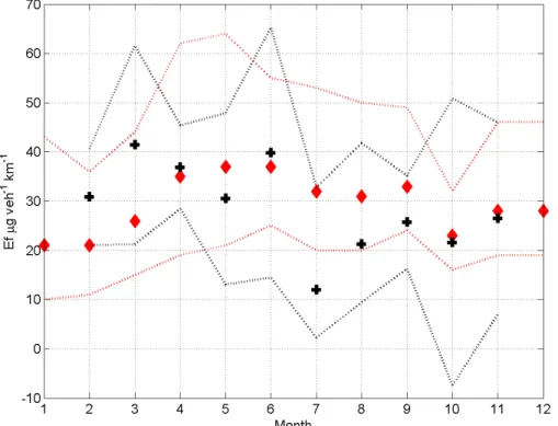
Figure 6 shows the annual variation in the EFs [mg veh−1_km−1_{] derived from}

10

the tower and the Hornsgatan measurements. To convert the EFs to the units of [veh−1_km−1_{] it was assumed that 90% of the cars in Stockholm run on gasoline fuel}

and 10% on diesel fuel and 95% of the cars are light duty tra_ffic and 5% heavy duty. In addition we assumed that light duty cars consume 0.1 l km−1_{of gasoline, 0.07 l km}−1_of

diesel and heavy duty vehicles 0.3 l km−1_{of diesel (SCM, Bayerisches Landesamt fuer}

15

Umwelt).

The EFs calculated from the communication tower correlate very well with those from Hornsgatan. Emission rates are generally higher in spring and early summer, than the rest of the year. The estimated emission factors and the variability of those for the tower-site and street-site overlap in most of the months except for July. Reasons for

20

that might be less traffic, which might lead to less break wear production. In addition the amount of heavy duty tra_ffic drops a lot during this period. The mean annual emission factor for Hornsgatan is 29.7 [mg veh−1_km−1_{] and 27.5 [mg veh}−1_km−1_{] for the tower}

(10)

ACPD

10, 21521–21545, 2010

M. Vogt et al.

Title Page

Tables Figures

◭ ◮

Back Close

Full Screen / Esc

Discussion

P

a

per

|

Dis

cussion

P

a

per

|

Discussion

P

a

per

|

Discussio

n

P

a

per

|

3.5 Relevant source processes and their influence on the emission factor

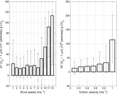
Gillette et al. (1982) showed the importance of turbulence for the suspension of course mode particles in deserts. As this is a process one could suspect it would apply on dust on roads as well, we attempted to investigate the e_ffect of di_fferent turbulent conditions on number EFs (Dp, size range 1–2.5 µm). Turbulence is produced either from heat

5

driving convection or wind shear near the ground shown in the friction velocity. Number EFs for seven di_fferent turbulence scenarios were calculated (friction velocity at the tower from 0.1 to 1.1 m s−1_{, see Fig. 7b). Figure 7b shows that the number emission}

factor is not significantly affected by turbulence for friction velocity conditions below 0.8 m s−1_{. Turbulent conditions over 0.8 m s}−1 _{show a large increase in the emission}

10

factor as the suspension of particles larger than 1 µm starts to become more e_ffective. The same analysis can be applied for the horizontal wind speed. Nemetz et al. (2001) found a dependence of the flux of coarse particles with horizontal wind speed similar to that shown in (7a). This indicates that coarse particles on roads or other ground surfaces may be suspended at high wind speeds. This is a well know phenomena

15

and has been shown for deserts (Fratini et al., 2007). Particles fluxes with a diameter smaller than 1.0 µm do not show this clear wind speed dependence (Nemetz et al., 2001). Because the mass EFs are dominated by particles in the size range (Dp, 1.0– 2.5 µm), it is anticipated that high winds will affect the particle mass flux. To test this hypothesis, the number EFs size range (Dp, 1.0–2.5 µm) were binned based on wind

20

speeds between 1 and 13 m s−1_{. We divided the wind speed into 11 bins to ensure that}

in each bin at least 20 values were present in each bin (see Fig. 7a).

From Fig. 7a, it appears that high wind speeds have a huge impact on the mass emission factor but the frequency of 30 min periods with wind speeds greater than 8 m s−1 _{appearing in our data set is around 5%, which means that these high wind}

25

(11)

ACPD

10, 21521–21545, 2010

M. Vogt et al.

Title Page

Tables Figures

◭ ◮

Back Close

Full Screen / Esc

Discussion

P

a

per

|

Dis

cussion

P

a

per

|

Discussion

P

a

per

|

Discussio

n

P

a

per

to high wind speed may influence extreme values and the amount of days that exceed critical levels especially if wind conditions coincide with high tra_ffic counts. This e_ffect should therefore be taken into account in air quality models. In conclusion, wind speed and friction velocity make a contribution on the aerosol flux and this is likely related to the fact that at higher wind speeds (or high u∗_{) particles sizes larger than 1.0 µm}

5

may become suspended. Since these high wind speeds were not common over the measurement period, vehicle induced turbulence and suspension of particles was likely to be the dominant process for large particle emissions.

3.6 Comparison of di_fferent methods to estimate emission factors

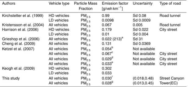
Table 2 gives an overview of PM_2.5 EFs in [g veh−1_km−_{1]. Emission factors range}

10

from 0.01 to 0.3 mg/vkm. Highest value is reported by Keogh. Differences between studies are to di_fferent contribution from exhaust and non-exhaust PM. Exhaust maybe due to di_fferent fleet mix HDV/LDV and di_fferent fuel mix (diesel/gasoline). Evaluating emission trends by comparing data with (Ketzel et al., 2007) is not very significant, as the contribution of exhaust emission, which may have decreased due to better catalyst

15

in cars from 2004 to 2008 is relatively small in Stockholm (Dp<0.6 µm). The major contribution to the total EFs of PM_2.5 here is mechanically produced particle matter (Dp>0.6 µm). Norman and Johansson discuss the fact that meteorology, and in partic-ular road wetness is the main parameter which controls PM_2.5 emissions (Norman et al., 2006). That being the case, the higher annual emission factor observed by Ketzel

20

in 2004 is likely due to a dry spring period.

(12)

ACPD

10, 21521–21545, 2010

M. Vogt et al.

Title Page

Tables Figures

◭ ◮

Back Close

Full Screen / Esc

Discussion

P

a

per

|

Dis

cussion

P

a

per

|

Discussion

P

a

per

|

Discussio

n

P

a

per

|

4 Summary and conclusion

Size-resolved vertical aerosol number fluxes of particles with Dp,=0.25–2.5 µm were measured with the eddy covariance method from a 105 m high communication tower over the city Stockholm, Sweden. In this study, size resolved number and mass EFs have been calculated and compared with other published results. In addition

meteoro-5

logical and special factors that may influence the EFs have been discussed. The key findings are

1. The highest values for the CO₂and particle flux are found to the Northeast.

2. Unlike the flux results, the maximum in particle concentration was found in the East to South (90 to 200◦_{), due to long range transport.}

10

3. Particle and CO₂fluxes show the same diurnal pattern with lows at night and highs during daytime with the maximum around midday being related both to increased human activity and more turbulent conditions.

4. Emission factors were determined by a linear correlation between particle number flux and CO₂flux.

15

5. Annual emission mass emission factor obtained with the eddy covariance method at the communication tower is slightly lower than that determined with the NO_x method in the street canyon (28, 30 [mg veh−1_km−1_]).

6. Emission rates are generally higher in spring than in summer.

7. Turbulent conditions over 0.8 m s−1 _{show a large increase in the emission factor}

20

as the suspension of particles larger than 1 µm starts to become more e_ffective.

(13)

ACPD

10, 21521–21545, 2010

M. Vogt et al.

Title Page

Tables Figures

◭ ◮

Back Close

Full Screen / Esc

Discussion

P

a

per

|

Dis

cussion

P

a

per

|

Discussion

P

a

per

|

Discussio

n

P

a

per

In conclusion CO₂fluxes in combination with particle fluxes can be used to derive EFs. The EFs in the size range of Dp,₌ 0.25–2.5 µm are a_ffected by high turbulence and high wind speed conditions due to resuspension of particles.

Acknowledgements. We would like to thank the Swedish Research Council for Environment,

Agricultural Science and Spatial Planning (FORMAS) and the Swedish Research Council (VR)

5

for supporting this project. We also acknowledge Leif B ¨acklin and Kai Rosman for technical assistance and Peter Tunved and Hamish Struthers for good discussions.

References

Areskoug, H., Camner, P., Dahlen, S. E., Lastbom, L., Nyberg, F., Pershagen, G., and Sydbom, A.: Particles in ambient air – a health risk assessment, Scand. J. Work. Env. Hea., 26, 1–96,

10

2000.

Buzorius, G., Rannik, U., Makela, J. M., Keronen, P., Vesala, T., and Kulmala, M.: Verti-cal aerosol fluxes measured by the eddy covariance method and deposition of nucleation mode particles above a Scots pine forest in southern Finland, J. Geophys. Res-Atmos., 105, 19905–19916, 2000.

15

Colberg, C. A., Tona, B., Stahel, W. A., Meier, M., and Staehelin, J.: Comparison of a road traffic emission model (HBEFA) with emissions derived from measurements in the Gubrist road tunnel, Switzerland, Atmos. Environ., 39, 4703–4714, 2005.

Coutts, A. M., Beringer, J., and Tapper, N. J.: Characteristics influencing the variability of urban CO2 fluxes in Melbourne, Australia, Atmos. Environ., 41, 51–62, 2007.

20

Dorsey, J. R., Nemitz, E., Gallagher, M. W., Fowler, D., Williams, P. I., Bower, K. N., and Beswick, K. M.: Direct measurements and parameterisation of aerosol flux, concentration and emission velocity above a city, Atmos. Environ., 36, 791–800, 2002.

Fratini, G., Ciccioli, P., Febo, A., Forgione, A., and Valentini, R.: Size-segregated fluxes of mineral dust from a desert area of northern China by eddy covariance, Atmos. Chem. Phys.,

25

7, 2839–2854, doi:10.5194/acp-7-2839-2007, 2007.

(14)

ACPD

10, 21521–21545, 2010

M. Vogt et al.

Title Page

Tables Figures

◭ ◮

Back Close

Full Screen / Esc

Discussion

P

a

per

|

Dis

cussion

P

a

per

|

Discussion

P

a

per

|

Discussio

n

P

a

per

|

Gidhagen, L., Johansson, C., Langner, J., and Foltescu, V. L.: Urban scale model-ing of particle number concentration in Stockholm, Atmos. Environ., 39, 1711–1725, doi:10.1016/j.atmosenv.2004.11.042, 2005.

Gillette, D. A., Adams, J., Endo, A., Smith, D., and Kihl, R.: Threshold Velocities for Input of Soil Particles into the Air by Desert Soils, J. Geophys. Res-Oc. Atm., 85, 5621–5630, 1980.

5

Grimmond, C. S. B., King, T. S., Cropley, F. D., Nowak, D. J., and Souch, C.: Local-scale fluxes of carbon dioxide in urban environments: methodological challenges and results from Chicago, Environ. Pollut., 116, 243–254, 2002.

Hall, E., Ramamurthy, S. S., and Balda, J. C.: Optimum speed ratio of induction motor drives for electrical vehicle propulsion, Appl. Power Elect. Co., 371–377, 1314, 2001.

10

Harrison, R. M., Shi, J. P., Xi, S. H., Khan, A., Mark, D., Kinnersley, R., and Yin, J. X.: Mea-surement of number, mass and size distribution of particles in the atmosphere, Philos. T. Roy Soc. A., 358, 2567–2579, 2000.

Horst, T. W.: A simple formula for attenuation of eddy fluxes measured with first-order-response scalar sensors, Bound-Lay. Meteorol., 82, 219–233, 1997.

15

Hueglin, C., Buchmann, B., and Weber, R. O.: Long-term observation of real-world road traffic emission factors on a motorway in Switzerland, Atmos. Environ., 40, 3696–3709, 2006. Jamriska, M. and Morawska, L.: A model for determination of motor vehicle emission factors

from on-road measurements with a focus on submicrometer particles, Sci. Total Environ., 264, 241–255, 2001.

20

J ¨arvi, L., Rannik, ¨U., Mammarella, I., Sogachev, A., Aalto, P. P., Keronen, P., Siivola, E., Kul-mala, M., and Vesala, T.: Annual particle flux observations over a heterogeneous urban area, Atmos. Chem. Phys., 9, 7847–7856, doi:10.5194/acp-9-7847-2009, 2009.

Keogh, D. U., Ferreira, L., and Morawska, L.: Development of a particle number and particle mass vehicle emissions inventory for an urban fleet, Environ. Modell Softw., 24, 1323–1331,

25

2009.

Kerminen, V. M., Pakkanen, T. A., Makela, T., Hillamo, R. E., Sillanpaa, M., Ronkko, T., Vir-tanen, A., Keskinen, J., Pirjola, L., Hussein, T., and Hameri, K.: Development of particle number size distribution near a major road in Helsinki during an episodic inversion situation, Atmos. Environ., 41, 1759–1767, 2007.

30

(15)

ACPD

10, 21521–21545, 2010

M. Vogt et al.

Title Page

Tables Figures

◭ ◮

Back Close

Full Screen / Esc

Discussion

P

a

per

|

Dis

cussion

P

a

per

|

Discussion

P

a

per

|

Discussio

n

P

a

per

Kirchstetter, T. W., Harley, R. A., Kreisberg, N. M., Stolzenburg, M. R., and Hering, S. V.: On-road measurement of fine particle and nitrogen oxide emissions from light- and heavy-duty motor vehicles, Atmos. Environ., 33, 2955–2968, 1999.

Kittelson, D. B., Watts, W. F., and Johnson, J. P.: Nanoparticle emissions on Minnesota high-ways, Atmos. Environ., 38, 9–19, 2004.

5

Kristensson, A., Johansson, C., Westerholm, R., Swietlicki, E., Gidhagen, L., Wideqvist, U., and Vesely, V.: Real-world traffic emission factors of gases and particles measured in a road tunnel in Stockholm, Sweden, Atmos. Environ., 38, 657–673, 2004.

Lenschow, D. H. and Raupach, M. R.: The Attenuation of Fluctuations in Scalar Concentrations through Sampling Tubes, J. Geophys. Res-Atmos., 96, 15259–15268, 1991.

10

M ˚artensson, E. M., Nilsson, E. D., Buzorius, G., and Johansson, C.: Eddy covariance measure-ments and parameterisation of traffic related particle emissions in an urban environment, Atmos. Chem. Phys., 6, 769–785, doi:10.5194/acp-6-769-2006, 2006.

Martin, C. L., Longley, I. D., Dorsey, J. R., Thomas, R. M., Gallagher, M. W., and Nemitz, E.: Ultrafine particle fluxes above four major European cities, Atmos. Environ., 43, 4714–4721,

15

2009.

McLaren, R., Gertler, A. W., Wittorff, D. N., Belzer, W., Dann, T., and Singleton, D. L.: Real-world measurements of exhaust and evaporative emissions in the Cassiar tunnel predicted by chemical mass balance modeling, Environ. Sci. Technol., 30, 3001–3009, 1996.

Nemitz, E., Fowler, D., Gallagher, M. W., Dorsey, J. R., Theobald, M. R., and Bower, K.:

Mea-20

surement and interpretation of land-atmosphere aerosol fluxes: current issues and new ap-proaches, edited by: Midgley, P. M., Reuther, M., and Williams, M., Proceedings of EURO-TRAC Symposium 2000, Springer Verlag Berlin, Heidelberg, 45–53, 2001.

Nemitz, E., Hargreaves, K. J., McDonald, A. G., Dorsey, J. R., and Fowler, D.: Meteorological measurements of the urban heat budget and CO2 emissions on a city scale, Environ. Sci.

25

Technol., 36, 3139–3146, 2002.

Norman, M. and Johansson, C.: Studies of some measures to reduce road dust emissions from paved roads in Scandinavia, Atmos. Environ., 40, 6154–6164, 2006.

Omstedt, G., Bringfelt, B., and Johansson, C.: A model for vehicle-induced non-tailpipe emis-sions of particles along Swedish roads, Atmos. Environ., 39, 6088–6097, 2005.

30

(16)

ACPD

10, 21521–21545, 2010

M. Vogt et al.

Title Page

Tables Figures

◭ ◮

Back Close

Full Screen / Esc

Discussion

P

a

per

|

Dis

cussion

P

a

per

|

Discussion

P

a

per

|

Discussio

n

P

a

per

|

Brunekreef, B., Wichmann, H. E., Buzorius, G., Vallius, M., Kreyling, W. G., and Pekkanen, J.: Concentrations of ultrafine, fine and PM2.5 particles in three European cities, Atmos. Environ., 35, 3729–3738, 2001.

Sjodin, A. and Lenner, M.: On-Road Measurements of Single Vehicle Pollutant Emissions, Speed and Acceleration for Large Fleets of Vehicles in Different Traffic Environments, Sci.

5

Total Environ., 169, 157–165, 1995.

Sjogren, M., Li, H., Banner, C., Rafter, J., Westerholm, R., and Rannug, U.: Influence of physical and chemical characteristics of diesel fuels and exhaust emissions on biological effects of particle extracts: A multivariate statistical analysis of ten diesel fuels, Chem. Res. Toxicol., 9, 197–207, 1996.

10

Tunved, P., Nilsson, E. D., Hansson, H.-C., and Str ¨om, J.: Aerosol characteristics of air masses in northern Europe: Influences of location, transport, sinks, and sources, J. Geophys. Res. 110, D07201, doi:10.1029/2004JD005085, 2005.

Velasco, E., Pressley, S., Allwine, E., Westberg, H., and Lamb, B.: Measurements of CO2 fluxes from the Mexico City urban landscape, Atmos. Environ., 39, 7433–7446, 2005.

15

Vogt, M., Nilsson, E.D., Ahlm, L., M ˚artensson, M., and Johansson, C.: Seasonal and diurnal cycles of 0.25-2.5µm aerosol and CO2 fluxes over urban Stockholm, Sweden, Tellus B, in

review, 2010.

Vogt, R., Christen, A., Rotach, M. W., Roth, M., and Satyanarayana, A. N. V.: Temporal dy-namics of CO2 fluxes and profiles over a central European city, Theor. Appl. Climatol., 84,

20

117–126, 2006.

Webb, E. K., Pearman, G. I., and Leuning, R.: Correction of Flux Measurements for Density Effects Due to Heat and Water-Vapor Transfer, Q. J. Roy. Meteor. Soc., 106, 85–100, 1980. Westerholm, R. and Egeback, K. E.: Exhaust Emissions from Light-Duty and Heavy-Duty

Ve-hicles – Chemical-Composition, Impact of Exhaust after Treatment, and Fuel Parameters,

25

(17)

ACPD

10, 21521–21545, 2010

M. Vogt et al.

Title Page

Tables Figures

◭ ◮

Back Close

Full Screen / Esc

Discussion

P

a

per

|

Dis

cussion

P

a

per

|

Discussion

P

a

per

|

Discussio

n

P

a

per

Table 1.Median mass and number emission factor for each of the 15 OPC size bins. Values in brackets represent the 95% confidence interval.

Size [µm] Mass [mg veh−1_km−1_] _{Number 10}10_{[particle veh}−1_km−1_]

(18)

ACPD

10, 21521–21545, 2010

M. Vogt et al.

Title Page

Tables Figures

◭ ◮

Back Close

Full Screen / Esc

Discussion

P

a

per

|

Dis

cussion

P

a

per

|

Discussion

P

a

per

|

Discussio

n

P

a

per

|

Table 2.Published emission factors for particulate mass fractions on road studies.

Authors Vehicle type Particle Mass Emission factor Uncertainty Type of road Fraction [g/veh km−1_]

Kirchstetter et al. (1999) HD vehicles PM₂.5 0.99 Sd 0.08 Road tunnel LD vehicles PM₂.5 0.0098 Sd 0.0009

Kristensson et al. (2004) All vehicles PM₂.5 0.067 0.005 Road tunnel Harrison et al. (2006) HD vehicles PM₂_.₅ 0.179 Sd 0.022 City street

LD vehicles PM₂.5 0.01 Sd 0.004

Grieshop et al. (2006) All vehicles PM₂_.₅ 0.022 (213)a Sd 31 Cheng et al. (2009) All vehicles PM₂.5 0.131 Sd 0.0369 Ketzel et al. (2007) All vehicles PM₂.5 0.054

b

Not available All vehicles PM₂.5 0.067

c

Not available City street All vehicles PM₂.5 0.029

d

Not available City street All vehicles PM₂.5 0.033

e

Not available City street Keogh et al. (2009) HD vehicles PM₂.5 0.302

LD vehicles PM₂_.₅ 0.033

This study All vehicles PM₂_.₅ 0.030f (0.018,0.48) Street Canyon All vehicles PM₂_.₅ 0.028g (0.013,0.45) Tower(EC)

a

Emission factor in unit [mg (kg fuel−1_{)] (original value).}

b

Measurements made at H.C Andersens Blvd in in Copenhagen, Denmark (2003–2004). c

Measurements made at Hornsgatan in Stockholm, Sweden (2002–2004). d_{Measurements made at Merseburger Strasse, Halle, Germany (2003–2004).} e

Measurements made at Runbergkatu, Helsinki, Finnland (2003–2004). f_{Measurements made at Hornsgatan in Stockholm, Sweden (2008–2009).} g

(19)

ACPD

10, 21521–21545, 2010

M. Vogt et al.

Title Page

Tables Figures

◭ ◮

Back Close

Full Screen / Esc

Discussion

P

a

per

|

Dis

cussion

P

a

per

|

Discussion

P

a

per

|

Discussio

n

P

a

per

(20)

ACPD

10, 21521–21545, 2010

M. Vogt et al.

Title Page

Tables Figures

◭ ◮

Back Close

Full Screen / Esc

Discussion

P

a

per

|

Dis

cussion

P

a

per

|

Discussion

P

a

per

|

Discussio

n

P

a

per

|

Fig. 2. (a)Aerosol number and CO2flux and(b)particle and CO2 concentrations in constant

wind sector intervals. Bars represent CO2flux and concentrations. Solid line: aerosol number

(21)

ACPD

10, 21521–21545, 2010

M. Vogt et al.

Title Page

Tables Figures

◭ ◮

Back Close

Full Screen / Esc

Discussion

P

a

per

|

Dis

cussion

P

a

per

|

Discussion

P

a

per

|

Discussio

n

P

a

per

(22)

ACPD

10, 21521–21545, 2010

M. Vogt et al.

Title Page

Tables Figures

◭ ◮

Back Close

Full Screen / Esc

Discussion

P

a

per

|

Dis

cussion

P

a

per

|

Discussion

P

a

per

|

Discussio

n

P

a

per

|

Fig. 4.Median values for particles particle flux with Dp=0.25–2.5 µm within constant intervals

of CO2flux. The vertical bars represent 25 and 75 percentiles. The blue line represents the

(23)

ACPD

10, 21521–21545, 2010

M. Vogt et al.

Title Page

Tables Figures

◭ ◮

Back Close

Full Screen / Esc

Discussion

P

a

per

|

Dis

cussion

P

a

per

|

Discussion

P

a

per

|

Discussio

n

P

a

per

(24)

ACPD

10, 21521–21545, 2010

M. Vogt et al.

Title Page

Tables Figures

◭ ◮

Back Close

Full Screen / Esc

Discussion

P

a

per

|

Dis

cussion

P

a

per

|

Discussion

P

a

per

|

Discussio

n

P

a

per

|

Fig. 6. Monthly median emission factors (red, triangle) street canyon, using the NOx method

(25)

ACPD

10, 21521–21545, 2010

M. Vogt et al.

Title Page

Tables Figures

◭ ◮

Back Close

Full Screen / Esc

Discussion

P

a

per

|

Dis

cussion

P

a

per

|

Discussion

P

a

per

|

Discussio

n

P

a

per