Modeling global atmospheric CO<sub>2</sub> with improved emission inventories and CO<sub>2</sub> production from the oxidation of other carbon species

(1)

GMDD

3, 889–948, 2010

Modeling CO₂with improved inventories

and chemical production

R. Nassar et al.

Title Page

Abstract Introduction

Conclusions References

Tables Figures

◭ ◮

Back Close

Full Screen / Esc

Printer-friendly Version Interactive Discussion

Discussion

P

a

per

|

Dis

cussion

P

a

per

|

Discussion

P

a

per

|

Discussio

n

P

a

per

Geosci. Model Dev. Discuss., 3, 889–948, 2010 www.geosci-model-dev-discuss.net/3/889/2010/ doi:10.5194/gmdd-3-889-2010

Geoscientific Model Development Discussions

This discussion paper is/has been under review for the journal Geoscientific Model Development (GMD). Please refer to the corresponding final paper in GMD if available.

Modeling global atmospheric CO

₂

with

improved emission inventories and CO

₂

production from the oxidation of other

carbon species

R. Nassar1,2, D. B. A. Jones1, P. Suntharalingam3, J. M. Chen2, R. J. Andres4, K. J. Wecht5, R. M. Yantosca6, S. S. Kulawik7, K. W. Bowman7, J. R. Worden7, T. Machida8, and H. Matsueda9

1

Department of Physics, University of Toronto, 60 St. George Street, Toronto, Ontario, M5S 1A7, Canada

2

Department of Geography, University of Toronto, 45 St. George Street, Toronto, Ontario, M5S 2E5, Canada

3

Environmental Sciences, University of East Anglia, Norwich, NR4 7TJ, UK

4

Environmental Sciences Division, Oak Ridge National Laboratory, Oak Ridge, TN, 37831-6335, USA

5

(2)

GMDD

3, 889–948, 2010

R. Nassar et al.

Title Page

Tables Figures

◭ ◮

Back Close

Full Screen / Esc

Discussion

P

a

per

|

Dis

cussion

P

a

per

|

Discussion

P

a

per

|

Discussio

n

P

a

per

|

6

School of Engineering and Applied Sciences, Harvard University, Pierce Hall, 29 Oxford St., Cambridge, MA, 02138, USA

7

Jet Propulsion Laboratory, California Institute of Technology, 4800 Oak Grove Drive, Pasadena, CA, 91109, USA

8

National Institute for Environmental Studies, 16-2 Onogawa, Tsukuba-City, Ibaraki, 305-8506, Japan

9

Meteorological Research Institute, 1-1 Nagamine, Tsukuba-city, Ibaraki 305-0052, Japan Received: 5 June 2010 – Accepted: 14 June 2010 – Published: 2 July 2010

Correspondence to: R. Nassar (ray.nassar@utoronto.ca)

(3)

GMDD

3, 889–948, 2010

R. Nassar et al.

Title Page

Tables Figures

◭ ◮

Back Close

Full Screen / Esc

Discussion

P

a

per

|

Dis

cussion

P

a

per

|

Discussion

P

a

per

|

Discussio

n

P

a

per

Abstract

The use of global three-dimensional (3-D) models with satellite observations of CO₂in inverse modeling studies is an area of growing importance for understanding Earth’s carbon cycle. Here we use the GEOS-Chem model (version 8-02-01) CO₂ simula-tion with multiple modificasimula-tions in order to assess their impact on CO₂forward simula-5

tions. Modifications include CO₂surface emissions from shipping (∼0.19 Pg C/yr), 3-D spatially-distributed emissions from aviation (_∼0.16 Pg C/yr), and 3-D chemical produc-tion of CO₂ (∼1.05 Pg C/yr). Although CO2 chemical production from the oxidation of CO, CH₄ and other carbon gases is recognized as an important contribution to global CO₂, it is typically accounted for by conversion from its precursors at the surface rather 10

than in the free troposphere. We base our model 3-D spatial distribution of CO₂ chemi-cal production on monthly-averaged loss rates of CO (a key precursor and intermediate in the oxidation of organic carbon) and apply an associated surface correction for in-ventories that have counted emissions of carbon precursor as CO₂. We also explore the benefit of assimilating satellite observations of CO into GEOS-Chem to obtain an 15

observation-based estimate of the CO₂ chemical source. The CO assimilation cor-rects for an underestimate of atmospheric CO abundances in the model, resulting in increases of as much as 24% in the chemical source during May–June 2006, and in-creasing the global annual estimate of CO₂chemical production from 1.05 to 1.18 Pg C. Comparisons of model CO₂ with measurements are carried out in order to investigate 20

the spatial and temporal distributions that result when these new sources are added. Inclusion of CO₂emissions from shipping and aviation are shown to increase the global CO₂latitudinal gradient by just over 0.10 ppm (∼3%), while the inclusion of CO2 chem-ical production (and the surface correction) is shown to decrease the latitudinal gra-dient by about 0.40 ppm (_∼10%) with a complex spatial structure generally resulting 25

(4)

GMDD

3, 889–948, 2010

R. Nassar et al.

Title Page

Tables Figures

◭ ◮

Back Close

Full Screen / Esc

Discussion

P

a

per

|

Dis

cussion

P

a

per

|

Discussion

P

a

per

|

Discussio

n

P

a

per

|

1 Introduction

An important application of global three-dimensional (3-D) modeling of atmospheric carbon dioxide (CO₂) is the assimilation of CO₂ observations to obtain optimized es-timates of atmospheric CO₂ distributions or CO₂ surface fluxes (sources and sinks). The optimization of CO₂fluxes (also referred to as inverse modeling) has mainly been 5

carried out using in situ or flask observations obtained near the surface of the Earth, but in recent years, many studies have explored the potential of inverse modeling using satellite observations (Pak and Prather, 2001; Rayner and O’Brien, 2001; Houweling et al., 2004; Miller et al., 2007, Chevallier et al., 2007; Kadygrov et al., 2009). A sig-nificant challenge with the inverse modeling approach is that inferred flux estimates 10

are sensitive to systematic errors in the models and observations (Miller et al., 2007; Chevallier et al., 2007; Kadygrov et al., 2009) and since satellite observations measure atmospheric columns or profiles rather than point measurements at the Earth’s sur-face, the 3-D representation of CO₂in the model is of increased importance. Reducing spatially-dependent biases in the models requires not only a better representation of 15

atmospheric transport and surface sources and sinks of CO₂, but also the inclusion of 3-D sources distributed throughout the troposphere, such as emission of CO₂ from aviation and the chemical production of CO₂from the oxidation of CO, CH₄ and other organic gases. The importance of accounting for this tropospheric chemical source of CO₂ in models has previously been acknowledged (Enting and Mansbridge, 1991; 20

Enting et al., 1995; Baker, 2001; Enting, 2004; Folberth et al., 2005; Suntharalingam et al., 2005; Denman et al., 2007, Ch. 7 IPCC-AR4). To balance atmospheric CO₂in the absence of this 3-D chemical source, many inventories count CO₂ precursor species (CO, CH₄and other carbon gases) as direct CO₂emissions at the surface, leading to a reasonable estimate of total CO₂over time, but an incorrect spatial distribution, since 25

(5)

GMDD

3, 889–948, 2010

R. Nassar et al.

Title Page

Tables Figures

◭ ◮

Back Close

Full Screen / Esc

Discussion

P

a

per

|

Dis

cussion

P

a

per

|

Discussion

P

a

per

|

Discussio

n

P

a

per

chemical production of CO₂ is greatest in the tropics, while most surface emissions occur in the Northern Hemisphere, the combined chemical production and surface correction will have an impact on the global latitudinal gradient of CO₂, which is an indentified weakness of CO₂ models (Law et al., 1996; Taylor and Orr, 2000; Gurney et al., 2003) and consequently could a_ffect inverse estimates of CO₂fluxes.

5

In this work, we use the GEOS-Chem CO₂ simulation with multiple modifications applied to investigate the impact of these changes on atmospheric CO₂ distributions. This work is motivated by our objective of improving CO₂forward simulations for use in inverse modeling with satellite observations of CO₂. Our modifications to the CO₂ simu-lation include improved temporal variability in the national surface fossil fuel combustion 10

and cement manufacture inventory, the addition of surface CO₂ emissions from ship-ping, 3-D CO₂ emissions from domestic and international aviation, and 3-D chemical production of CO₂from the oxidation of reduced carbon species, along with an associ-ated surface correction. Although a small number of past forward or inverse modeling studies have included CO₂chemical production (Enting and Mansbridge, 1991, Enting 15

et al., 1995, Baker, 2001), to the best of our knowledge, our modifications result in the most comprehensive online model representation of 3-D CO₂chemical production and the appropriate surface correction in forward simulations. Use of the resulting model distributions in inverse analyses enables a significant reduction in the systematic error introduced into surface CO₂ flux estimates through the misallocation of the reduced 20

carbon fluxes. We base our CO₂ chemical source on the rates of conversion of CO to CO₂from a GEOS-Chem simulation of tropospheric ozone-hydrocarbon chemistry. We also briefly explore the assimilation of satellite observations of CO from the Tropo-spheric Emission Spectrometer (TES) into GEOS-Chem to produce an optimized CO distribution, from which we obtain an observationally-based estimate of the chemical 25

production of CO₂.

(6)

GMDD

3, 889–948, 2010

R. Nassar et al.

Title Page

Tables Figures

◭ ◮

Back Close

Full Screen / Esc

Discussion

P

a

per

|

Dis

cussion

P

a

per

|

Discussion

P

a

per

|

Discussio

n

P

a

per

|

measurements (Matsueda et al., 2002, 2008; Machida et al., 2008). It is important to emphasize that in this work we have focused our model improvement e_fforts on better representing emissions related to fossil fuel use (on land, from shipping, aviation, and chemical production related to emission of CO₂ precursors), rather than addressing the representation of biospheric CO₂ fluxes in the model. This choice was deliberate, 5

since CO₂ inverse modeling studies typically fix fossil fuel emissions assuming highly accurate inventories, while land biospheric CO₂ fluxes (which have larger uncertain-ties) are optimized using inverse modeling. This approach is currently being applied to our inverse modeling to obtain improved biospheric flux estimates using CO₂ obser-vations from the TES satellite instrument and from the surface observational network 10

(Nassar et al., 2010).

2 GEOS-Chem CO₂simulation

GEOS-Chem is a global chemical transport model (CTM) that uses GEOS (Goddard Earth Observing System) assimilated meteorological fields from the NASA Global Mod-eling and Assimilation O_ffice (GMAO). The model has multiple separate simulation 15

modes, the most common of which is the O_x-NO_x-hydrocarbon chemistry or “full chem-istry” mode (Bey et al., 2001). This mode has been extensively validated using in situ and satellite observations (e.g., Li et al., 2004; Folkins et al., 2006; Nassar et al., 2009, Kopacz et al., 2010, Millet et al., 2010). An early version of the CO₂ mode is described in Suntharalingam et al. (2004), which contained no chemistry but included 20

atmospheric CO₂fluxes from biomass burning, biofuel burning, fossil fuel burning and cement manufacture, ocean exchange and terrestrial biospheric exchange described in Suntharalingam et al. (2003). Previous application of this version of the model for inverse modeling of atmospheric CO₂ is described in Palmer et al. (2006), Miller et al. (2007), Feng et al. (2009), and Wang et al. (2009). In this work, we use version 25

(7)

GMDD

3, 889–948, 2010

R. Nassar et al.

Title Page

Tables Figures

◭ ◮

Back Close

Full Screen / Esc

Discussion

P

a

per

|

Dis

cussion

P

a

per

|

Discussion

P

a

per

|

Discussio

n

P

a

per

2.1 Fossil fuel burning and cement manufacture

The original version of the GEOS-Chem CO₂simulation used global annual emissions of CO₂ from fossil fuels and cement manufacture for 1995 at 1◦×1◦resolution (Andres

et al., 1996), regridded o_ffline to the GEOS grids. The inventory was developed at the Carbon Dioxide Information and Analysis Centre (CDIAC) of the Oak Ridge National 5

Laboratory (ORNL) based on reported national CO₂emissions for 186 countries, which were spatially distributed using detailed population statistics (United Nations, 1984) and national political boundaries from the Goddard Institute for Space Studies (GISS). The earlier version of the inventory corresponded to the first year of each decade from 1950–1990 but has since been expanded and improved such that the current ver-10

sion spans 1950–2006, providing monthly emission totals to account for the di_ffering regional seasonal variability of fossil fuel use related to climate and economic fac-tors (Andres et al., 2010). This updated inventory is important since global fossil fuel emissions have been increasing significantly since the 1990s, contributing 8.23 Pg C in 2006. Also included in this inventory is the non-fossil fuel production of CO₂ from 15

cement manufacture, which occurs via the conversion of CaCO₃to CaO+CO₂, repre-senting about 5% of total emissions in the inventory, but a larger proportion in China, the world’s highest emitting nation.

Figure 1 shows monthly surface CO₂comparisons between GEOS-Chem runs with monthly and annually varying fossil fuel emissions, starting from the same initial con-20

ditions. The monthly-varying emissions lead to more CO₂in the Northern Hemisphere (NH) in the first few months of the year, driven by high fossil fuel use in Europe, Canada and the Northern United States, presumably related to winter heating. Although the dif-ference during the NH winter is largest over northern populated areas where it exceeds 1 ppm, the background CO₂is also elevated by about 0.1 ppm from 30–90◦N in March. 25

(8)

GMDD

3, 889–948, 2010

R. Nassar et al.

Title Page

Tables Figures

◭ ◮

Back Close

Full Screen / Esc

Discussion

P

a

per

|

Dis

cussion

P

a

per

|

Discussion

P

a

per

|

Discussio

n

P

a

per

|

remain below their annual mean, while the US northeast is slightly above, presumably due to elevated energy consumption from air-conditioning use. In early September and October, NH CO₂is lower than the annual average (nearly mirroring March and April) since energy consumption due to heating and cooling reaches an annual minimum. At the end of the year, the run with monthly emissions returns to higher CO₂values over 5

Europe and the US. The observed seasonality over China is markedly different from other high-emitting regions. Rather than exhibiting the cyclical pattern of Europe, the US and Canada, a near-constant increase is the dominant form of change observed over China. The increase in CO₂ emissions from China over the course of a single year, captured by the monthly inventory (but not the annual one) has an impact compa-10

rable in magnitude to the seasonal cycle from other high-emitting regions. Therefore, in addition to masking the seasonality of emissions (related to seasonally-varying energy consumption based on heating and air conditioning), an annual rather than monthly inventory would represent the fairly constant increase in CO₂ emissions from China (Gregg et al., 2008) as an unrealistically abrupt jump on 1 January of each year. 15

Overall, this comparison indicates that a fossil fuel inventory based on monthly totals rather than annual totals has an impact often exceeding 1.0 ppm near the surface over regions of high fossil fuel consumption (Europe, US, Canada and China). Away from the source regions, the impact is muted, decreasing to about 0.1 ppm across the NH. The di_fferences are negligible in the tropics and Southern Hemisphere (SH).

20

Preliminary fossil fuel data are available for 2007 and 2008 for major emitting coun-tries on the CDIAC website, based on BP energy statistics. These preliminary values were used to scale the monthly spatial distributions of 2006 based on the ratios of estimates for these years to 2006 values, such that the seasonality in the emissions remains unchanged. Ratios were applied at the national level for the United States, 25

(9)

GMDD

3, 889–948, 2010

R. Nassar et al.

Title Page

Tables Figures

◭ ◮

Back Close

Full Screen / Esc

Discussion

P

a

per

|

Dis

cussion

P

a

per

|

Discussion

P

a

per

|

Discussio

n

P

a

per

2007, so we apply scaling factors for 2009 based on scaling factors for 2007, except for the US, Australia and China. US emissions decreased by 3.1% from 2007 to 2008, so, we apply a similar decrease for 2009. Australia’s emission also decreased from 2007 to 2008, so we simply apply the lower 2008 values. China’s emissions increased by 15.5% from 2006 to 2008 roughly equally for both years, but to balance the total sum 5

of all nations, we reduced 2009 emissions from China to 9% above 2006 levels.

2.2 Biomass burning

Biomass burning includes the burning of vegetation induced by natural processes like lightning as well as anthropogenically-induced burning, a common method of clearing vegetation for agriculture or urbanization. GEOS-Chem can be run with climatologi-10

cal, seasonally-varying biomass burning emissions (Duncan et al., 2003) or the much preferred year-specific Global Fire Emission Database version 2 (GFEDv2) (van der Werf et al., 2006). The GFEDv2 approach is to apply a CO₂emission factor for a given vegetation type (savanna, tropical forest, extratropical forest) to a fuel load and burned area determined from MODIS (Moderate Resolution Imaging Spectroradiometer) 8-15

day fire counts (Giglio et al., 2003). GFEDv2 CO₂emission data are provided at 1◦

×1◦

and regridded during a GEOS-Chem simulation. GFEDv2 is available as monthly av-erages (1997–2008) or 8-day avav-erages (2001–2007). The mean global annual CO₂ in GFEDv2 (1997–2008) is 2.35 Pg C/yr (approximately 30% of CO₂ from fossil fuel combustion), thus it represents a significant source of CO₂.

20

2.3 Biofuel burning

Biofuel burning in this context refers to the anthropogenic burning of vegetation for heating, cooking and removal of agricultural waste, mostly in developing countries. The model uses annual mean biofuel CO₂ emissions from Yevich and Logan (2003) with a native resolution of 1◦

×1◦. The global annual sum of the biofuel CO2 emis-25

(10)

GMDD

3, 889–948, 2010

R. Nassar et al.

Title Page

Tables Figures

◭ ◮

Back Close

Full Screen / Esc

Discussion

P

a

per

|

Dis

cussion

P

a

per

|

Discussion

P

a

per

|

Discussio

n

P

a

per

|

from agricultural burning in fields is not included since this is better represented by GFED, yielding 0.73 Pg C. We scale 1985 values to 1995 according to Yevich and Lo-gan (2003), giving a total without burning in fields of 0.80 Pg C. Growth patterns of global biofuel emissions beyond 1995 are unclear, but a steady increase is unlikely due to a shift to fossil fuels in the developing world as urbanization increases. No di-5

urnal or seasonal variability or trends in biofuel emissions are included, but since the biofuel contribution is small relative to other sources, the error in assuming constant emissions from 1995 should also be small.

2.4 Terrestrial biospheric exchange

Terrestrial biospheric exchange in the model consists of two components. The first is 10

referred to as the “balanced biosphere” and is based on the Carnegie-Ames-Stanford-Approach (CASA) model (Potter et al., 1993, Randerson et al., 1997). For the specific CASA run used here (Olsen and Randerson, 2004), the sum of the Gross Primary Production (GPP) and ecosystem respiration (R_e) is taken to represent Net Ecosystem Productivity (NEP) for 2000. Monthly mean NEP fluxes from CASA were interpolated to 15

daily values and balanced such that they give no net annual uptake/release of CO₂. In balancing the CASA fluxes, the net global contribution from the field is set to 0 Pg C/yr in order to represent terrestrial fluxes with no anthropogenic interference. These CASA balanced biosphere fluxes implicitly account for the natural cycle of non-respiratory carbon losses from the biosphere such as fires, methane and NMVOCs, and leaching 20

of soil organic carbon (Randerson et al., 2002). The CASA NEP output is used as Net Ecosystem Exchange (NEE) in our model simulation. Although these NEE balanced biosphere fluxes contribute no net annual uptake/release of CO₂by design, they make the largest contribution to the seasonal cycle of atmospheric CO₂ over both land and ocean over most of the globe with the greatest impacts (largest amplitude) seen in the 25

(11)

GMDD

3, 889–948, 2010

R. Nassar et al.

Title Page

Tables Figures

◭ ◮

Back Close

Full Screen / Esc

Discussion

P

a

per

|

Dis

cussion

P

a

per

|

Discussion

P

a

per

|

Discussio

n

P

a

per

A second component for CO₂resulting from terrestrial biospheric exchange is nec-essary to account for the total annual sum of biospheric uptake and emission of CO₂, which we refer to as the residual annual terrestrial exchange. This biospheric flux term is commonly the state to be optimized in inverse modeling. To provide a good a pri-ori description of this residual annual terrestrial exchange for inverse modeling, we 5

have incorporated into the model a climatology of inversion results from TransCom 3 (Baker et al., 2006), applied for the 11 TransCom land regions, as shown in Fig. 2. In TransCom, the residual annual biospheric flux is defined to include GPP andR_eas well as biomass burning, unlike in GEOS-Chem where burning is primarily specified sepa-rately. Since biofuel emissions were not explicitly dealt with in the TransCom inversions, 10

they will also have been implicitly included in their residual annual terrestrial exchange. To account for this, we subtract a GFEDv2 climatology and 1995 biofuel burning emis-sions from the TransCom climatology to obtain an estimate of the NEE component only. The TransCom climatology spans the years 1991–2000. For the GFED climatology, we use 1997–2006, thus both decade-long periods include the strong Southeast Asian 15

biomass burning event related to the 1997–1998 El Ni ˜no, that resulted in global CO₂ emissions that were 23% higher than average in 1997 and 30% higher in 1998, with a standard deviation of 15% for the 1997–2006 period. Biomass burning emissions were available from GFEDv2 for 2007–2008, but these were left out of the climatology to avoid “dilution” of the strong El Ni ˜no signal in one climatology but not the other. 20

With the climatological approach to terrestrial biospheric fluxes, the problem of double-counting natural biomass burning processes (which are in both CASA and GFED), is mitigated since the inversion result optimizes the sum of these terms. An acknowledged weakness in this climatological approach is the gradual downward trend in global biomass burning emissions in GFED over this time period, coupled with the 25

(12)

GMDD

3, 889–948, 2010

R. Nassar et al.

Title Page

Tables Figures

◭ ◮

Back Close

Full Screen / Esc

Discussion

P

a

per

|

Dis

cussion

P

a

per

|

Discussion

P

a

per

|

Discussio

n

P

a

per

|

The direct TransCom climatology gives an average of−2.09 Pg C/yr for residual

ter-restrial sinks, the GFED climatology gives an average of ₊2.39 Pg C/yr, and biofuel emissions were+0.80 Pg C/yr, which combined give us a climatology with a global to-tal of−5.29 Pg C/yr (Fig. 2). Relative to net annual terrestrial exchange in the previous

version of GEOS-Chem, the climatology has an opposite sign for the flux over Temper-5

ate North America (now a sink as shown by others) and Tropical America goes from near neutral to a source. The performance of the forward model with this a priori annual net exchange is evaluated in Sect. 3 and its performance in inverse modeling will be evaluated in Nassar et al. (2010).

2.5 Ocean exchange

10

GEOS-Chem simulates ocean release and uptake of CO₂ using ocean climatologies. The original GEOS-Chem CO₂ simulation relied on the ocean climatology from Taka-hashi et al. (1997), which was based on about 250 000 non-El Ni ˜no measurements of the pressure of CO₂ dissolved in ocean water (pCO₂), globally interpolated to an an-nual mean 4◦

×5◦ocean grid, with a unit conversion (to molecules of CO2cm−2s−1) ap-15

plied and regridded to the GEOS grids. An improved version of the ocean climatology with monthly variability was later developed (Takahashi et al., 2002). The most recent version, based on 3 million non-El Ni ˜nopCO₂measurements (Takahashi et al., 2009) has now been implemented in GEOS-Chem, with the option of selecting an annual mean or monthly-varying climatology. The tropical oceans (especially the Equatorial 20

Eastern Pacific) are generally a CO₂ source, while the mid- and high latitude oceans (especially the North Atlantic) are generally a CO₂ sink. The main exceptions are CO₂source regions along the Antarctic sea ice-ocean boundary and a small, variable source near the Bering Sea. The new climatology indicates a net global annual air-sea flux of 1.4±0.3 Pg C/yr, a somewhat stronger sink estimate than that from the 1997 25

(13)

GMDD

3, 889–948, 2010

R. Nassar et al.

Title Page

Tables Figures

◭ ◮

Back Close

Full Screen / Esc

Discussion

P

a

per

|

Dis

cussion

P

a

per

|

Discussion

P

a

per

|

Discussio

n

P

a

per

Jacobson et al., 2007a) for comparing with ocean carbon sink estimates, but other es-timates of the global riverine component are as high as 0.90 Pg C/yr (Cole et al., 2007). The riverine carbon contribution to the ocean is only significant when comparing air-sea flux with ocean carbon sinks, since this indirect transfer of atmospheric carbon to the ocean via the land, is treated as a component of the land sink in GEOS-Chem. 5

2.6 Shipping and aviation

Due the fact that the national CO₂ emission sums that are spatially distributed in the CDIAC 1◦×1◦ inventory (Andres et al., 1996) are primarily intended to show national

origin of emissions, the inventory does not include CO₂ emissions from bunker fu-els. These fuels are considered international (not associated with any specific nation) 10

since they are predominantly used for international shipping and aviation. (One excep-tion is the CO₂ emission from Antarctic fisheries, which is treated as a separate na-tional inventory.) For example, global annual CO₂ emissions from fossil fuels in 2006 (from CDIAC) amounted to 8.230 Pg C, but the sum of national emissions amounted to 7.828 Pg C yielding a di_fference of 0.402 Pg C of which 0.255 Pg C is attributed to 15

bunker fuels. The remainder of the di_fference primarily relates to non-combustion uses of fossil fuels such as the chemical production of plastics, with a smaller contribution (positive or negative) from changes in fuel reserves from year to year.

Accounting for CO₂ emissions from shipping and aviation in the model requires knowledge of both the quantity and spatial distribution of emissions. The spatial distri-20

bution of shipping emissions based on the Emissions Database for Global Atmospheric Research (EDGAR) inventory (Olivier and Berdowsky, 2001) is now an option for CO₂ (as for other chemical species in GEOS-Chem), but it contains a largely simplified representation of shipping routes. EDGAR, the Automated Mutual-assistance Vessel Rescue system (AMVER) and the International Comprehensive Ocean-Atmosphere 25

(14)

GMDD

3, 889–948, 2010

R. Nassar et al.

Title Page

Tables Figures

◭ ◮

Back Close

Full Screen / Esc

Discussion

P

a

per

|

Dis

cussion

P

a

per

|

Discussion

P

a

per

|

Discussio

n

P

a

per

|

which is available globally at 0.1◦

×0.1◦ _{horizontal resolution with monthly variability.} The global annual emissions sum in Corbett and Koehler (2003) has been disputed by Endersen et al. (2004), leading to some revisions (Corbett and Koehler, 2004); how-ever, no significant issues with the distribution have been identified. The global annual sum of shipping emissions that we obtain from the inventory is 176 Tg C. In our imple-5

mentation of the inventory in the model for CO₂, we scale the distribution to annual values as follows. We determine the linear trend in emissions using 1985, 1990, 1995, 2000 and 2002 values from Endresen et al. (2007). We then determine values for all years in the 1985–2008 range based on the slope and intercept of this trend. For 2009, values for 2007 are used for consistency with the decline in global fossil fuel 10

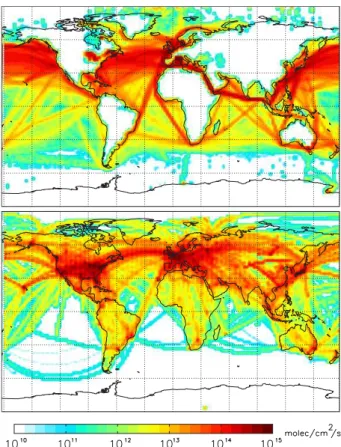
combustion associated with a reduction in international trade (Le Qu ´er ´e et al., 2009). For ship emissions related to international bunker fuel consumption, there is no sig-nificant duplication of emission with the main fossil fuel source in the model. Some shipping, especially close to shorelines could be from domestic trade, but this likely amounts to less than 15% (Endresen et al., 2003). Figure 3 shows the annual CO₂ 15

emissions in the model from shipping on a log scale for 2006, which clearly exhibits higher emissions over the oceans of the NH.

Emissions from aviation have been included in the GEOS-Chem sulfate simulation based on a 3-D distribution of emissions from the Atmospheric Effects of Aviation Project (AEAP) (Friedl, 1997). More recent studies by the System for Assessing Avia-20

tion Emissions (SAGE) (Kim et al., 2005, 2007) have continued to analyze the impact of aviation emissions. According to the SAGE assessment, the mean vertical profile of global aviation emissions has a small peak in the lowest kilometer (where takeo_ffand landing occur), is uniformly low between 1–9 km, and has a large peak from 9–12 km, with essentially no emissions above 12 km. Aviation emissions are most intense over 25

(15)

GMDD

3, 889–948, 2010

R. Nassar et al.

Title Page

Tables Figures

◭ ◮

Back Close

Full Screen / Esc

Discussion

P

a

per

|

Dis

cussion

P

a

per

|

Discussion

P

a

per

|

Discussio

n

P

a

per

to 154 Tg C in 1995. Kim et al. (2007) show a continued rise from 156 to 175 Tg C from 2000 to 2005, although Wilkerson et al. (2010) show a slight decline in 2006 at 162 Tg C. Figure 3 shows the annual column-integrated CO₂ emissions from aviation in GEOS-Chem for 2006, on a log scale.

Kim et al. (2005) partition the aviation fuel consumption (proportional to CO₂ emis-5

sions) into domestic and international components for eight regions of the world (roughly corresponding to the continents) for 2000–2004. Unlike international bunker fuels, domestic aviation fuel consumption is already included in national fossil fuel statistics and hence CO₂ inventories. Mean domestic aviation CO₂ emissions for 2000–2004, show that the North America region (which includes Central America and 10

the Caribbean) has the highest level of domestic aviation CO₂emitted (49.6 Tg C/yr), followed by Asia (16.1 Tg C/yr, excluding Russia and the Middle East) and Eastern Eu-rope (12.3 Tg C/yr). The other regions combined account for a mean of 9.8 Tg C/yr. To avoid “double-counting” the CO₂ emissions from domestic aviation in both the avi-ation and our main fossil fuel source, we subtract them from the main fossil fuel in-15

ventory in the following way. Annual sums of national fossil fuel use for each of the eight regions are determined. By subtracting the regional domestic aviation CO₂ from this sum a new corrected sum is found, which is used to determine a scale factor for each region in each year. This scale factor (which is close to unity) is then applied to the fossil fuel emissions for each region so that the seasonality and the distribution 20

within a region from the inventory are not changed, but CO₂ is conserved. With this approach, we maintain consistency with the assumed bunker fuel totals. For exam-ple in 2006, 189 Tg C came from international shipping and 65 Tg C from international aviation, within a fraction of a percent from the 255 Tg C emissions attributed to inter-national bunker fuel.

25

(16)

GMDD

3, 889–948, 2010

R. Nassar et al.

Title Page

Tables Figures

◭ ◮

Back Close

Full Screen / Esc

Discussion

P

a

per

|

Dis

cussion

P

a

per

|

Discussion

P

a

per

|

Discussio

n

P

a

per

|

2007). This altitude is also close to the height of peak sensitivity for CO₂retrieved from the thermal infrared satellite instruments AIRS (Chahine et al., 2005, 2008) and IASI (Crevoisier et al., 2009). In the first month shown in Fig. 4, the effects of shipping and aviation emissions are mainly local, with changes at the surface including both regions of increased CO₂from the additional emissions and decreased CO₂where the surface 5

correction has been applied to avoid double-counting of domestic aviation emissions. Over time, the CO₂ perturbation spreads vertically and zonally, then mixes throughout the NH before it is transported to the Southern Hemisphere (SH). After 3 years there is a persistent latitudinal gradient in the perturbation along with regions of nearly no increase where the adjustments to the land fossil fuel emissions were largest. The 10

e_ffect on the latitudinal gradient will be discussed quantitatively in Sect. 2.7.2.

2.7 Chemical production of CO₂from the oxidation of atmospheric carbon species

2.7.1 Background and method

Carbon monoxide (CO), methane (CH₄) and non-methane volatile organic carbons 15

(NMVOCs) are oxidized in the troposphere to produce CO₂but very few attempts have been made to account for this chemical source in global CO₂ transport models or in-verse modeling analyses. Early work on the subject was carried out first by Enting and Mansbridge (1991) with a 2-D model and later by Enting et al. (1995) with a 3-D model. This was followed by Baker (2001), Folberth et al. (2005) and Suntharalingam 20

et al. (2005), while Ciais et al. (2008) considered the importance of the chemical con-tribution to carbon balance of Europe. Chapter 7 of the Intergovernmental Panel on Climate Change (IPCC) Fourth Assessment Report (AR4, Denman et al., 2007) states the need for including the contribution from reduced carbon species in the total car-bon budget or for the comparison of inversions with bottom-up estimates, but most 25

(17)

GMDD

3, 889–948, 2010

R. Nassar et al.

Title Page

Tables Figures

◭ ◮

Back Close

Full Screen / Esc

Discussion

P

a

per

|

Dis

cussion

P

a

per

|

Discussion

P

a

per

|

Discussio

n

P

a

per

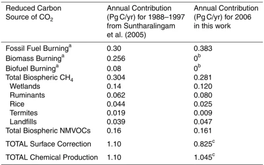
Fossil fuel emission inventories, such as from CDIAC, are based on CO₂ emis-sion factors that include direct emisemis-sions of CO₂ from fossil fuels as well as the CO₂ that chemically forms elsewhere in the atmosphere from the emission of other carbon species (Marland and Rotty, 1984). Use of these inventories in a model results in the CO₂ contribution from oxidation occurring directly at the surface rather than at a later 5

time at some distant location in the atmosphere after considerable transport. Sunthar-alingam et al. (2005) quantified this error with model simulations using CO₂ produc-tion from oxidaproduc-tion distributed throughout the atmosphere and an appropriate quantity subtracted from the surface emissions based on the spatial distributions of precursor emissions from fossil fuels, biomass and biofuel burning, wetlands, ruminants, rice, 10

termites and landfills, yielding a total of 1.10 Pg C/yr. The Suntharalingam et al. (2005) results have been directly applied offline by Jacobson et al. (2007b) in a joint global atmosphere-ocean inversion.

CO oxidation accounts for about 94% of the chemical production of CO₂ (Folberth et al., 2005) because CO is an intermediate for the oxidation of CH₄ and NMVOCs 15

to CO₂ and CO₂is the only significant product from CO oxidation. Therefore, we use the GEOS-Chem NO_x-O_x-hydrocarbon simulation to obtain monthly CO loss rates for the period 2004–2009 inclusive. These CO loss rates are essentially equal to the CO₂ production rates and are used in the model as a 3-D source inventory for the chemical production of CO₂.

20

Accounting for the surface correction requires accounting for emissions of all reac-tants that undergo oxidation to CO₂that were already included in emission inventories, then appropriately subtracting that quantity. The surface correction discussed above is not necessary for inventories like GFED or the biofuel inventory, which explicitly ac-count for CO₂, CO, CH₄and NMVOC emissions using the emission factors of Andreae 25

(18)

GMDD

3, 889–948, 2010

R. Nassar et al.

Title Page

Tables Figures

◭ ◮

Back Close

Full Screen / Esc

Discussion

P

a

per

|

Dis

cussion

P

a

per

|

Discussion

P

a

per

|

Discussio

n

P

a

per

|

4.89% of national emissions for 1988–1997, so we assume this constant percentage for contemporary values and proportionally scale down the spatially-distributed CDIAC emissions, assuming no regional variability in combustion completeness, although de-veloped countries typically have stricter pollution controls and may have more complete combustion resulting in lower levels of CO, CH₄and NMVOC emissions thus requiring 5

a smaller correction factor.

Randerson et al. (2002) discuss the need for clarity in the definition of Net Ecosys-tem Production (NEP) and other quantities that are sometimes stated in terms of CO₂ and other times in terms of total carbon. Since they advocated for a definition including all carbon fluxes, non-CO₂carbon emissions from CASA NEP (Olsen and Randerson, 10

2004) must be accounted for through a surface correction. To account for CH₄ from the biosphere we take the CH₄source distribution from a GEOS-Chem CH₄simulation for 2004, which includes monthly averaged emissions from wetlands (bogs, swamps, tundra, etc.) and annually averaged emissions from livestock, landfills/waste, rice pro-duction and other natural sources (mainly termites). The combined annual sum of all 15

biogenic methane sources is shown in Fig. 5 with the breakdown in Table 1. As in Duncan et al. (2007) and Suntharalingam et al. (2005), we assume a CH₄to CO₂ con-version e_fficiency of unity. Other biogenics are accounted for using the spatial distribu-tion of isoprene and monoterpenes from a 2004 GEOS-Chem simuladistribu-tion that was run using emission factors from the MEGAN inventory (Guenther et al., 2006, 2007). This 20

yielded annual biospheric emissions of 351 Tg C of isoprene and 132 Tg C of monoter-penes. Figure 5 shows that the most intense biospheric emissions of isoprene and monoterpenes came from the Amazon, Equatorial Africa, Indonesia and the South-Eastern United States. Unlike methane, the conversion e_fficiency of these species to CO is only about 0.20 (Duncan et al., 2007) but we instead apply a conversion factor 25

(19)

GMDD

3, 889–948, 2010

R. Nassar et al.

Title Page

Tables Figures

◭ ◮

Back Close

Full Screen / Esc

Discussion

P

a

per

|

Dis

cussion

P

a

per

|

Discussion

P

a

per

|

Discussio

n

P

a

per

Suntharalingam et al. (2005). Our surface corrections are smaller than those of Sun-tharalingam et al. (2005) and not balanced with our CO₂chemical production, since we have not adjusted surface emissions for chemical production related to biomass and biofuel burning inventories since they already use separate emission factors for each individual species (van der Werf et al., 2006; Yevich and Logan, 2003; Andreae and 5

Merlet, 2001).

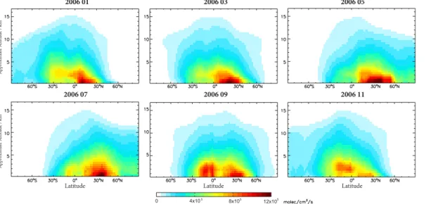
Figure 6 displays the vertical, latitudinal and monthly variability in CO₂chemical pro-duction for selected months in 2006. Peak propro-duction typically occurs from the surface to about 4 km in the NH tropics, however in September to November 2006, intense CO₂production occurred in the SH, likely related to Indonesian biomass burning. This 10

can be confirmed by the spatial patterns in Fig. 7, which shows the monthly chemical production of CO₂ at model level 22, near 5 km altitude. This altitude was selected for comparison since it is the altitude of peak sensitivity for CO₂ measurements by the Tropospheric Emission Spectrometer (TES) (Kulawik et al., 2009), which are be-ginning to be used for assimilation with GEOS-Chem CO₂ simulations (Nassar et al., 15

2010). In both Figs. 6 and 7, chemical production of CO₂exhibits clear local, latitudi-nal and seasolatitudi-nal variability which should impact inverse modeling. The most intense chemical production is mainly localized over China but is occasionally seen in other regions, most likely related to biomass burning, such as over Siberia in July, Indonesia from August to November and Southern Australia in December (not shown). Although 20

the CO₂ chemical production is mainly bounded by 60◦_S–60◦_{N, significant CO}

2 pro-duction is observed in the Arctic and the Antarctic during their respective summers. Interestingly, no biomass burning signature is seen over the Amazon, which is a local minimum in CO₂ production for most months at this level, thus indicating that con-version of CO to CO₂ is dependent on multiple chemical and dynamical factors and 25

(20)

GMDD

3, 889–948, 2010

R. Nassar et al.

Title Page

Tables Figures

◭ ◮

Back Close

Full Screen / Esc

Discussion

P

a

per

|

Dis

cussion

P

a

per

|

Discussion

P

a

per

|

Discussio

n

P

a

per

|

have a significant impact when applying the model simulation to inverse modeling of terrestrial surface fluxes.

2.7.2 Impact of the chemical pump on atmospheric CO₂

The impact of the chemical pump is shown in Fig. 8 at the surface and at the model level near 5 km, for time intervals of up to 3 years. After one month, we see locally de-5

creased CO₂ at the surface in the NH, with almost no e_ffects at 5 km. After 3 months, we see regions of decreased CO₂ in the NH and increased CO₂in the SH at the sur-face, with the same pattern at 5 km albeit somewhat weaker. Although a negative per-turbation from the chemical source persists at the surface from 6 months to 3 years, at 5 km altitude the perturbation is positive globally beyond about 6 months with a strong 10

latitudinal gradient. After 3 full years the perturbation at 5 km slightly exceeds the per-turbation at the surface for high southern latitudes. The zonally-averaged impacts of the chemical source and emissions from shipping and aviation are shown in Fig. 9 for both the surface and the model level nearest to 5 km. This indicates a decrease of

∼0.25 ppm in the gradient between Mauna Loa (19.54◦_{N) and the South Pole after one} 15

year as a result of the chemical source. After 4 complete years, the zonal impact of the chemical source in the SH is∼0.60 ppm while for NH midlatitudes it ranges from ∼0.15–0.25 ppm. The zonal impact from shipping and aviation in Fig. 9, partially o_ff -sets the impact of the chemical source on the latitudinal gradient. By the end of the fourth year, the combined impact of shipping and aviation emissions with CO₂ chemi-20

cal production is∼1.0 ppm in the SH, and somewhat less in the NH with a minimum of

∼0.70 ppm around 40–50◦N. It should be noted that the simulation maintains a

persis-tent change in gradient even after much inter-hemispheric mixing has occurred. While shipping and aviation increase the global CO₂latitudinal gradient by just over 0.1 ppm, the inclusion of CO₂ chemical production (and the surface correction) decreases the 25

(21)

GMDD

3, 889–948, 2010

R. Nassar et al.

Title Page

Tables Figures

◭ ◮

Back Close

Full Screen / Esc

Discussion

P

a

per

|

Dis

cussion

P

a

per

|

Discussion

P

a

per

|

Discussio

n

P

a

per

The global offset in CO₂ mixing ratios which results from inclusion of the chemi-cal source specifichemi-cally relates to the additional CO₂ in the model system due to the imbalance between the chemical source and the surface correction (Table 1), associ-ated with reduced carbon emissions from biomass and biofuel combustion. We do not correct for them here as our surface emissions from biomass burning and biofuel com-5

bustion (derived from GFED and Yevich and Logan, 2003) include only direct emissions of CO₂.

2.7.3 Assimilated CO for determination of CO2production rates

A major limitation in using the O_x-NO_x-hydrocarbon model simulation to estimate the chemical source of CO₂ is that bottom-up CO inventories are highly uncertain. For 10

example, Kopacz et al. (2010) conducted an inversion analysis of CO observations from four di_fferent satellite instruments and found that the CO emission inventory in GEOS-Chem significantly underestimated wintertime CO emission. Inferred emissions from North America and Europe were 50% larger in winter than the specified bottom-up emissions in the model, whereas inferred emission estimates from Asia were 100% 15

greater in winter. Kopacz et al. (2010) attributed this discrepancy to an underestimate of emissions from vehicle cold starts and residential heating in the bottom-up inventory. These biases in the bottom-up inventory will result in an underestimate of the CO₂ pro-duction rate calculated from the model. An alternative approach is to assimilate obser-vations of atmospheric CO to obtain an improved description of the CO distribution in 20

the model and, thus, a more accurate estimate of CO₂production rates.

Parrington et al. (2008) used a sequential sub-optimal Kalman filter to assimilate TES observations of ozone and CO into the GEOS-Chem O_x-NO_x-hydrocarbon simulation. We have extended the Parrington et al. (2008) study to assimilate TES CO data for 2006 into the current version of GEOS-Chem. We focus on 2006 for the assimilation 25

(22)

GMDD

3, 889–948, 2010

R. Nassar et al.

Title Page

Tables Figures

◭ ◮

Back Close

Full Screen / Esc

Discussion

P

a

per

|

Dis

cussion

P

a

per

|

Discussion

P

a

per

|

Discussio

n

P

a

per

|

assimilation significantly increases the CO abundance in the model, consistent with the results of Kopacz et al. (2010). The right panels in Fig. 7 show the impact of basing our CO₂ production on assimilated TES CO observations for 2006. The CO₂ production rates are weakly enhanced between∼0–40◦N from January to March. In

January the globally averaged production rate is about 5% larger with the assimilation, 5

whereas in March it is 13% greater. There are small reductions in the CO₂ produc-tion rates over the Amazon and across the Atlantic to Southern Africa in January. The largest di_fferences in CO₂production rates are obtained between 0◦_–40◦_{N during May} to June, when the assimilation enhances the globally-averaged CO₂ production by as much as 24%. The assimilation results in an increase in the global annual CO₂ pro-10

duction rate from 1.045 Pg C/yr to 1.181 Pg C/yr. After a 1-year simulation (2006), the run with assimilated CO produced CO₂that was ∼0.08 ppm higher than our standard

chemical production run near 5 km over much of the NH and a localized perturbation of 0.85 ppm at this altitude over equatorial Africa. To our knowledge, this represents the first satellite-derived estimate of the chemical source of CO₂. We are exploring further 15

the use of the assimilation of TES CO data in our inversion analysis of the TES CO₂ data in Nassar et al. (2010).

3 GEOS-Chem CO₂simulations and comparisons

In this section, we will evaluate GEOS-Chem CO₂ simulations that have used the fluxes described in the previous section. The primary simulation was carried out using 20

GEOS-5 meteorological fields at 2◦latitude×2.5◦longitude resolution, with 47 vertical

hybrid-sigma levels up to 0.01 hPa. Since CO₂ has a long atmospheric lifetime, ini-tial concentrations strongly impact model results. The total global average CO₂ in the model atmosphere at the start of the run will have a much larger impact than specific features of the CO₂ distribution. For this work, we begin with a uniform global distri-25

(23)

GMDD

3, 889–948, 2010

R. Nassar et al.

Title Page

Tables Figures

◭ ◮

Back Close

Full Screen / Esc

Discussion

P

a

per

|

Dis

cussion

P

a

per

|

Discussion

P

a

per

|

Discussio

n

P

a

per

(http://www.esrl.noaa.gov/gmd/ccgg/trends/#global), the global marine surface annual mean CO₂in 2003 was 374.93 ppm, with monthly means of 376.31 ppm in December 2003 and 376.97 ppm in January 2004. The total tropospheric mean CO₂for 1 January 2004 is related to these values but also dependent on values over land which are highly variable but tend to be slightly higher than marine values in January, as well as the ver-5

tical profile of CO₂, which generally decreases with height in the NH and increases slightly with height in the SH. These facts make approximating mean tropospheric CO₂ di_fficult, but suggest that 375.0 ppm for 1 January 2004 is a reasonable starting point for a spin-up and subsequent simulation. In the following section, we examine model results from the aforementioned run.

10

3.1 Spatial and temporal comparisons with GLOBALVIEW-CO2

Figure 10 shows the annually averaged GEOS-Chem CO₂ concentration for 2006 at the surface and around 5 km, from a run with emissions from shipping, aviation, the chemical source and other fluxes. CO₂ values are generally higher in the NH with a gradual pole-to-pole gradient at both altitudes. This gradient is mainly a result of the 15

predominant emission of fossil fuels occurring in the NH and is roughly consistent with the expected gradient based on 2006 emission values (Taylor and Orr, 2000; Keeling et al., 2005), and is discussed more quantitatively later. The model level near 5 km clearly shows a smaller range of values than at the surface as well as a reduced distinction between CO₂ over land and ocean. Overall, the difference between minimum and 20

maximum values in annually-averaged surface CO₂ is only ∼25 ppm or ∼6%, which

is much smaller than those for tropospheric trace gases with shorter lifetimes such as CO, O₃(i.e. Nassar et al., 2009) or CH₄. It should be noted that this range is somewhat specific to a resolution of 2◦

×2.5◦_{and a finer resolution (or true point measurements)} would lead to a slightly larger range.

25

(24)

GMDD

3, 889–948, 2010

R. Nassar et al.

Title Page

Tables Figures

◭ ◮

Back Close

Full Screen / Esc

Discussion

P

a

per

|

Dis

cussion

P

a

per

|

Discussion

P

a

per

|

Discussio

n

P

a

per

|

simulation represents the north-south CO₂ gradient reasonably well, although some di_fferences are noticeable at high southern latitudes (less than 0.5 ppm) and will be discussed in detail later. Agreement at marine and coastal sites is better than that at inland sites (for example in Europe), which can be affected by strong inland sources and sinks.

5

Representation errors due to finite resolution are a serious limitation of current CO₂ models and complicate these comparisons, especially those at inland and coastal sites. Figure 11 illustrates this problem for Mauna Loa, by displaying the horizontal surface variability around Hawaii and the vertical profile of the Mauna Loa gridbox. Although we can have very accurate in situ point measurements or flask measurements, comparing 10

these to the model is a challenge because of representativeness. In the horizontal di-rection, the gridbox with which we compare is 222 km×261 km, encompassing the big

island of Hawaii, a portion of a smaller island (Maui) and much of the ocean. True hori-zontal variability in the CO₂mixing ratio, which the point measurement only samples, is averaged over the entire gridbox in the model, which can lead to an apparent discrep-15

ancy although both values could be accurate. Vertical representativeness errors are even more of a challenge. Mauna Loa measurements sample air at 3.4 km up the peak of the 4.2 km mountain, but because of the topography within this gridbox, the lowest model level spans 0–4.2 km altitude while a single surface pressure must be used in determining the model hybrid sigma level. The mean surface pressure of the gridbox 20

(25)

GMDD

3, 889–948, 2010

R. Nassar et al.

Title Page

Tables Figures

◭ ◮

Back Close

Full Screen / Esc

Discussion

P

a

per

|

Dis

cussion

P

a

per

|

Discussion

P

a

per

|

Discussio

n

P

a

per

To evaluate the model seasonal cycle, we make timeseries comparisons between point measurements at a number of GLOBALVIEW locations. In Fig. 12, timeseries comparisons are made between GLOBALVIEW and a multi-year simulation with ship-ping, aviation, the chemical source and other fluxes for the period 1 January 2004 to 31 December 2008. A 7-day moving average has been applied to the modeled data, while 5

the GLOBALVIEW consists of_∼7.6-day averages, with a 40-day low-pass filter applied to residuals (Masarie and Tans, 1995). More variability is evident in the model time-series than the GLOBALVIEW timetime-series, which appears smoother as a result of the low-pass filtering. We do not apply the same filtering approach to our data since this variability on short time scales in the model could be of interest for certain applications, 10

but should theoretically average out over time.

Aside from the fine scale features of the model CO₂ timeseries, the model rep-resents the seasonal variability at each station reasonably well. The characteristic near-sinusoidal seasonal cycle is largest in the mid- to high latitudes of the NH over land (such as Fraserdale) consistent with NH vegetation absorbing CO₂ in the boreal 15

growing season and the release of CO₂ by vegetation at the end of the growing sea-son (Keeling, 1960). This pattern is predominantly driven by terrestrial fluxes from CASA, while much smaller contributions to the seasonal cycle include fossil fuel burn-ing, biomass burnburn-ing, ocean exchange and the chemical source. (The magnitude of the seasonal impact from fossil fuel emissions is quantified and discussed earlier.) The 20

seasonal cycle amplitude typically decreases moving southward, since the SH has less midlatitude vegetation to seasonally absorb and release CO₂. The least seasonal variability is evident at Antarctic locations and in particular the South Pole, farthest from sources and sinks. There are a few unexplained exceptions to this generally good agreement, the worst one being the Indonesia station Bukit Kototabang (0.20◦_S, 25

(26)

GMDD

3, 889–948, 2010

R. Nassar et al.

Title Page

Tables Figures

◭ ◮

Back Close

Full Screen / Esc

Discussion

P

a

per

|

Dis

cussion

P

a

per

|

Discussion

P

a

per

|

Discussio

n

P

a

per

|

Since the initialization of the model run began on 1 January 2004 with a uniform CO₂ distribution, the start of the timeseries show low biases at NH high latitudes (Alert, Summit, Barrow, etc.) and smaller low biases at SH high latitudes (South Pole, Cape Grim, Macquarie Island, etc.). For Mauna Loa, much of the tropics and many SH stations, the uniform global value is already a close approximation. After less than 6 5

months of the model spin-up, realistic features develop including better agreement at the higher latitudes as a result of the various drivers of the rectifier effect.

The free-running model exhibits a slight high drift over time, with most of the depar-ture from GLOBALVIEW mainly becoming evident in 2007. Some drift as observed here is expected since we are running with an annual terrestrial exchange (based on 10

the 1991–2000 period) and ocean exchange that are not increasing in conjunction with increasing fossil fuel CO₂emissions. A strong body of evidence indicates that as emis-sions increase, Earth’s natural sinks are taking up greater amounts of CO₂since only very subtle trends are currently observed in the airborne fraction (Gloor et al., 2010). This drift is not a problem for use of the model simulations in the context of data assim-15

ilation or inverse modeling, since observational data will constrain the drift or minimize the error in a posteriori fluxes as necessary.

Figure 13 illustrates the latitudinal gradient obtained from our simulations with and without the chemical source. Here we see that the chemical source gives persistently better agreement with GLOBALVIEW-CO₂in the SH, where the run without the chem-20

ical source is persistently lower than GLOBALVIEW-CO₂. For the NH, the run with the chemical source is superior for two out of three years, but is positively biased in 2007. Since the CO₂ chemical source is indeed a real contributor to atmospheric CO₂, the fact that the drift is greater when it is included highlights the fact that sinks such as annual terrestrial uptake are likely increasing at an even greater rate than we might 25

(27)

GMDD

3, 889–948, 2010

R. Nassar et al.

Title Page

Tables Figures

◭ ◮

Back Close

Full Screen / Esc

Discussion

P

a

per

|

Dis

cussion

P

a

per

|

Discussion

P

a

per

|

Discussio

n

P

a

per

CDIAC.

We note that the lines and symbols in Fig. 13 are not expected to coincide since the symbols are point or single pixel measurements, while the lines are zonal averages. Figure 13 highlights the reduced latitudinal gradient at a higher altitude in the model (also shown in Fig. 10), in which there is actually higher annually-averaged CO₂ at 5

5 km than at the surface south of ∼20◦S. The pole-to-pole CO2 differences can be closely approximated by the Alert (82.45◦N) to South Pole (90◦S) differences which are summarized in Table 3, along with Mauna Loa (19.5◦_{N) to South Pole di}

fferences. While the run without the chemical source persistently overestimates both the Mauna Loa and Alert offsets, the chemical source has some higher offsets and occasional 10

lower o_ffsets, with consistently better o_ffsets at Mauna Loa. This highlights the fact that although both simulations drift to high CO₂in the NH, skewing the latitudinal gradient, the problem is somewhat reduced with the chemical source.

3.2 Vertical profile comparisons

The GLOBALVIEW-CO₂data set contains some limited measurements of the vertical 15

structure of CO₂ based on in situ or flask measurements from aircraft at select loca-tions. Figure 14 shows comparisons of monthly-averaged GEOS-Chem profiles with GLOBALVIEW at a NH coastal site (Estevan Point, BC, Canada), a NH continental site (Park Falls, WI, USA) and a SH remote island site (Rarotonga, Cook Islands, South Pacific Ocean) for 2006. At Estevan Point, the shape and slope of the vertical profile 20

agree very well for most months. In May and June, GLOBALVIEW indicates slightly lower values at the lowest level (0.5 km) than at higher levels (1.5–5.5 km), a feature not present in our model at this location and time but does appear in July–September, when GLOBALVIEW values at 0.5 km have increased. The physical reason for this two-month lag in the model is not known, but it could relate to either CASA or the two-monthly 25

ocean flux variability, neither of which correspond to an El Ni ˜no year like 2006.