BGD
5, 3699–3736, 2008GHG emissions from alpine reservoirs
T. Diem et al.
Title Page
Abstract Introduction
Conclusions References
Tables Figures
◭ ◮
◭ ◮
Back Close
Full Screen / Esc
Printer-friendly Version
Interactive Discussion
Biogeosciences Discuss., 5, 3699–3736, 2008 www.biogeosciences-discuss.net/5/3699/2008/ © Author(s) 2008. This work is distributed under the Creative Commons Attribution 3.0 License.
Biogeosciences Discussions
Biogeosciences Discussionsis the access reviewed discussion forum ofBiogeosciences
Greenhouse gas emissions
(CO
2
, CH
4
and N
2
O) from perialpine and
alpine hydropower reservoirs
T. Diem, S. Koch, S. Schwarzenbach, B. Wehrli, and C. J. Schubert
Department of Surface Waters, EAWAG, Kastanienbaum, Switzerland
Received: 11 August 2008 – Accepted: 18 August 2008 – Published: 10 September 2008
Correspondence to: T. Diem ([email protected])
BGD
5, 3699–3736, 2008GHG emissions from alpine reservoirs
T. Diem et al.
Title Page
Abstract Introduction
Conclusions References
Tables Figures
◭ ◮
◭ ◮
Back Close
Full Screen / Esc
Printer-friendly Version
Interactive Discussion
Abstract
In eleven reservoirs located at different altitudes in Switzerland depth profiles of green-house gas (CO2, CH4, and N2O) concentrations were measured several times during spring and summer. Trace gas emissions were calculated using surface concentra-tions, wind speeds and transfer velocities. Additionally we assessed methane loss at
5
the turbine and the methane input by inflowing water. All reservoirs were net emit-ters of CO2with an average of 1030±780 mg m−2d−1and of methane with an average
of 0.20±0.15 mg m−2d−1. One reservoir (Lake Wohlen) emitted methane at a much
higher rate (160±110 mg m−2d−1), most of which (>98%) was due to ebullition. Only
lowland reservoirs were sources for N2O (72±22µg m− 2
d−1), while the subalpine and
10
alpine reservoirs seem to be in equilibrium with atmospheric concentrations. Methane loss at the turbine was as large as the diffusive flux from the surface for two subalpine reservoirs and around five times smaller for a lowland reservoir. The available data suggests greenhouse gas emissions from reservoirs in the Alps are minor contributors to the global greenhouse gas emissions.
15
1 Introduction
In the early 1990s artificial lakes and reservoirs were discovered as potential green-house gas emitters (Kelly et al., 1994; Rudd et al., 1993). The question was put for-ward, whether hydroelectric reservoirs, especially in the tropics could still be consid-ered cleaner energy sources, compared to fossil alternatives (Fearnside, 1997, 2002).
20
There is however, a high variety of trace gas emissions between different reservoirs, which leads to large uncertainties in the quantification of global emissions. Another problem is the small number of available data. Several studies were done in tropi-cal (e.g. Galy-Lacaux et al., 1997, 1999; Keller and Stallard, 1994; Rosa et al., 2003, 2004) and boreal reservoirs (e.g. Duchemin et al., 1995; Rudd et al., 1993; Tremblay
25
BGD
5, 3699–3736, 2008GHG emissions from alpine reservoirs
T. Diem et al.
Title Page
Abstract Introduction
Conclusions References
Tables Figures
◭ ◮
◭ ◮
Back Close
Full Screen / Esc
Printer-friendly Version
Interactive Discussion
in the temperate climate zone (Soumis et al., 2004). Both in the tropics and in bo-real/temperate reservoirs CO2 is the most emitted trace gas (St. Louis et al., 2000). Taking the Global Warming Potential (GWP) into account, methane release in the trop-ics contributes more to global warming than CO2 since the GWP of CH4 is 25 times that of CO2on a 100 year basis (Forster et al., 2007).
5
In this study we try to increase the knowledge of greenhouse gas emissions from hydropower reservoirs across an altitude gradient in the Alps, Central Europe. We calculated diffusive fluxes of CO2, CH4 and N2O from the surface concentrations of several Swiss reservoirs at different times of the year. Eleven reservoirs at different altitudes allowed a comparison of greenhouse gas emissions under different climatic
10
conditions and possible changes in the importance of CO2compared to CH4release. Nitrous oxide emissions from freshwater bodies published so far are very small and often linked to the littoral zones of the lakes (Huttunen et al., 2003; Wang et al., 2007). N2O production in lakes is not limited by low temperatures, as Huttunen et al. (2002) reported N2O accumulation during winter in two boreal reservoirs. Swiss alpine
reser-15
voirs have little or no littoral zones, as the water depth increases very fast along the steep mountain slopes and the reservoirs are usually deeper than 50 m. By measuring N2O concentrations in reservoirs at different elevations the relevance of littoral zones for N2O production in cold water reservoirs and consequently N2O emissions is inves-tigated.
20
Besides methane supersaturation in lakes and reservoirs, enhanced methane con-centrations have been found in rivers (Abril et al., 2006; de Angelis and Lilley, 1987) and below the outlet of reservoirs (Kemenes et al., 2007). The importance of these addi-tional sources and sinks of methane in hydropower reservoirs is assessed by methane concentration and carbon isotopic composition measurements. The isotopic
compo-25
BGD
5, 3699–3736, 2008GHG emissions from alpine reservoirs
T. Diem et al.
Title Page
Abstract Introduction
Conclusions References
Tables Figures
◭ ◮
◭ ◮
Back Close
Full Screen / Esc
Printer-friendly Version
Interactive Discussion
increase inδ13C (Barker and Fritz, 1981; Whiticar, 1999). Turbulent diffusion does not affect the isotopic composition of methane and the change caused by methane emis-sion is small (Knox et al., 1992). The use of carbon isotopic composition also helps to distinguish between internal and external methane sources in the reservoirs
2 Study sites
5
From September 2003 to August 2006 eleven Swiss reservoirs from different areas and elevations were sampled for greenhouse gases (Table 1 and Fig. 1). The reservoirs are distributed along an elevation gradient from 481 to 2368 m a.s.l. Hence, climate varies greatly between the different reservoirs. Average yearly temperatures range from about 8◦C at Lake Wohlen to nearly 0◦C at Lake Oberaar. Precipitation in the reservoirs of
10
the central part of Switzerland is up to four times higher than for the reservoirs in the southwestern parts and eastern parts of the country.
Electricity production for most Swiss storage reservoirs is higher in winter than in summer, while the majority of the water filling the reservoirs is available from spring to autumn. This leads to a large decline in reservoir water level. In some cases the
15
remaining water in early spring is less than 10% of the maximum water volume. Two of the reservoirs (Lakes Oberaar and Sihl) are pump-storage reservoirs, which receive water from a lower lying reservoir (Lake Grimsel for Lake Oberaar) or lake (Lake Zurich for Lake Sihl). While the water volume of Lake Oberaar gets replaced up to 10 times every year, pumping only contributes a minor part to Lake Sihl.
20
Seven of the reservoirs (Lake Wohlen, Lake Gruy `ere, Lake Sihl, Lake Luzzone, Lake Santa Maria, Lake Oberaar and Lake Lungern) were sampled several times during the campaign to investigate changes in the temporal development of the greenhouse-gas concentrations. The first six reservoirs were sampled three times from May 2005 to August 2005. Due to snow conditions, measurements at higher elevations started later
25
BGD
5, 3699–3736, 2008GHG emissions from alpine reservoirs
T. Diem et al.
Title Page
Abstract Introduction
Conclusions References
Tables Figures
◭ ◮
◭ ◮
Back Close
Full Screen / Esc
Printer-friendly Version
Interactive Discussion
3 Methods
3.1 Hydrographic data
A SBE 19 CTD probe (Sea Bird Electronics) equipped with oxygen and pH sensors was used to collect hydrographic data (conductivity, temperature, depth, light trans-mission, pH and dissolved oxygen). The water column was sampled with a 5l Niskin
5
bottle and aliquots were immediately transferred into sample bottles with plastic tubing (Winkler bottles for oxygen, 600 ml glass bottles for methane and nitrous oxide concen-tration and 200 ml plastic bottles for alkalinity). Winkler samples were used to correct the offset in the oxygen sensor. Alkalinity was titrated with 0.1 M HCl. Samples for dis-solved gas analysis were flushed with 2–4 times the bottle volume before the samples
10
were preserved with NaOH (pH>12) or Cu(I)Cl, closed with butyl septa, while carefully avoiding air bubbles in the bottles. To calibrate the pH sensor, solutions of known pH (pH=4, 7 and 9) were used before each sampling date.
3.2 Dissolved gases
3.2.1 CO2
15
Dissolved CO2was calculated using the measured alkalinity, temperature, pH, and the dissociation constants of H2CO3 and HCO−3 (Plummer and Busenberg, 1982). Sam-ples for alkalinity were only taken at the surface and at the bottom of the water column. According to Neal et al. (1998) the error of CO2 concentration calculations using temperature and pH is less than 2% for pH values<9. The error of pH measurement
20
BGD
5, 3699–3736, 2008GHG emissions from alpine reservoirs
T. Diem et al.
Title Page
Abstract Introduction
Conclusions References
Tables Figures
◭ ◮
◭ ◮
Back Close
Full Screen / Esc
Printer-friendly Version
Interactive Discussion
3.2.2 CH4and N2O
Concentrations of dissolved methane and nitrous oxide were measured by the headspace technique similar to McAuliffe (1971). A sample volume of 50 ml was re-placed by an inert gas (helium or nitrogen) and equilibrated in an ultra-sonic bath for about 30 min. Nitrous oxide was measured with a Dani 86.10 HT gas chromatograph
5
(GC) with a Porapak Q column (Supelco) and an electron capture detector (ECD). The oven temperature was kept constant at 70◦C and the detector temperature was 340◦C. Methane concentrations were measured on a HRGC 5160 Mega Series (Carlos Erba Instruments) with a flame ionization detector (FID), a GS-Q P/N 115-3432 column (J and W Scientific) and hydrogen as a carrier gas. Temperatures were 40◦C for the
10
oven and 200◦C for the detector. Gas volumes of 2 ml for N2O and 200µl for CH4were injected. Replicate measurements yielded an accuracy of±5% for methane and±10%
for nitrous oxide.
From 2006 on, the measurements were made on an Agilent GC using a GS-Carbonplot column (Agilent) for nitrous oxide and a Carboxen 1010 Plot column
(Su-15
pelco) for methane. Again an ECD was used for N2O and a FID for CH4. The temper-ature was kept constant at 40◦C for 5 minutes and then raised to 120◦C at the rate of 10◦C/min. The GC had a 1-ml sample loop for nitrous oxide and a 500µl sample loop for methane. Accuracy on this GC improved to±3% for methane and±5% for nitrous
oxide.
20
Standards used for calibration were supplied from Scotty Specialty Gases. Concen-trations were 15 ppm, 1000 ppm and 1% for methane and 1 ppm and 10 ppm for nitrous oxide.
Dissolved gas concentrations were calculated using solubility data from Wiesenburg and Guinasso (1979) for methane, from Weiss and Price (1980) for nitrous oxide and
25
BGD
5, 3699–3736, 2008GHG emissions from alpine reservoirs
T. Diem et al.
Title Page
Abstract Introduction
Conclusions References
Tables Figures
◭ ◮
◭ ◮
Back Close
Full Screen / Esc
Printer-friendly Version
Interactive Discussion
3.3 Stable isotopes
The isotopic signature of methane was determined similar to the method described by (Sansone et al., 1997). Measurements were done with an IsoPrime mass spectrom-eter connected to a TraceGas preconcentrator (GV Instruments, UK). The amount of injected gas depended on the sample concentration, ranging from a fewµl to several
5
ml. Results are noted in the standardδ-notation relative to Vienna PeeDee Belemnite (VPDB).
δ13C
=( Rsample RReference
−1)×1000 (1)
HereRsampleis the ratio of 13
C/12C of the sample andRreferencethe ratio of the reference material andδ13C the isotopic signature of methane in ‰ vs. VPDB. A Standard (1%
10
CH4in argon) of known isotopic composition was injected between every two or three sample runs. The accuracy of the method was±0.7 ‰.
3.4 Gas fluxes
Greenhouse-gas fluxes were calculated using the boundary layer model as described by Liss and Slater (1974).
15
F=k·c·(Cw−Ceq) (2)
The model estimates the air-water flux F [mg m−2d−1] using the water saturation con-centration Ceq [M], the measured water concentration Cw [M] of the greenhouse-gas, the transfer velocity k [cm h−1] and a unit conversion factor c. For the calculation of the transfer velocity k we used the bi-linear relationship given by (Crusius and Wanninkhof,
20
2003):
BGD
5, 3699–3736, 2008GHG emissions from alpine reservoirs
T. Diem et al.
Title Page
Abstract Introduction
Conclusions References
Tables Figures
◭ ◮
◭ ◮
Back Close
Full Screen / Esc
Printer-friendly Version
Interactive Discussion
forU10>3.7 m s−1 k600=4.33U10−13.3
wherek600 is the transfer velocity for the Schmidt number Sc=600, andU10 the wind speed ten metres above the ground. To convert k600 to the actual transfer velocity k of the gas we used
5
k=k600(Sc/600)c (3)
whereScis the Schmidt number of the greenhouse gas (CH4, CO2and N2O) at water surface temperature andcis−2/3 forU10<3.7 m s−
1
and−1/2 for higher wind speeds
(Liss and Merlivat, 1986).
Equilibrium concentrations were determined using an air concentration of 1.77 ppm
10
CH4, 379 ppm CO2 and 319 ppb N2O (Forster et al. 2007), corrected to the reduced pressure of the lake elevation, and measured water temperatures. Schmidt numbers were calculated for the measured water temperatures according to Wanninkhof (1992) and the authors cited therein. Wind data was supplied by MeteoSwiss from the ANETZ-or ENET-Station closest to the lake in question.
15
3.5 Methane mass balance studies
Several of the following methods were used to allow a simple mass balance of methane fluxes in and out of the reservoirs. Table 1 gives an overview what measurements were done in which reservoirs.
3.5.1 Sediment cores
20
Cores were taken with a gravity corer. Samples were collected every centimetre from holes in the side of the core using a plastic syringe. 2 ml of sediment and 5 ml of NaOH (5%) were filled into 25 ml glass bottles and closed with butyl septa. Methane concentration and isotopic composition were measured in the headspace as described above.
BGD
5, 3699–3736, 2008GHG emissions from alpine reservoirs
T. Diem et al.
Title Page
Abstract Introduction
Conclusions References
Tables Figures
◭ ◮
◭ ◮
Back Close
Full Screen / Esc
Printer-friendly Version
Interactive Discussion
3.5.2 Ebullition
To estimate methane flux from the sediments via bubbles, funnels were deployed around one meter above the sediment and left for several hours in one spot. Gas bubbles were sampled in a cylinder on top of the funnel. The volume of gas was esti-mated from the area of the cylinder no longer filled with water. Samples were collected
5
from the cylinder through a butyl septum and filled into pre-evacuated, sealed 25 ml glass bottles. These bottles were taken to the lab and analyzed for concentrations and isotopic signature as described above.
3.5.3 Inflows, outflows
Methane flowing in and out of the reservoirs was sampled in six reservoirs. If possible
10
the CTD probe was used, but if depth of the river was not sufficient, temperature and conductivity were measured with a WTW LF 330 conductivity meter, pH with a Metrohm 704 pH-meter and oxygen with a WTW Multi 340i multi probe. Samples for methane measurements were sampled as described above. Only major inflows were sampled, as well as spill-water from the reservoir and water after passage of the turbine.
15
4 Results
4.1 CO2concentrations and emissions
Surface concentrations of CO2were supersaturated in all five reservoirs for which data are available (Table 2), with concentrations ranging from 40–280µM. This is in ac-cordance with findings by Cole et al. (1994), who analyzed lakes world-wide, most of
20
BGD
5, 3699–3736, 2008GHG emissions from alpine reservoirs
T. Diem et al.
Title Page
Abstract Introduction
Conclusions References
Tables Figures
◭ ◮
◭ ◮
Back Close
Full Screen / Esc
Printer-friendly Version
Interactive Discussion
The fluxes we calculated were on average 1030±780 mg m−2d−1 (Median
710 mg m−2d−1). Emissions at the first sampling dates in May are nearly four times higher (1820±490 mg m−2d−1) than at the remaining dates (520±290 mg m−2d−1;
Ta-ble 2).
In low conductivity lakes we had a problem with the pH sensor we used. The
accu-5
racy of the sensor was not sufficient for these conditions and concentrations and fluxes for reservoirs with conductivities below 100µS cm−1were not calculated.
4.2 Nitrous oxide concentrations
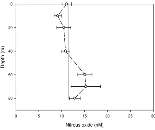
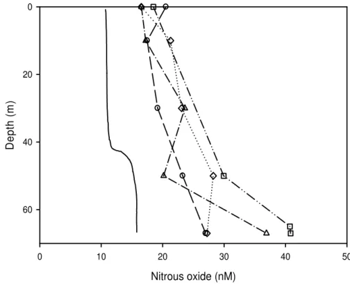
Concentration ranges and profiles were similar to open water concentrations found in other studies on lakes and reservoirs (Huttunen et al., 2003; Mengis
10
et al., 1996). Minimum concentration was 6 nM (55% saturation) in Lake Zeuzier and 41 nM (260% saturation) at the bottom of Lake Lungern. Fig-ure 2a and b show a typical profile for an alpine reservoir (Lake Grimsel) and for a lowland reservoir (Lake Lungern). The remaining profiles are documented in the electronic supplement (http://www.biogeosciences-discuss.net/5/3699/2008/
15
bgd-5-3699-2008-supplement.pdf, Figs. B1–B3).
Concentrations in the three alpine reservoirs were close to the atmospheric equilib-rium concentration in the water column. Although they differed from equilibrium con-centrations at the surface we assumed these alpine reservoirs to be neither a source nor a sink. Both lowland reservoirs were supersaturated with N2O throughout the
wa-20
ter column, being small nitrous oxide sources of 72±22µg m−2d−1(Lake Wohlen) and
50±13µg m−2d−1(Lake Lungern, all sampling campaigns).
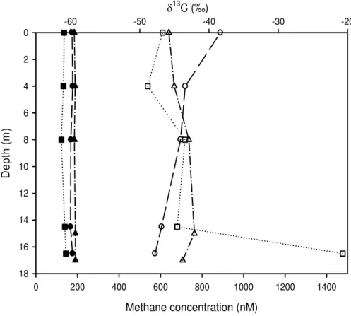
4.3 Methane concentrations,δ13C isotopic composition and emissions
In the following, we will group the reservoirs into three categories and illustrate the different categories with one example profile. The profiles of the remaining reservoirs
25
BGD
5, 3699–3736, 2008GHG emissions from alpine reservoirs
T. Diem et al.
Title Page
Abstract Introduction
Conclusions References
Tables Figures
◭ ◮
◭ ◮
Back Close
Full Screen / Esc
Printer-friendly Version
Interactive Discussion
5/3699/2008/bgd-5-3699-2008-supplement.pdf, Figs. A1–A7). The categories are:
(i) uniform methane profile (Lakes Oberaar, Dix, Bianco, Grimsel and Wohlen),
(ii) increasing methane concentrations towards the sediment (Lakes Sihl, Zeuzier, and Santa Maria),
5
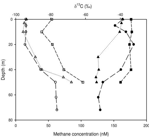
(iii) profiles with methane maxima in the water column (Lakes Luzzone, Lungern, and Gruy `ere).
(i) uniform methane profiles
10
To greater or lesser extent constant methane concentrations in the water column were found in these five reservoirs. In Lake Dix, concentrations were around 20 nM at most depths, and up to three times higher at certain depths (Fig. 3a). These depths coincided with small temperature perturbations and were most likely the result of inflowing water, stratifying in these layers (Fig. 3b). The water was warmer than
15
the remaining lake water because it was pumped from lower altitude reservoirs or neighbouring valleys into Lake Dix. While the δ13C values for most of the reservoir were between −40‰ and −37‰, at the depths with enhanced concentrations, the
δ13C also differed from the remainder of the reservoir, which supported the hypothesis of an external CH4 source. Sediments did not seem to contribute to the methane
20
content of the reservoir.
Concentrations in Lake Bianco were at saturation level (∼3 nM), hence the
methane emissions were negligible (see Table 2). The three other alpine reser-voirs Lake Dixence, Oberaar and Grimsel emitted methane at 0.05 mg m−2d−1, 0.28±0.03 mg m−2d−1, and 0.37±0.16 mg m−2d−1, respectively.
25
BGD
5, 3699–3736, 2008GHG emissions from alpine reservoirs
T. Diem et al.
Title Page
Abstract Introduction
Conclusions References
Tables Figures
◭ ◮
◭ ◮
Back Close
Full Screen / Esc
Printer-friendly Version
Interactive Discussion
Methane concentrations nearly doubled from the entrance of the reservoir to-wards the dam, where concentrations at the surface were 880 nM in May 2005 and around 650 nM for all other dates we sampled (Fig. 4). The profiles in the basin in front of the dam barrage were not uniform, in July 2005 and September 2006
5
concentrations increased towards the bottom and reached values of 1470 nM and 1000 nM respectively. Changes in concentrations within the year 2005 were marginal except for the barrage basin, where concentrations were about 300 nM higher.
The carbon isotopic composition changed little over the measurement period, but changes occurred with distance from the dam. Values at the entrance of the reservoir
10
were around−50‰, decreasing to−60‰ in the middle of the reservoir and at the dam.
Diffusive fluxes in Lake Wohlen were one order of magnitude higher than in the other reservoirs at 6.3±3.6 mg m−2d−1. As we noticed intense bubble flux in some
areas of the lake we also measured the ebullition flux from this reservoir with funnels. From these funnel measurements we found ebullition to account for an additional
15
900±700 mg CH4m− 2
d−1 (Range 200–2000 mg m−2d−1, Median 700 mg m−2d−1) (Electronic supplement Table C1). Assuming the area of intense bubble flux to be approximately one third of the reservoir, preliminary ebullition fluxes for Lake Wohlen would be 300±230 mg CH4m−
2
d−1. This is in the range of results Keller et al. (1994) and Galy-Lacaux et al. (1997) found for two tropical reservoirs, but more
20
than three times higher, than what dos Santos et al. (2006) found for reservoirs in Brazil or Duchemin et al. (1995) and Huttunen et al. (2002) for several boreal reservoirs.
(ii) increasing methane concentrations from the surface to the sediment
25
The reservoirs in this category had a more or less steady increase of methane concentrations from the water surface to the sediment surface in common. Con-centrations increased with a gradient close to 1 nmol m−1 (range 0.4–1.4) in Lakes Zeuzier and Santa Maria, and about ten times faster in the shallow Lake Sihl (range 5.4–12.8 nmol m−1). Methane diffusing from the sediment seems to be the cause for
BGD
5, 3699–3736, 2008GHG emissions from alpine reservoirs
T. Diem et al.
Title Page
Abstract Introduction
Conclusions References
Tables Figures
◭ ◮
◭ ◮
Back Close
Full Screen / Esc
Printer-friendly Version
Interactive Discussion
the higher concentrations at the lake bed.
In Lake Santa Maria, methane concentrations on all three sampling dates (June, July, and August) increased towards the bottom (Fig. 5a). In June surface concen-trations were 55 nM, while on the other two dates concenconcen-trations were about 15 nM. Concentrations right above the sediment decreased from June to August, from 100 nM
5
to 63 nM. Meanwhile the carbon isotopic signal of methane in June was−34‰ from the
surface down to 40 m and the decreased to−40‰. On the other two dates the value
at the surface was−40‰ and values decreased to−54‰ in July and−51‰ in August.
The rapid change in the isotopic composition is reflected in temperature (Fig. 5b) and other hydrographic parameters (data not shown) as well.
10
The emission flux was lowest in Lake Zeuzier at 0.07 mg m−2d−1, three times higher in Lake Sihl at 0.21±0.08 mg m−2d−1 and still higher in Lake Santa Maria at
0.32±0.29 mg m−2d−1. Emissions in Lake Santa Maria were highest in June 2005
with 0.65 mg m−2d−1, while in July and August values were similar to the ones in Lake Luzzone for the same time span (0.15±0.06 mg m−2d−1).
15
(iii) enhanced methane concentrations in an intermediate layer
Profile shapes in these reservoirs did not increase steadily from the water sur-face to the sediment, but a (local) maximum in methane concentrations was detected
20
in intermediate water layers. From the lower methane minimum downwards, concen-trations increased again towards the sediment. We suggest methane entering the reservoir with inflowing water stratifying at intermediary depth to be the reason for this profile shape.
Lake Luzzone was sampled twice in July and August 2005 (Fig. 6). Both times,
25
BGD
5, 3699–3736, 2008GHG emissions from alpine reservoirs
T. Diem et al.
Title Page
Abstract Introduction
Conclusions References
Tables Figures
◭ ◮
◭ ◮
Back Close
Full Screen / Esc
Printer-friendly Version
Interactive Discussion
−38 and−40‰ at the minima and−50 to−52‰ at higher concentrations.
Methane emissions from each lake individually were 0.15±0.02 mg m−2d−1,
0.13±0.12 mg m−2d−1and 0.13±0.01 mg m−2d−1for Lake Gruy `ere, Lake Lungern and
Lake Luzzone, respectively. Changes during the sampling period were small in Lake Gruy `ere and Lake Luzzone, while in Lake Lungern emissions decreased in the year
5
2006 from 0.34±0.08 mg m−2d−1in early August to 0.07±0.06 mg m−2d−1for four
sam-pling dates in September and October. The situation in Lake Lungern was special however, as due to a defect in that year large amounts of water supersaturated with air flowed into the lake. This resulted in air saturations of more than 150% and caused a mixing of the water body down to 40 m, while in normal years the epilimnion is only
10
10 m deep in summer (Jaun et al., 2006). However, emissions in October 2006 were not much lower than in October 2005, when no malfunction occurred.
4.4 Inflows and outflows
Methane concentrations of inflows and outflows are given in Table 2. Concentrations were supersaturated with methane for all sampling dates, with a range of 10 to 420 nM.
15
Methane loss at the turbine was calculated by using the concentration of the closest sampling point to the depth of the outlet. Concentrations did not differ before and after the turbine in Lakes Wohlen and Gruy `ere, while at Lakes Sihl, Luzzone and Grim-sel concentrations are between 16 and 73% lower after the water passed the turbine (Table 2).
BGD
5, 3699–3736, 2008GHG emissions from alpine reservoirs
T. Diem et al.
Title Page
Abstract Introduction
Conclusions References
Tables Figures
◭ ◮
◭ ◮
Back Close
Full Screen / Esc
Printer-friendly Version
Interactive Discussion
5 Discussion
5.1 Diffusive surface emissions
5.1.1 Carbon dioxide
Similar to other boreal and temperate reservoirs, CO2is the most important (in regard to volume and GWP) greenhouse gas emitted from Swiss reservoirs. The emissions
5
are in the same range as emissions from other temperate and boreal reservoirs (Ta-ble 3).
In their analysis Tremblay et al. (2005) found among others correlations between CO2 flux and the parameters pH and month of sampling. In our data (except for Lake Luz-zone), there is as well a correlation between CO2 flux and pH (R
2
=0.741,p<0.0001),
10
which can easily be explained by our calculation of the CO2 concentration from al-kalinity and pH. Another correlation existed between CO2 flux and date (R
2
=0.6137, p<0.0001). There is, however, no significant correlation between time and elevation for the three Lakes Wohlen, Gruy `ere and Sihl (ANOVA, F=6.6387, p=0.057). Both correlations are done with a low sample number (n=11) and have to be treated with
15
caution. The agreement with the findings of Tremblay et al. (2005), however, suggests the effect of season on CO2emissions to be real.
The date of separation was set somewhat arbitrarily, but for all lakes (except Lake Luzzone) emissions decreased from spring (May, early June) to summer, while pH increased during the same time (data not shown). This suggests a reduced CO2
emis-20
sion in summer, not from decreased DIC concentrations, but from a shift to bicarbonate and lower dissolved CO2concentrations.
5.1.2 Nitrous oxide
Similar to previous findings fluxes of N2O in lakes and reservoirs are small in open water (Huttunen et al., 2002) and are slightly higher in littoral zones (Huttunen et al.,
BGD
5, 3699–3736, 2008GHG emissions from alpine reservoirs
T. Diem et al.
Title Page
Abstract Introduction
Conclusions References
Tables Figures
◭ ◮
◭ ◮
Back Close
Full Screen / Esc
Printer-friendly Version
Interactive Discussion
2003). While emissions from the two lowland reservoirs are in the same range as previous results (Table 3), in the alpine reservoirs concentrations throughout the wa-ter column are very close to atmospheric equilibrium. Only N2O concentrations at the surface deviate from the equilibrium concentrations. There is no production of N2O in the deep alpine reservoirs we sampled and we assume calculated fluxes are
proba-5
bly overestimated. However, the amount of data from alpine reservoirs is limited and alpine reservoirs might be small sources and sinks for N2O as well, depending on the continuity of surface concentrations differing from the atmospheric equilibrium.
Overall, if we take the “Global Warming Potential” into account (for a 100 year time period the impact of N2O is about 12 times higher than the one of CH4; Forster et al.,
10
2007), the fluxes of N2O in the lowland lakes have the same warming potential as CH4.
5.1.3 Methane
All lakes except Lake Bianco were supersaturated with methane. Lake Bianco was saturated within measurement accuracy and does not emit methane to the atmosphere (Table 2).
15
If we separate the lakes into alpine, subalpine and lowland lakes and exclude Lake Wohlen, we get emissions of 0.25±0.17 mg m−2d−1, 0.21±0.21 mg m−2d−1 and
0.16±0.09 mg m−2d−1, respectively. There are no significant differences between the different elevation levels (ANOVA,F=1.651,p=0.21) and none between emissions and date.
20
In comparison to reservoirs from other regions (Table 3), emissions from the eleven Swiss reservoirs we sampled are more than one order of magnitude lower than emis-sions from temperate and boreal reservoirs and three orders of magnitude lower than methane emissions from tropical reservoirs. Only the diffusive flux from Lake Wohlen is in the same range as the ones from the temperate and boreal reservoirs, while the
25
BGD
5, 3699–3736, 2008GHG emissions from alpine reservoirs
T. Diem et al.
Title Page
Abstract Introduction
Conclusions References
Tables Figures
◭ ◮
◭ ◮
Back Close
Full Screen / Esc
Printer-friendly Version
Interactive Discussion
(i) the use of the thin boundary layer model (TBL) to calculate emissions
(ii) age of the reservoirs and
(iii) shape of the reservoirs
(i) Thin Boundary Layer method
5
It has been shown (Duchemin et al., 1999), that the TBL tends to underestimate fluxes as opposed to emissions measured by static chambers, especially in shallow water. In a comparison of the two methods, Matthews et al. (2003) found differences of more than an order of magnitude for very low wind speeds. They suggested
10
additional turbulences caused by the chambers to be the cause for this discrepancy. However, Soumis et al. (2004) found good agreement between the two methods for wind speeds under 3 m s−1, as did Gu ´erin et al. (2007) who let their chambers float free with the river to avoid additional turbulence. An underestimation in our fluxes can not be excluded; however, as both methods in most cases are within the same order
15
of magnitude the low fluxes we found seem reasonable.
The choice, which linear relationship is used to calculate the fluxes can also influence the results. We used the bi-linear relationship from Crusius and Wan-ninkhof (2003), and not the constant-linear one, since a comparison of these two showed only minor differences in emissions (data not shown). However, when we use
20
the relationship of Cole and Caraco (1998) differences between the lowland and the subalpine/alpine reservoirs are significant (ANOVA, F=6.415, p=0.0061), leading to higher emissions from lowland reservoirs.
(ii) Age
25
BGD
5, 3699–3736, 2008GHG emissions from alpine reservoirs
T. Diem et al.
Title Page
Abstract Introduction
Conclusions References
Tables Figures
◭ ◮
◭ ◮
Back Close
Full Screen / Esc
Printer-friendly Version
Interactive Discussion
that was present in the area. Emissions decline after two to three years (Galy-Lacaux et al., 1999) and reach a steady state at a much lower level after 10 years (Abril et al., 2005).
All reservoirs we investigated were older than 35 years at the date of the sampling (Table 1), thus emissions should have levelled offand reached their “base level” more
5
than twenty years ago. For reservoirs, that flooded areas rich in organic material the “base level” is maintained by the degradation of carbon stored in the flooded soil. The rather low emissions of the Swiss reservoirs could be an indication of low productivity of the reservoirs and a used up carbon stock in the sediments.
10
(iii) Reservoir shape
Another important factor in emissions from lakes and reservoirs is the shape of the basin. Duchemin et al. (1995) found emissions from deep parts of LaGrande-2 reservoir to be less than half of the emissions from shallow areas. Additionally
15
littoral zones from lakes and reservoirs have been identified as important areas for greenhouse gas emissions (Huttunen et al., 2003; Wang et al., 2007). The subalpine and alpine reservoirs in Switzerland were created in narrow gorges with steep slopes, thus the ratio of shallow to deep areas is very small in most cases. As a result littoral zones are small and of minor importance and low flux areas determine the overall
20
emissions.
5.2 Other emission pathways
5.2.1 Loss at the turbines
Another important emission pathway for reservoirs is the loss caused by the turbu-lence caused during turbine passage. Of the five lakes we sampled for
investigat-25
BGD
5, 3699–3736, 2008GHG emissions from alpine reservoirs
T. Diem et al.
Title Page
Abstract Introduction
Conclusions References
Tables Figures
◭ ◮
◭ ◮
Back Close
Full Screen / Esc
Printer-friendly Version
Interactive Discussion
and Lake Grimsel) was 46±18% (Range 16–73%), matching the findings of Kemenes
et al. (2007). Whereas at Lake Wohlen and Lake Gruy `ere the water drops only a few meters down to the river, for the other three reservoirs, the height difference between the dam and the river is several hundreds of meters. While this drop seems to create enough turbulence for the water to degas on its way down the pipe, the short drop
5
through the air does not seem to be sufficient for a measurable loss of gas.
If we use the average loss at the turbine to calculate the importance of this emis-sion path for the total methane flux, we receive 51±13% for the subalpine and alpine
reservoirs, while for Lake Sihl gas loss at the turbine accounts for 14±7% of the total
emissions at the time of the measurement.
10
5.2.2 Ebullition
Ebullition in Lake Wohlen is nearly two orders of magnitude higher than the diffusive surface flux and is thus the most important emission pathway of methane in this reser-voir. We believe the high input of organic matter caused by the short water residence time of this run-of-the-river reservoir and subsequent anaerobic degradation is the
15
source of the high bubble flux and the high methane emissions compared to the other Swiss reservoirs. Given the low methane concentrations, especially in alpine reservoirs we do not expect ebullition in these reservoirs.
5.3 Methane sources
Generally, the carbon cycle in oxic lakes and reservoirs assumes methane production
20
in the sediments and methane oxidation, while methane is diffusing from the sediments into the water column (Kuivila et al., 1988). This oxidation can be traced with the increasingδ13C of methane (Barker and Fritz, 1981; Whiticar, 1999). Concentration and isotopic composition profiles in the lowland reservoirs agree well with this trend. Alpine reservoirs, on the other hand, did not show this behaviour and there seems to
25
BGD
5, 3699–3736, 2008GHG emissions from alpine reservoirs
T. Diem et al.
Title Page
Abstract Introduction
Conclusions References
Tables Figures
◭ ◮
◭ ◮
Back Close
Full Screen / Esc
Printer-friendly Version
Interactive Discussion
We, therefore, assume external sources to be responsible for the methane content in the alpine reservoirs. Most alpine reservoirs collect additional water from neighbour-ing valleys, which is transported there via tubes and in some cases pumped up from lower altitude. Methane concentration measurements in the retention basin Carassina of Lake Luzzone for example were 120 nM below the surface and 270 nM at the
bot-5
tom of the basin in August. Enhanced methane concentrations (Fig. 6) and enhanced conductivity (data not shown) are characteristic for the intermediate layer in Lake Luz-zone originating in a mixture of different inflows (among them water from the Basin Carrasina).
The only high alpine reservoir we have inflow data for is Lake Oberaar. Here,
10
methane concentrations of the water flowing from the glacier into the reservoir reach 30 nM in August with values in June and July are lower (around 15 nM), possibly due to dilution by snow melt water. Concentrations and isotopic composition of the inflowing water (Table 2) are very similar to the values in the lake (Electronic supplement Fig. A7). It has been shown, that methane can be produced in glaciers and low temperature
en-15
vironments (e.g. Price, 2007; Wadham et al., 2008) Theδ13C value of−35‰ suggests
that, methane produced in the glacier has already been partially oxidized by the time it left the glacier snout.
Not only in alpine reservoirs are inflows important for the methane content in and the emissions from the reservoirs. Estimating methane inflow from the river Jogne
20
and Sarine into Lake Gruy `ere and comparing it to methane emissions shows that 4.8 and 1.5 times more methane enters the reservoir in May and June, respectively than leaves the reservoir via surface diffusion. Only in August was diffusion five times higher than methane inflow. It seems that during late spring and early summer methane diffusing from the lake surface originates mostly from reservoir inflows, while in autumn,
25
when the water mixes and in spring, before the reservoir is stratified methane from the sediment is more important.
BGD
5, 3699–3736, 2008GHG emissions from alpine reservoirs
T. Diem et al.
Title Page
Abstract Introduction
Conclusions References
Tables Figures
◭ ◮
◭ ◮
Back Close
Full Screen / Esc
Printer-friendly Version
Interactive Discussion
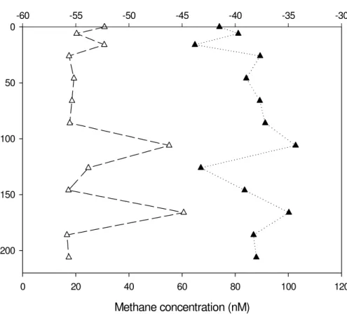
methane is already oxidized before it reaches the water column. This is reflected in the isotopic composition with values from−55‰ to−20‰. Methane flux from the
sed-iments in the middle basin of Lake Lungern, calculated from the methane concentra-tion profile (Electronic supplement Fig. A2b), was 410µmol m−2d−1, similar to the flux found in aerobic Lake Constance (Frenzel et al., 1990). Methane oxidation consumed
5
93% of the methane diffusing upwards in the sediment at Lake Constance and a sim-ilar rate is to be expected in the reservoirs we sampled, as at Lake Lungern methane concentrations in the water above the sediment were always lower than 80 nM.
5.4 Origin of methane in the inflows
To determine where the methane in the inflow originates from, we measured
concen-10
trations upstream and downstream of a wastewater treatment of the Sarine, an inflow of Lake Gruy `ere, and the river Minster, an inflow of Lake Sihl. While concentrations in the Sarine did not change or decreased slightly after the inlet of the cleaned wastewater, concentrations in the Minster increased 2–5 times together with a decrease ofδ13C of up to 20‰, indicating biologically produced methane in the outflow of the wastewater
15
treatment plant.
One of the major inflows of Lake Sihl, the river Minster, crosses a plain of agricultur-ally used land. At the sampling date in August we measured methane concentrations at the beginning of the plain and after the plain at the inflow to the lake. Methane concentration rose more than 10-fold to 367 nM after the passage of the plain and the
20
carbon isotope signal fell from−39‰ to−56‰. Thus the main source of methane in
the river Minster lies within this agricultural influenced plain.
6 Conclusions
The most important greenhouse gas emitted from perialpine and alpine reservoirs in Switzerland is CO2. On average, reservoir emissions are 860±700 mg m−
2
d−1 and
BGD
5, 3699–3736, 2008GHG emissions from alpine reservoirs
T. Diem et al.
Title Page
Abstract Introduction
Conclusions References
Tables Figures
◭ ◮
◭ ◮
Back Close
Full Screen / Esc
Printer-friendly Version
Interactive Discussion
therefore slightly smaller than emissions from boreal and temperate reservoirs in other parts of the world. Emissions in the spring time were higher than in summer and autumn (p<0.0001), while no elevation effect could be found.
Alpine reservoirs were in equilibrium with atmospheric N2O concentrations, whereas two lowland reservoirs emitted small amounts of N2O at 72±22µg m−2d−1.
5
Methane emissions were an order of magnitude smaller than values pub-lished for reservoirs in temperate and boreal climates. Average emissions were 0.2±0.15 mg m−2d−1 for all reservoirs, except Lake Wohlen, which emitted
1.5±0.4 mg m−2d−1 via surface diffusion and 300±230 mg m−2d−1 via bubble flux.
There was no significant difference between different elevations, as higher wind speeds
10
at higher elevations compensated the lower methane concentrations. The amount of external methane entering via inflows is sufficient to explain the emission rates found in most reservoirs. Methane input from sediments is only of minor importance for open water sites. Only during times of mixing can accumulated methane in the water layers above the sediment contribute significantly to methane emission. The isotopic
compo-15
sition of sedimentary methane suggests a biogenic source and partial oxidation. Methane loss at the turbine accounted for around 50% of total emissions (diffusive surface flux+gas loss at the turbine) in subalpine and alpine reservoirs. This type of emissions was less important in lowland reservoirs such as Lake Sihl, where it con-tributed only 14% of the total CH4flux to the atmosphere.
20
In two lowland reservoirs with a small height difference (smaller than 10m) between reservoir and receiving river, no additional emissions at the turbine were found.
Acknowledgements. We would like to thank MeteoSchweiz for supplying wind speed data. Funding by internal EAWAG funds is gratefully acknowledged. Additionally we would like to thank M. Fette, M. Schurter, M. Meyer, I. Ostrovsky, D. Finger and L. Jaun for their assistance
25
BGD
5, 3699–3736, 2008GHG emissions from alpine reservoirs
T. Diem et al.
Title Page
Abstract Introduction
Conclusions References
Tables Figures
◭ ◮
◭ ◮
Back Close
Full Screen / Esc
Printer-friendly Version
Interactive Discussion
References
Abril, G., Gu ´erin, F., Richard, S., Delmas, R., Galy-Lacaux, C., Gosse, P., Tremblay, A., Var-falvy, L., Santos, M. A. D., and Matvienko, B.: Carbon dioxide and methane emissions and the carbon budget of a 10-year old tropical reservoir (Petit Saut, French Guiana), Global Biogeochem. Cy., 19, GB4007, doi:10.1029/2005GB002457, 2005.
5
Abril, G., Richard, S., and Gu ´erin, F.: In situ measurements of dissolved gases (CO2 and CH4) in a wide range of concentrations in a tropical reservoir using an equilibrator, Sci. Total Environ., 354, 246–251, 2006.
Barker, J. F. and Fritz, P.: Carbon isotope fractionation during microbial methane oxidation, Nature, 293, 289–291, 1981.
10
Cole, J. J. and Caraco, N. F.: Atmospheric exchange of carbon dioxide in a low-wind oligotrophic lake measured by the addition of SF6, Limnol. Oceanogr., 43, 647–656, 1998.
Crusius, J. and Wanninkhof, R.: Gas transfer velocities measured at low wind speed over a lake, Limnol. Oceanogr., 48, 1010–1017, 2003.
de Angelis, M. A. and Lilley, M. D.: Methane in surface waters of Oregon estuaries and rivers,
15
Limnol. Oceanogr., 32, 716–722, 1987.
dos Santos, M. A., Rosa, L. P., Sikar, B., Sikar, E., and dos Santos, E. O.: Gross greenhouse gas fluxes from hydro-power reservoir compared to thermo-power plants, Energ. Policy, 34, 481–488, 2006.
Duchemin, E., Lucotte, M., Canuel, R., and Chamberland, A.: Production of the greenhouse
20
gases CH4 and CO2 by hydroelectric reservoirs of the boreal region, Global Biogeochem. Cy., 9, 529–540, 1995.
Duchemin, E., Lucotte, M., and Canuel, R.: Comparison of static chamber and thin boundary layer equation methods for measuring greenhouse gas emissions from large water bodies, Environ. Sci. Technol., 33, 350–357, 1999.
25
Fearnside, P. M.: Greenhouse-gas emissions from Amazonian hydroelectric reservoirs: the example of Brazil’s Tucuru´ıDam as compared to fossil fuel alternatives, Environ. Conserv., 24, 64–75, 1997.
Fearnside, P. M.: Greenhouse gas emissions from a hydroelectric reservoir (Brazil’s Tucuru´ı
Dam) and the energy policy implications, Water Air Soil Pollut., 133, 69–96, 2002.
30
BGD
5, 3699–3736, 2008GHG emissions from alpine reservoirs
T. Diem et al.
Title Page
Abstract Introduction
Conclusions References
Tables Figures
◭ ◮
◭ ◮
Back Close
Full Screen / Esc
Printer-friendly Version
Interactive Discussion
Changes in Atmospheric Constituents and Radiative Forcing, in: Climate Change 2007: the physical science basis, Contribution of Working Group I to the Fourth Assessment Report of the Intergovernmental Panel on Climate Change, edited by: Solomon, S., Qin, D., Manning, M., Chen, Z., Marquis, M., Averyt, K. B., Tignor, M., and Miller, H. L., Cambridge University Press, Cambridge, UK and New York, NY, USA, 2007.
5
Frenzel, P., Thebrath, B., and Conrad, R.: Oxidation of methane in the oxic surface layer of a deep lake sediment (Lake Constance), FEMS Microbiol. Ecol., 73, 149–158, 1990.
Galy-Lacaux, C., Delmas, R., Jambert, C., Dumestre, J. F., Labroue, L., Richard, S., and Gosse, P.: Gaseous emissions and oxygen consumption in hydroelectric dams: A case study in French Guyana, Global Biogeochem. Cy., 11, 471–483, 1997.
10
Galy-Lacaux, C., Delmas, R., Kouadio, G., Richard, S., and Gosse, P.: Long-term greenhouse gas emissions from hydroelectric reservoirs in tropical forest regions, Global Biogeochem. Cy., 13, 503–517, 1999.
Gu ´erin, F., Abril, G., Serc¸a, D., Delon, C., Richard, S., Delmas, R., Tremblay, A., and Varfalvy, L.: Gas transfer velocities of CO2and CH4in a tropical reservoir and its river downstream, J.
15
Marine Syst., 66, 161–172, 2007.
Huttunen, J. T., V ¨ais ¨anen, T. S., Hellsten, S. K., Heikkinen, M., Nyk ¨anen, H., Jungner, H., Niskanen, A., Virtanen, M. O., Lindqvist, O. V., Nenonen, O. S., and Martikainen, P. J.: Fluxes of CH4, CO2, and N2O in hydroelectric reservoirs Lokka and Porttipahta in the northern boreal zone in Finland, Global Biogeochem. Cy., 16, 1003, doi:10.1029/2000GB001316,
20
2002.
Huttunen, J. T., Juutinen, S., Alm, J., Larmola, T., Hammar, T., Silvola, J., and Martikainen, P. J.: Nitrous oxide flux to the atmosphere from the littoral zone of a boreal lake, J. Geophys. Res.-Atmos., 108, 4421, doi:10.1029/2002JD002989, 2003.
Jaun, L., Ostrovsky, I., M ¨uller, B., Diem, T., Reinhardt, M., and W ¨uest, A.: Massive
25
Luft ¨ubers ¨attigung im Lungerersee vom Juni bis August 2006, EAWAG, Kastanienbaum, Switzerland, 2006.
Keller, M. and Stallard, R. F.: Methane emissions by bubbling from Lake Gattun, Panama, J. Geophys. Res., 99, 8307–8319, 1994.
Kelly, C. A., Rudd, J. W. M., St. Louis, V. L., and Moore, T.: Turning attention to reservoir
30
surfaces, a neglected area in greenhouse studies, EOS, 75, 332–333, 1994.
BGD
5, 3699–3736, 2008GHG emissions from alpine reservoirs
T. Diem et al.
Title Page
Abstract Introduction
Conclusions References
Tables Figures
◭ ◮
◭ ◮
Back Close
Full Screen / Esc
Printer-friendly Version
Interactive Discussion
Knox, M., Quay, P. D., and Wilbur, D.: Kinetic Isotopic Fractionation During Air-Water Gas Transfer of O2, N2, CH4, and H2, J. Geophys. Res.-Oceans, 97, 20 335–20 343, 1992. Kuivila, K. M., Murray, J. W., Devol, A. H., Lidstrom, M. E., and Reimers, C. E.: Methane Cycling
in the Sediments of Lake Washington, Limnol. Oceanogr., 33, 571–581, 1988.
Lima, I. B. T.: Biogeochemical distinction of methane releases from two Amazon
hydroreser-5
voirs, Chemosphere, 59, 1697–1702, 2005.
Liss, P. S. and Merlivat, L.: Air-sea gas exchange rates: Introduction and synthesis, in: The role of air-sea exchange in geochemical cycling, edited by: Buat-Menard, P. E., Reidel, Dordrecht, The Netherlands, 1986.
Matthews, C. J. D., St. Louis, V. L., and Hesslein, R. H.: Comparison of three techniques used
10
to measure diffusive gas exchange from sheltered aquatic surfaces, Environ. Sci. Technol., 37, 772–780, 2003.
McAuliffe, C.: GC determination of solutes by multiple phase equilibration, Chem. Technol., 46–51, 1971.
Mengis, M., G ¨achter, R., and Wehrli, B.: Nitrous oxide emissions to the atmosphere from an
15
artificially oxygenated lake, Limnol. Oceanogr., 41, 548–553, 1996.
Neal, C., House, W. A., and Down, K.: An assessment of excess carbon dioxide partial pressures in natural waters based in pH and alkalinity measurements, Sci. Total Environ., 210/211, 173–185, 1998.
Plummer, L. N. and Busenberg, E.: The Solubilities of Calcite, Aragonite and Vaterite in Co2
-20
H2O Solutions between 0 and 90◦C, and an Evaluation of the Aqueous Model for the System CaCO3-CO2-H2O, Geochim. Cosmochim. Ac., 46, 1011–1040, 1982.
Price, P. B.: Microbial life in glacial ice and implications for a cold origin of life, FEMS Microbiol. Ecol., 59, 217–231, 2007.
Rosa, L. P., Dos Santos, M. A., Matvienko, B., Sikar, E., Lourenc¸o, R. S. M., and Menezes,
25
C. F.: Biogenic gas production from major Amazon reservoirs, Brazil, Hydrol. Process., 17, 1443–1450, 2003.
Rosa, L. P., dos Santos, M. A., Matvienko, B., dos Santos, E. O., and Sikar, E.: Greenhouse gas emissions from hydroelectric reservoirs in tropical regions, Climatic Change, 66, 9–21, 2004.
30
Rudd, J. W. M., Harris, R., Kelly, C. A., and Hecky, R. E.: Are Hydroelectric Reservoirs Signifi-cant Sources of Greenhouse Gases?, Ambio, 22, 246–248, 1993.
BGD
5, 3699–3736, 2008GHG emissions from alpine reservoirs
T. Diem et al.
Title Page
Abstract Introduction
Conclusions References
Tables Figures
◭ ◮
◭ ◮
Back Close
Full Screen / Esc
Printer-friendly Version
Interactive Discussion
methane in water and gas, Anal. Chem., 69, 40–44, 1997.
Smith, L. K., and Lewis Jr., W. M.: Seasonality of methane emissions from five lakes and associated wetlands of the Colorado Rockies, Global Biogeochem. Cy., 6, 323–338, 1992. St. Louis, V. L., Kelly, C. A., Duchemin, E., Rudd, J. W. M., and Rosenberg, D. M.: Reservoir
surfaces as sources of greenhouse gases to the atmosphere: a global estimate, Bioscience,
5
50, 766–775, 2000.
Tremblay, A., Therrien, J., Hamlin, B., Wichmann, E., and LeDrew, L. J.: GHG Emissions from Boreal Reservoirs and Natural Aquatic Ecosystems, in: Greenhouse Gas Emissions – Fluxes and Processes, edited by: Tremblay, A., Varfalvy, L., Roehm, C., and Garneau, M., Environmental Science, Springer, Berlin, Germany, 2005.
10
Wadham, J. L., Tranter, M., Tulaczyk, S., and Sharp, M.: Subglacial methanogenesis: A poten-tial climatic amplifier?, Global Biogeochem. Cy., 22, GB2021, doi:10.1029/2007GB002951, 2008.
Wang, H., Yang, L., Wang, W., Lu, J., and Yin, C.: Nitrous oxide (N2O) flixes and their re-lationships with water-sediment characteristics in a hyper-eutrophic shallow lake, China, J.
15
Geophys. Res., 112, G01005, doi:10.1029/2005JG000129, 2007.
Wanninkhof, R.: Relationship between wind speed and gas exchange over the ocean, J. Geo-phys. Res., 97, 7373–7382, 1992.
Weiss, R. F.: Carbon dioxide in water and sewater: the solubility of a non-ideal gas, Mar. Chem., 2, 203–215, 1974.
20
Weiss, R. F. and Price, B. A.: Nitrous oxide solubility in water and seawater, Mar. Chem., 8, 347–359, 1980.
Whiticar, M. J., Faber, E., and Schoell, M.: Biogenic methane formation in marine and fresh-water environments: CO2 resduction vs. acetate fermentation-Isotope evidence, Geochim. Cosmochim. Ac., 50, 693–709, 1986.
25
Whiticar, M. J.: Carbon and hydrogen isotope systematics of bacterial formation and oxidation of methane, Chem. Geol., 161, 291–314, 1999.
BGD
5, 3699–3736, 2008GHG emissions from alpine reservoirs
T. Diem et al.
Title Page
Abstract Introduction
Conclusions References
Tables Figures
◭ ◮
◭ ◮
Back Close
Full Screen / Esc
Printer-friendly Version
Interactive Discussion
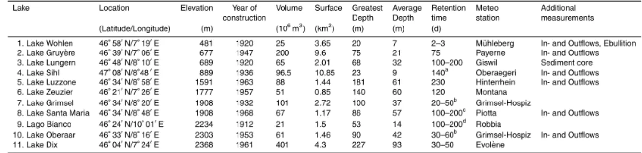
Table 1.Properties of the sampled reservoirs.
Lake Location Elevation Year of Volume Surface Greatest Average Retention Meteo Additional
construction Depth Depth time station measurements
(Latitude/Longitude) (m) (106m3) (km2) (m) (m) (d)
1. Lake Wohlen 46◦
58′
N/7◦
19′
E 481 1920 25 3.65 20 7 2–3 M ¨uhleberg In- and Outflows, Ebullition
2. Lake Gruy `ere 46◦39′N/7◦06′E 677 1947 200 9.6 75 21 75 Payerne In- and Outflows
3. Lake Lungern 46◦48′N/8◦10′E 689 1920 65 2.01 68 32 100–200 Giswil Sediment core
4. Lake Sihl 47◦08′N/8◦48′E 889 1936 96.5 10.85 23 9 140a Oberaegeri In- and Outflows
5. Lake Luzzone 46◦34′N/8◦58′E 1591 1963 88 1.44 181 61 230 Hinterrhein In- and Outflows
6. Lake Zeuzier 46◦21′N/7◦26′E 1777 1957 51 0.85 140 60 120 Montana
7. Lake Grimsel 46◦34′N/8◦20′E 1908 1932 101 2.72 100 37 20–50b Grimsel-Hospiz
8. Lake Santa Maria 46◦
34′
N/8◦
48′
E 1908 1968 67 1.17 86 57 100–200c Piotta In- and Outflows
9. Lago Bianco 46◦24′N/10◦01′E 2234 1912 21 1.5 53 14 100–200d Robbia
10. Lake Oberaar 46◦33′N/8◦16′E 2303 1953 61 1.46 90 42 30–60b Grimsel-Hospiz In- and Outflows
11. Lake Dix 46◦04′N/7◦24′E 2368 1961 401 4.3 227 93 30–50 Evol `ene
aabout 10% of the water in the Lake are pumped from Lake Zurich
bwater from Lake Grimsel is pumped into Lake Oberaar at night and released back to Lake Grimsel during the day for energy production;
this way the volume of Lake Oberaar gets replaced about ten times every year
cis connected with two other reservoirs to one power station
d
BGD
5, 3699–3736, 2008GHG emissions from alpine reservoirs
T. Diem et al.
Title Page
Abstract Introduction
Conclusions References
Tables Figures
◭ ◮
◭ ◮
Back Close
Full Screen / Esc
Printer-friendly Version
Interactive Discussion
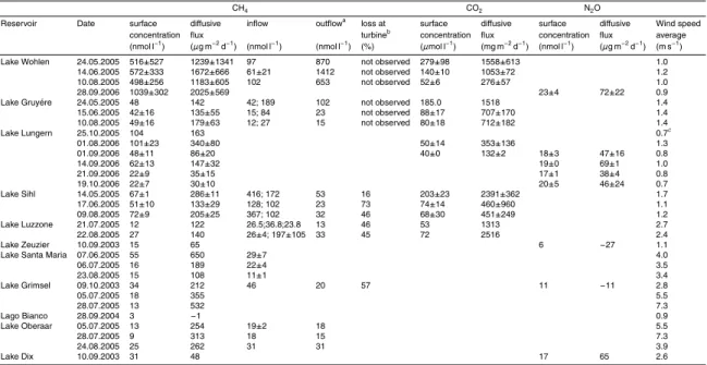
Table 2.Diffusive fluxes of CH4, CO2and N2O in the studied reservoirs and average wind speed on the sampling dates.
CH4 CO2 N2O
Reservoir Date surface diffusive inflow outflowa loss at surface di
ffusive surface diffusive Wind speed concentration flux turbineb concentration flux concentration flux average
(nmol l−1) (
µg m−2d−1) (nmol l−1) (nmol l−1) (%) (
µmol l−1) (mg m−2d−1) (nmol l−1) (
µg m−2d−1) (m s−1)
Lake Wohlen 24.05.2005 516±527 1239±1341 97 870 not observed 279±98 1558±613 1.0 14.06.2005 572±333 1672±666 61±21 1412 not observed 140±10 1053±72 1.2 10.08.2005 498±256 1183±605 102 653 not observed 52±6 276±57 1.0
28.09.2006 1039±302 2025±569 23±4 72±22 0.9
Lake Gruy ´ere 24.05.2005 48 142 42; 189 102 not observed 185.0 1518 1.4 15.06.2005 42±16 135±55 15; 84 23 not observed 88±17 707±170 1.4 10.08.2005 49±16 179±63 12; 27 15 not observed 80±18 712±182 1.4
Lake Lungern 25.10.2005 104 163 0.7c
01.08.2006 101±23 340±80 50±14 353±136 1.3
01.09.2006 48±11 86±20 40±0 132±2 18±3 47±16 0.8
14.09.2006 62±13 147±32 19±0 69±1 1.0
21.09.2006 22±9 35±15 17±1 38±4 0.8
19.10.2006 22±7 30±10 20±5 46±24 0.7
Lake Sihl 14.05.2005 67±1 286±11 416; 172 53 16 203±23 2391±362 1.7 17.06.2005 51±10 133±29 128; 102 23 73 74±14 460±960 1.1 09.08.2005 72±9 205±25 367; 102 32 46 68±30 451±249 1.2
Lake Luzzone 21.07.2005 12 122 26.5;36.8;23.8 13 46 53 1313 2.7
22.08.2005 27 140 26±4; 197±105 33 45 72 2516 2.4
Lake Zeuzier 10.09.2003 15 65 6 −27 1.1
Lake Santa Maria 07.06.2005 55 650 29±7 4.0
06.07.2005 16 189 22±4 3.5
23.08.2005 15 108 11±1 3.4
Lake Grimsel 09.10.2003 34 212 46 20 57 11 −11 2.8
05.07.2005 18 355 5.5
28.07.2005 13 532 7.3
Lago Bianco 28.09.2004 3 −1 0.9
Lake Oberaar 05.07.2005 13 254 19±2 18 5.5
28.07.2005 9 313 18 15 7.3
24.08.2005 25 262 31 31 3.9
Lake Dix 10.09.2003 31 48 17 65 2.6
a
measured after the water passed the turbine
bcalculated from the di
fference of the methane concentrations closest to the depth of the outlet and the outflow concentration
BGD
5, 3699–3736, 2008GHG emissions from alpine reservoirs
T. Diem et al.
Title Page
Abstract Introduction
Conclusions References
Tables Figures
◭ ◮
◭ ◮
Back Close
Full Screen / Esc
Printer-friendly Version
Interactive Discussion
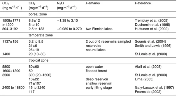
Table 3.Greenhouse gas emissions from reservoirs in different climates.
CO2 CH4 N2O Remarks Reference
(mg m−2 d−1
) (mg m−2 d−1
) (mg m−2 d−1
)
boreal zone
1508±1771 8.8±12 −1.38 to 3.10 Tremblay et al. (2005)
≈1200 5 to 10 Duchemin et al. (1995)
504–3192 2.5 to 133 −0.089 to 0.270 two Finnish lakes Huttunen et al. (2002)
temperate zone
1137±156 3.2 to 9.5 2 out of 6 reservoirs sampled Soumis et al. (2004)
21±6 reservoirs Smith and Lewis (1996)
26±19 natural lakes
1400 20 (10–80) St.Louis et al. (2000)
tropical zone
5800 80±60 open water Abril et al. (2005)
1600±1300 50 flooded forest
3500 300 (20–1500) St.Louis et al. (2000)
13±22 deep reservoir Lima (2005)
71±107 shallow reservoir
2400 to 18800 15 to 3240 early filling stage Galy-Lacaux et al. (1997)
BGD
5, 3699–3736, 2008GHG emissions from alpine reservoirs
T. Diem et al.
Title Page
Abstract Introduction
Conclusions References
Tables Figures
◭ ◮
◭ ◮
Back Close
Full Screen / Esc
Printer-friendly Version
Interactive Discussion
BGD
5, 3699–3736, 2008GHG emissions from alpine reservoirs
T. Diem et al.
Title Page
Abstract Introduction
Conclusions References
Tables Figures
◭ ◮
◭ ◮
Back Close
Full Screen / Esc
Printer-friendly Version
Interactive Discussion Nitrous oxide (nM)
0 5 10 15 20 25 30
D
ept
h (
m
)
0
20
40
60
80
BGD
5, 3699–3736, 2008GHG emissions from alpine reservoirs
T. Diem et al.
Title Page
Abstract Introduction
Conclusions References
Tables Figures
◭ ◮
◭ ◮
Back Close
Full Screen / Esc
Printer-friendly Version
Interactive Discussion Nitrous oxide (nM)
0 10 20 30 40 50
D
ept
h (
m
)
0
20
40
60
BGD
5, 3699–3736, 2008GHG emissions from alpine reservoirs
T. Diem et al.
Title Page
Abstract Introduction
Conclusions References
Tables Figures
◭ ◮
◭ ◮
Back Close
Full Screen / Esc
Printer-friendly Version
Interactive Discussion Methane concentration (nM)
0 20 40 60 80 100 120
0
50
100
150
200
δ13
C (‰)
-60 -55 -50 -45 -40 -35 -30
BGD
5, 3699–3736, 2008GHG emissions from alpine reservoirs
T. Diem et al.
Title Page
Abstract Introduction
Conclusions References
Tables Figures
◭ ◮
◭ ◮
Back Close
Full Screen / Esc
Printer-friendly Version
Interactive Discussion
Temperature (°C)
4.8 4.9 5.0 5.1 5.2 5.3
D
ept
h (
m
)
0
50
100
150
200
BGD
5, 3699–3736, 2008GHG emissions from alpine reservoirs
T. Diem et al.
Title Page
Abstract Introduction
Conclusions References
Tables Figures
◭ ◮
◭ ◮
Back Close
Full Screen / Esc
Printer-friendly Version
Interactive Discussion
Methane concentration (nM)
0 200 400 600 800 1000 1200 1400
Dep
th
(
m
)
0
2
4
6
8
10
12
14
16
18
-60 -50 -40 -30 -20
δ13
C (‰)
BGD
5, 3699–3736, 2008GHG emissions from alpine reservoirs
T. Diem et al.
Title Page
Abstract Introduction
Conclusions References
Tables Figures
◭ ◮
◭ ◮
Back Close
Full Screen / Esc
Printer-friendly Version
Interactive Discussion
Methane concentration (nM)
0 50 100 150 200
De
pt
h
(
m
)
0
20
40
60
80
-100 -80 -60 -40
δ13
C (‰)
BGD
5, 3699–3736, 2008GHG emissions from alpine reservoirs
T. Diem et al.
Title Page
Abstract Introduction
Conclusions References
Tables Figures
◭ ◮
◭ ◮
Back Close
Full Screen / Esc
Printer-friendly Version
Interactive Discussion Temperature (°C)
4 5 6 7 8 9 10 11 12
D
e
pt
h (
m
)
0
20
40
60
80
BGD
5, 3699–3736, 2008GHG emissions from alpine reservoirs
T. Diem et al.
Title Page
Abstract Introduction
Conclusions References
Tables Figures
◭ ◮
◭ ◮
Back Close
Full Screen / Esc
Printer-friendly Version
Interactive Discussion
Methane concentration (nM)
0 20 40 60 80 100 120
D
ept
h (
m
)
0
20
40
60
80
100
120
δ13
C (‰)
-100 -80 -60 -40