Development of a iron pipe corrosion simulation model for a water supply network

(1)

DWESD

5, 85–120, 2012

Development of a iron pipe corrosion

simulation model

M. Bernats et al.

Title Page

Abstract Introduction

Conclusions References

Tables Figures

◭ ◮

Back Close

Full Screen / Esc

Printer-friendly Version Interactive Discussion

Discussion

P

a

per

|

Dis

cussion

P

a

per

|

Discussion

P

a

per

|

Discussio

n

P

a

per

|

Drink. Water Eng. Sci. Discuss., 5, 85–120, 2012 www.drink-water-eng-sci-discuss.net/5/85/2012/ doi:10.5194/dwesd-5-85-2012

Drinking Water

Engineering and Science

Discussions

O

p

en

Acc

e

s

This discussion paper is/has been under review for the journal Drinking Water Engineering and Science (DWES). Please refer to the corresponding final paper in DWES if available.

Development of a iron pipe corrosion

simulation model for a water supply

network

M. Bernats1, S. W. Osterhus2, K. Dzelzitis3, and T. Juhna1

1

Department of Water Engineering and Technology, Riga Technical University, Latvia

2

Department of Hydraulic and Environmental Engineering, Norwegian University of Science and Technology, Norway

3

Department of Composite Materials and Structures, Riga Technical University, Latvia

Received: 17 February 2012 – Accepted: 19 March 2012 – Published: 2 April 2012

Correspondence to: T. Juhna (talis.juhna@rtu.lv)

(2)

DWESD

5, 85–120, 2012

M. Bernats et al.

Title Page

Tables Figures

◭ ◮

Back Close

Full Screen / Esc

Discussion

P

a

per

|

Dis

cussion

P

a

per

|

Discussion

P

a

per

|

Discussio

n

P

a

per

|

Abstract

Corrosion in water supply networks is unwanted process that causes pipe material loss and subsequent pipe failures. Nowadays pipe replacing strategy most often is based on pipe age, which is not always the most important factor in pipe burst rate. In this study a methodology for developing a mathematical model to predict the decrease

5

of pipe thickness in a large cast iron networks is presented. The quality of water, the temperature and the water flow regime were the main factors taken into account in the corrosion model. The water quality and flow rate effect were determined by measuring corrosion rate of metals coupons over the period of one year at different flow regimes. The obtained constants were then introduced in a calibrated hydraulic

10

model (Epanet) and the corrosion model was validated by measuring the decrease of wall thickness in the samples that were removed during the regular pipe replacing event. The validated model was run for 30 yr to simulate the water distribution system of Riga (Latvia). Corrosion rate in the first year was 8.0–9.5 times greater than in all the forthcoming years, an average decrease of pipe wall depth being 0.013/0.016 mm per

15

year in long term. The optimal iron pipe exploitation period was concluded to be 30– 35 yr (for pipe wall depth 5.50 mm and metal density 7.5 m3t−1). The initial corrosion model and measurement error was 33 %. After the validation of the model the error was reduced to below 15 %.

1 Introduction

20

Iron pipe corrosion in water distribution networks is of a special concern for the drinking water industry, because of the large amount of unlined iron pipes that are in use nowa-days. Corrosion consumes oxidants and disinfectants used for water treatment, create scales and loose deposits that increase the energy required for pumping, facilitates biofilm growth, and causes the discoloration of water (AWWA, 1996; Juhna, 2009).

25

(3)

DWESD

5, 85–120, 2012

M. Bernats et al.

Title Page

Tables Figures

◭ ◮

Back Close

Full Screen / Esc

Discussion

P

a

per

|

Dis

cussion

P

a

per

|

Discussion

P

a

per

|

Discussio

n

P

a

per

|

loss of revenue for water industry (AWWA, 2010). Presently pipe replacing strategy is most often based on the age of pipes, which is not always the most important factor in pipe burst rate. There are several attempts described in literature (Sarin et al., 2001; Naser et al., 2007; Vargas et al., 2010) to predict the corrosion rate of pipes and to bet-ter plan the anticorrosion and pipe replacing strategy. However due to the complexity

5

of the corrosion phenomena and many unknown factors the application of mechanistic models has not been successful. On the other hand the use of empirical model is also problematic as it takes into account only the situation representing the period of the measurements however the extrapolation of the results is not always possible.

The objectives of this study were to create a corrosion model, based on the physical

10

and chemical properties of water flow and to validate the model in a large scale water supply network.

In this paper the methodology for developing and validating of model to predict pipe material loss using limited number of sampling points is presented. The accuracy can be continuously improved by adding more sampling points. The study was carried in

15

Riga, Latvia over the period of one year. The major limitation of the model is that it is not able to distinguish between pit and homogenous corrosion.

2 Materials and methods

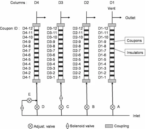
2.1 Tests with corrosion rigs

To measure corrosion rates test rig experiments were carried out for the water

treat-20

ment plants (WTP) of Riga city. One experiment was done at the WTP supplied by surface water (D), other at WTP supplied by groundwater (B). Test rigs were placed in water flow directly after WTPs. Corrosion rates were determined from measurements of weight loss of coupons (low grade steel st37) for duration of 12 months. Figure 1 shows schematic drawing of corrosion rate experiment with test rigs. Setup, shown

25

(4)

DWESD

5, 85–120, 2012

M. Bernats et al.

Title Page

Tables Figures

◭ ◮

Back Close

Full Screen / Esc

Discussion

P

a

per

|

Dis

cussion

P

a

per

|

Discussion

P

a

per

|

Discussio

n

P

a

per

|

columns in which 12 steel coupons (st37) were placed parallel to the water flow. Be-fore installation the coupons were cleaned, degreased and weighed. Measurements of the coupons were done every third month, by extracting 3 coupons from each column every time. Before the coupon extraction the feed line valve of the setup (not shown in the Fig. 1) was closed, shutting down the water feed to the setup without a_ffecting the

5

flow rate adjustments of the columns. The corrosion products/deposits were removed in ultrasonic bath followed by cleaning in concentrated HCl. Afterwards the coupons were dried (at 60◦C, for at least 4 h) and weighted.

The flow rate of column one (D1) was adjusted by valve A, and it was 3.8±0.38 l min−1 (denoted as “high flow rate”, with velocity 0.35 m s−1). The flow rate

10

of column two (D2) was adjusted by valve B, and it was 0.6±0.06 l min−1 (denoted as “low flow rate”, with velocity 0.05 m s−1). The flow rate of column three (D3) was al-ternating between the high flow rate and stagnation (denoted as “alal-ternating high flow rate and stagnation”). The alternation was determined by the timer which controls the solenoid valve. The timer was set to 11 h of stagnation followed by 13 h of flow, in total

15

of 24 h period. The flow rate during the flowing period was adjusted by valve C, and it was 3.8±0.38 l min−1(with velocity 0.35 m s−1). The flow rate of column four (D4) was alternating between high and low flow rate (denoted as “alternating high and low flow rates”). The alternation was determined by the same timer that controlled D3, which also controlled the solenoid valve in D4. The low flow rate had to be adjusted first with

20

the solenoid valve closed. The low flow rate was then adjusted by valve D, and it was 0.6±0.06 l min−1(with velocity 0.05 m s−1). After that the high flow rate was adjusted with the solenoid valve open. The high flow rate then was adjusted by valve E, and it was 3.8±0.38 l min−1 (with velocity 0.35 m s−1). The high flow rate was the sum of water flowing through valve D and E.

25

(5)

DWESD

5, 85–120, 2012

M. Bernats et al.

Title Page

Tables Figures

◭ ◮

Back Close

Full Screen / Esc

Discussion

P

a

per

|

Dis

cussion

P

a

per

|

Discussion

P

a

per

|

Discussio

n

P

a

per

|

2.2 Corrosion model

The corrosion model was built on founded corrosion expressions substituting it as multi species extension (MSX) quality sub model to a hydraulic model of Riga city, using a public domain software EPA Epanet 2.0. Applied hydraulic model was verified by means of electric conductivity (Juhna et al., 2009), i.e. detecting time of flow to pass

5

between the nodes by measuring unique flow electric conduction. The hydraulic model of the water supply network of Riga was scaled to reflect the consumption of water by ∼800 000 consumers assuming that the total water consumption was up to 3.2× 105m3day−1, total pipe length (in model) ∼200 km, pipe diameter ranging (in model) from DN100–1000 mm, mostly consisting from cast iron and steel pipes. Hydraulic and

10

corrosion rates reporting the time steps for initial validation purposes was set for one hour after the validation increasing reporting time step to one day.

2.3 Collection and measurement of pipe examples

For validation of the corrosion model with established expressions, pipe samples of corresponding water supply network were collected. Pipe examples were collected

15

from brakeage places of water mains of the water supply network. The samples were cut out in site, in form of continuous circular ring, about 20–30 cm in length. Afterwards in a workshop smaller segment was cut out (average size 5×10 cm). The segment from pipe to be analyzed was chosen such that the most pronounced corrosion formation on its inner wall was apparent. For obtaining the actual pipe wall depth, segments

20

were scanned by ultrasonic measurement equipment “Hillgus” USPC 3010, Dr. Hillger Ultrasonic Techniques. The actual depth measurement was based on the assumption that due to the corrosion process delamination starts in the metal structure followed by gradual decrease of metal density. Thus ultrasonic signal is reflected in the deepest layer where pipe wall is unaffected and homogenous since further the structure of

25

(6)

DWESD

5, 85–120, 2012

M. Bernats et al.

Title Page

Tables Figures

◭ ◮

Back Close

Full Screen / Esc

Discussion

P

a

per

|

Dis

cussion

P

a

per

|

Discussion

P

a

per

|

Discussio

n

P

a

per

|

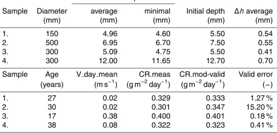
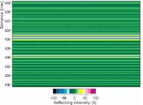
the water main was build (GOST 3262-75, 9567-75, 1050-88). In Fig. 2 an example of actual depth measurement of pipe wall by means of reflected ultrasonic sound is shown. For each example 7 depth measurements were taken using method shown in Fig. 2. The depth reading shown in Fig. 2 is 430.0–425.6=4.4 mm. The actual pipe wall depth measurement was taken between 2 or more reflection horizontals. For all

5

pipe examples the average and minimal values of pipe wall depths was calculated. By subtraction of the initial depth, taken from manufacturing standards, and measurement, the average and the maximal decrease in pipe wall depth were obtained. Since the corrosion formulas in the model were calculated from data of average loss of mass, the average decrease in pipe wall depth was used for model validation. Maximal decrease

10

of pipe wall depth was expressed as a linear function of average decrease. In further model simulations the maximal decrease was used since the time of the first breakage will occur from maximal corrosion rate.

Measurements were done using wet ultrasonic 5 MHz sensor which is used for com-posite materials. For depth readings raw ultrasonic reflective signal was used (without

15

applying any filter) since applying filter for material surface with corrosion, containing micro air pours, signal will be not detectable. Initially the calibration of measurement device by changing sound expanding velocity in metal for polished steel pipe segment, with known depth measured by micrometer was done. It was found that measurements taken by the device and manually by the micrometer were similar at 5700 m s−1speed

20

(7)

DWESD

5, 85–120, 2012

M. Bernats et al.

Title Page

Tables Figures

◭ ◮

Back Close

Full Screen / Esc

Discussion

P

a

per

|

Dis

cussion

P

a

per

|

Discussion

P

a

per

|

Discussio

n

P

a

per

|

2.4 Measurement converting methodology

Depth measurements were converted to actual corrosion rate (CR.meas) with following methodology:

Loss of mass₌(hinitial−hmeas)·2πr·1·ρ=[t]

Per square meter=1.(2πr·1)=[m2]

5

Per day=365×years=[day]

CR.meas=

((hinitial−hmeas)·2πr·1·ρ·(2πr1·1)×10 6

)

365×(years−1)

=(hinitial−hmeas)·ρ×10

6

365×(years−1) (g m

−2_day−1₎ ₍₁₎

whereh_initial is initial depth of pipe wall from standards (m), h_meas – actual depth of pipe wall measurements (m), r – inner radius of pipe (m), 1 – longitudinal length of

10

circumference for accuracy of dimensions (m),ρ– density of metal used in pipe man-ufacturing, years – number of years pipe being in service.

Multiplying equation by inverse circumference was based on fact that for each full square meter the lengths of both longitude and latitude should be 1, so on either side dimensions are square meters and circumference in denominator works as

normaliza-15

tion of lost quantity of mass per square meter, reducing its value if circumference gives more than one or increasing its quantity if circumference gives less than one square meter. Data about pipe exploitation ages were collected from the archive of maintains enterprise of water supply network. The corresponding metal densities were described in manufacturing standards, with small variations in their value and generally being

20

(8)

DWESD

5, 85–120, 2012

M. Bernats et al.

Title Page

Tables Figures

◭ ◮

Back Close

Full Screen / Esc

Discussion

P

a

per

|

Dis

cussion

P

a

per

|

Discussion

P

a

per

|

Discussio

n

P

a

per

|

2.5 Validation methodology

For validation of model corrosion rate (CR.mod) by measurements was done following methodology of Eqs. (2) and (3). It is mentioned that (CR.meas) of measurement is expressed from total lost mass, thus including first year corrosion constant (C).

CR.mod×365 (years−1)+C≈Measurement (total lost mass);

5

Since interest is about second stage corrosion rate (after first year constant),

CR.mod≈Measurement−C 365 (years−1)

After CR.model approximation on measurements,

CR.mod·X1∼₌ Measurement 365 (years−1)

[CR.mod.v1×365 (years−1)·X1+C∼₌Measurement (forv≤0.1 m s−1) (2)

10

[CR.mod.v2×365 (years−1)·X2₊C∼₌Measurement (forv >0.1 m s−1) (3) where CR.mod.v1 is the corrosion rate for flow region 1 (v≤0.1 m s−1), CR.mod.v2 – corrosion rate for flow region 2 (v >0.1 m s−1), X1 – approximation function for the corrosion rate of flow region 1,X2 – approximation function for corrosion rate of flow

15

(9)

DWESD

5, 85–120, 2012

M. Bernats et al.

Title Page Abstract Introduction Conclusions References Tables Figures ◭ ◮ ◭ ◮ Back Close

Full Screen / Esc

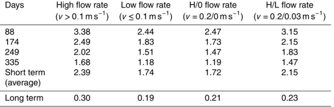
Printer-friendly Version Interactive Discussion Discussion P a per | Dis cussion P a per | Discussion P a per | Discussio n P a per | 3 Results

Exact model approximation on the corrosion process measurements is shown in Fig. 4. Two stages of corrosion process, in respect to time, were selected. In the first 360 days, the corrosion advances in considerably higher rate while the oxygen-limiting layer is formed. This step shows a semi-linear trend, with a gradual decrease of the slope.

5

Since this stage has fixed time value till which it applies, it can be expressed as constant in long term simulations. In the model this constant was called first year constant (C_high for “high flow rate” and Clow for “low flow rate”). After the first 360 days the stage

2 starts, where corrosion happens at a lower rate and with constant value (CRhigh for

“high flow rate” and CR_lowfor “low flow rate”). The numerical values of Fig. 4 are shown

10

in Table 2.

Based on approximated experimental data of rig tests, the corrosion rate expressions for stage 2 were established. The long term corrosion rate expressions were set as function only from mean hour flow velocity which changed the water temperature, all rest chemical parameters assuming constants.

15

Corrosion expressions established from corrosion rig tests are listed below, Eqs. (4) and (5), the dimensions are g m−2day−1(losed quantity, per square meter, per day).

CR.mod.v1=0.27×10

10

(Cl −

+2SO2−

4

alk ) 0.4

×e−(6000/(273+T)) (pH−5)·Ca0.2

(forv≤0.1 m s−1) (4)

CR.mod.v2=0.65

×1010(Cl −

+2SO2₄−

alk ) 0.2

×e−(6000/(273+T))

pH·Ca0.1 (forv >0.1 m s −1

) (5)

20

(10)

DWESD

5, 85–120, 2012

M. Bernats et al.

Title Page

Tables Figures

◭ ◮

Back Close

Full Screen / Esc

Discussion

P

a

per

|

Dis

cussion

P

a

per

|

Discussion

P

a

per

|

Discussio

n

P

a

per

|

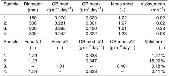
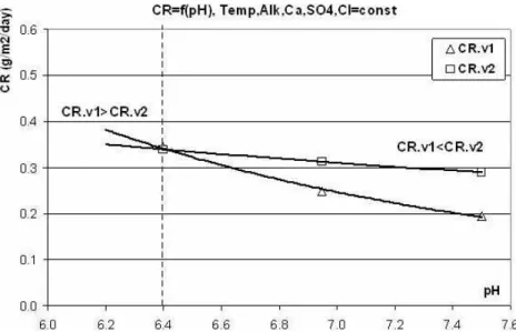
The difference function graphic is shown in Fig. 5 and the corresponding numerical values are shown in Table 3. For each flow region a di_fferent function was approx-imated. It is important to note that the relation between corrosion rates CR.mod.v1 (v≤0.1 m s−1) and CR.mod.v2 (v >0.1 m s−1) is not constant, i.e. for value pH≤6.45, CR.mod.v1>CR.mod.v2, but for pH>6.45, CR.mod.v1<CR.mod.v2. Generally pH

5

value of≤6.45 characterizes surface water, but pH value of>6.45 underground waters. The interrelation between CR.mod values as function of pH is shown in Fig. 6.

In Fig. 7 the error range of initial and validated corrosion model is shown. The corre-sponding numerical values and additional information about pipe samples are shown in Table 4. The maximal corrosion rate as function from average corrosion rate is shown

10

in Fig. 8. After model validation with average corrosion rates the maximum corrosion rate values were used for long term simulations.

There is a linear, positive relationship, between the corrosion rate (established from measurements) and flow velocities (determined from validated hydraulic model), e.g. CR (rate, g m−2day−1)=0.24 (velocity, m s−1)+0.31 (Fig. 9).

15

Corrosion expressions after validation are as follows:

[CR.mod.v1×365 (years−1)]·(1.7 ¯v+1.2)+C(forv≤0.1 m s−1

) (6)

[CR.mod.v2×365 (years−1)]·(0.82 ¯v−0.22

)+C(forv >0.1 m s−1

) (7)

where CR.mod.v1 and CR.mod.v2 is initial corrosion expressions, Eqs. (4) and (5)

20

(g m−2day−1), years – number of years pipe being in service, ¯ν– average flow velocity (m s−1), C – first year constants, forν≤0.1 m s−1 C=635 g m−2, for ν >0.1 m s−1 C= 785 g m−2.

4 Discussion

The values of validated model are the values of the initial model multiplied by diff

er-25

(11)

DWESD

5, 85–120, 2012

M. Bernats et al.

Title Page

Tables Figures

◭ ◮

Back Close

Full Screen / Esc

Discussion

P

a

per

|

Dis

cussion

P

a

per

|

Discussion

P

a

per

|

Discussio

n

P

a

per

|

and validated model error ranges are shown in Fig. 7. Initially model values versus measurement values fit relatively well, mostly because of the fact that the theoretical formulas were calculated from the same water supply network from which the pipe samples were taken, thus water chemical content remained constant. After the val-idation of the model the error was reduced to 15 %. The difference functions were

5

set so that the model after validation gives only positive error. Thereby the model is more reliable by giving a corrosion brakeage warning at maximum 15 % earlier, which involves noticeably less emergency costs than in a case of delayed brakeage warn-ing. The difference function X1 and X2 for the validated model were calculated as the difference ratio between measured value and the expected value obtained from the

10

model. Then difference ratio was plotted versus daily average flow velocity of hydraulic model and for each flow region (1. region v≤0.1 m s−1, 2. region v >0.1 m s−1) the difference function was calculated. The greatest difference between the model and the measurements is for the 1st region (v≤0.1 m s−1), therefore a linear difference func-tiony=1.7x+1.2 was found. In the case of flow velocityv=0 m s−1the initial model

15

value was increased by 20 %. A difference function for 2nd region (v >0.1 m s−1) was found y=0.82x−0.22

, which gradually joins to only point of 2nd region measurement. For 2nd region was chosen power function, because there is only one measurement point and it match good with model, so difference function should decrease more faster then linear function.

20

In Eqs. (4) and (5) is shown established corrosion rate expressions for both flow regions, Eq. (4) for v≤0.1 (m s−1), and Eq. (5) v >0.1 (m s−1). This system of two equations in respect to flow velocity is explained by observing different oxygen trans-ferring quantity between water flow and corrosion layer. This di_fferent oxygen trans-ferring quantity does not have constant relationship between both corrosion Eqs. (4)

25

(12)

DWESD

5, 85–120, 2012

M. Bernats et al.

Title Page

Tables Figures

◭ ◮

Back Close

Full Screen / Esc

Discussion

P

a

per

|

Dis

cussion

P

a

per

|

Discussion

P

a

per

|

Discussio

n

P

a

per

|

region 2 (v >0.1 m s−1) is from pH≤6.45. Usually the water with pH≤6.45 is sur-face source water, while water with pH>6.45 comes from groundwater source, so in general groundwater will correspond to relationship CR.mod.v1<CR.mod.v2, but the surface water will correspond to relationship CR.mod.v1>CR.mod.v2. The maximal corrosion rate was expressed as linear function from average corrosion rate, based on

5

measurement data of pipe samples (Fig. 8).

The correlation between the corrosion rate (g m−2day−1) and the flow velocity (m s−1) is of special interest, since it establishes a direction of the corrosion process as function from flow velocity (Fig. 9). However this correlation is obtained only from the pipe samples of the rigth bank of network, which in accordance of the hydraulic model data,

10

generally is supplied by water WTP-B. Therefore the correlation in Fig. 9 is valid only for groundwater source supplied networks (pH>6.45). Theoretically the correlation between the corrosion rate and the flow velocity for network part supplied by WTP-D (surface water source, pH≤6.45) should be inversely negative to the correlation of Fig. 9.

15

Further results of corrosion model simulations, shown in appendix, are discussed. The corrosion rates of network links in the first year (A1, g m−2yr−1) and all forthcoming years after the first year (A2, g m−2day−1) are shown in the Appendix A. The all follow-ing data calculations were based on these values. The total corroded mass (g m−2) after the first year (B1), after the tenth year (B2), and after the thirtieth year (B3) is

rep-20

resented in Appendix B. The corrosion depths of pipe walls (mm), assuming that steel density used in pipes isρsteel=7.5 t m

−3

, after first year (C1), after tenth year (C2), and after thirtieth year (C3) are shown in Appendix C.

The most graphic effect of corrosion in water supply network can be seen in Ap-pendix C where after first year there was a jump in pipe wall decrease from which

25

(13)

DWESD

5, 85–120, 2012

M. Bernats et al.

Title Page

Tables Figures

◭ ◮

Back Close

Full Screen / Esc

Discussion

P

a

per

|

Dis

cussion

P

a

per

|

Discussion

P

a

per

|

Discussio

n

P

a

per

|

equal to 7.5 t m−3, gives the corresponding average decrease of actual pipe depth by 0.013/0.016 mm per year (0.1 mm per 6.2/7.5 yr). As mentioned before in the validated model simulations maximal corrosion rate was used since the pipe will break in point of maximal corrosion and in time of maximal rate. According to Fig. 8 maximal corrosion rate is the average rate multiplied by 1.80.

5

From model simulations it was calculated that corrosion safe exploitation period, for standard steel pipes, with clear metal thickness of 5.50 mm, which corresponds to com-mercial diameter range from DN100–DN300 mm, is in range of 30–35 yr. For further corrosion reducing studies, attention should be directed to methods which reduce the value of relationship CR.max/CR.mean in water treatment process, since by reducing

10

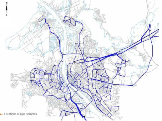
this ratio, the service time of water mains will proportionally increase. In the current study the validation of the corrosion model was done only for one bank of city water supply network (marked with arrows) which is supplied by groundwater source water from WTP-B. Consequently for the corrosion model validation in water supply network or its part supplied by surface water source additional validation should be done in the

15

future. It is important to note that the largest disadvantage of the field trials for con-sidered as a statically stable studies is the small number of validation measurements (n≪30). It is still believed that behavior of this corrosion model is correct, thereby with increase of sample number the accurateness of this model will increase.

5 Conclusions

20

From this study the following conclusions can be drown:

1. There is a significant positive correlation, for underground source water, between the corrosion rate on pipe wall inner surface and the flow velocity.

2. The surface source water causes approximately two times faster corrosion of a water supply network by means of the average corrosion rate, with the average

25

(14)

DWESD

5, 85–120, 2012

M. Bernats et al.

Title Page

Tables Figures

◭ ◮

Back Close

Full Screen / Esc

Discussion

P

a

per

|

Dis

cussion

P

a

per

|

Discussion

P

a

per

|

Discussio

n

P

a

per

|

corrosion rate 0.23 g m−2day−1, after the oxygen-limiting layer is formed in the first year.

3. Optimal time of exploitation, for commercial diameter range from diameter 100 to 300 mm, for cast iron and steel pipes is in range of 30–35 yr, if the initial metal layer thickness of the pipe wall is 5.50 mm.

5

4. The validated corrosion model, Eqs. (6) and (7) with error less than 15 % can be used for another water supply network, supplied by underground water source with similar water chemical properties to Riga city WTP-B. Otherwise the use of corrosion Eqs. (4) and (5) must be validated with approximation on field measure-ments.

10

Acknowledgements. This work has been undertaken as a part of the research project “Technol-ogy enabled universal access to safe water – TECHNEAU” (Nr. 018320) which is supported by the European Union within the 6th Framework Programme. There hereby follows a disclaimer stating that the authors are solely responsible for the work. It does not represent the opinion of the Community and the Community is not responsible for any use that might be made of

15

data appearing herein. Senior researcher (RTU) Janis Rubulis is gratefully acknowledged for valuable advices and guidance along the work. Kaspars Kalnins is gratefully acknowledged for significant measurement advices.

References

AWWA Research foundation: Internal corrosion of water distribution systems, Cooperative

re-20

search report, 2nd Edn., 1996.

AWWA Research foundation: Corrosion in a distribution system: steady water and its compo-sition, Water Res., 44, 1872–1883, 2010.

Juhna, T. and Osterhus, S. W.: Modelling of regrowth in water distribution network, TECHNEAU and SECUREAU Conference, 12 December 2009.

(15)

DWESD

5, 85–120, 2012

M. Bernats et al.

Title Page

Tables Figures

◭ ◮

Back Close

Full Screen / Esc

Discussion

P

a

per

|

Dis

cussion

P

a

per

|

Discussion

P

a

per

|

Discussio

n

P

a

per

|

Juhna, T., Gruskevica, K., Tihomirova, K., and Osterhus, S. W.: Influence of water velocity and NOM composition on corrosion of cast iron and copper, METEAU Conference, 29–31 October 2008.

Laycock, N., Laycock, P., Scarf, P., and Krouse, D.: Applications of statistical analysis tech-niques in corrosion experimentation, testing, inspection and monitoring, Shreir’s Corrosion,

5

chapter 2.36, 1547–1580, 2010.

McIntyre, P. J. and Mercer, A. D.: Corrosion testing and determination of corrosion rates, Shreir’s Corrosion, chapter 2.34, 1443–1526, 2010.

Naser, G. and Karney, B. W.: A 2-D transient multi component simulation model: application to pipe wall corrosion, Journal of Hydro-Environment Research, 1, 56–69, 2007.

10

Sarin, P., Snoeyink, V. L., Bebee, J., Kriven, W. M., and Clement, J. A.: Physico-chemical characteristics of corrosion scales in old iron pipes, Water Res., 35, 2961–2969, 2001. Vargas, I. T., Pasten, P. A., and Pizarro, G. E.: Empirical model for dissolved oxygen

de-pletion during corrosion of drinking water copper pipes, Corros. Sci., 52, 2250–2257, doi:10.1016/j.corsci.2010.03.009, 2010.

(16)

DWESD

5, 85–120, 2012

M. Bernats et al.

Title Page

Tables Figures

◭ ◮

Back Close

Full Screen / Esc

Discussion

P

a

per

|

Dis

cussion

P

a

per

|

Discussion

P

a

per

|

Discussio

n

P

a

per

|

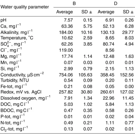
Table 1.Average values of water chemical parameters in WTP B and D.

Water quality parameter B D

Average SD± Average SD±

pH 7.57 0.15 6.91 0.26

Ca, mg l−1 63.36 5.75 52.13 6.28 Alkalinity, mg l−1 184.00 10.16 130.13 29.77 Temperature,◦C 10.62 2.59 8.65 8.03 SO2₄−, mg l−1 62.26 3.85 80.74 4.94 Cl−

, mg l−1

119.00 8.56

Mg, mg l−1 17.74 1.14 12.48 1.63 Mn, mg l−1 0.07 0.03 0.01 0.01 Si, mg l−1 2.99 0.79 2.15 1.13 Conductivity, µS cm−2

754.06 105.63 358.45 152.56 Turbidity, NTU 0.54 0.09 0.20 0.11 Fe-tot, mg l−1

0.21 0.08 0.05 0.00 Redox, mV vs. AgCl 257.82 30.80 260.61 127.02 Dissolved oxygen, mg l−1

7.91 1.34 22.96 11.45 DOC, mg C l−1 5.03 1.02 5.84 1.13 BDOC, mg C l−1 0.47 0.35 0.58 0.26 P-tot, mg l−1

0.01 0.01 0.02 0.04 N-tot, mg l−1

(17)

DWESD

5, 85–120, 2012

M. Bernats et al.

Title Page

Tables Figures

◭ ◮

Back Close

Full Screen / Esc

Discussion

P

a

per

|

Dis

cussion

P

a

per

|

Discussion

P

a

per

|

Discussio

n

P

a

per

|

Table 2. Numerical values of approximation of corrosion process (g m−2day−1) dynamics.

Days High flow rate Low flow rate H/0 flow rate H/L flow rate (v >0.1 m s−1

) (v≤0.1 m s−1) (v=0.2/0 m s−1

) (v=0.2/0.03 m s−1

)

88 3.38 2.44 2.47 3.15

174 2.49 1.83 1.73 2.15

249 2.02 1.51 1.47 1.83

335 1.68 1.18 1.19 1.47

Short term 2.39 1.74 1.72 2.15

(average)

(18)

DWESD

5, 85–120, 2012

M. Bernats et al.

Title Page

Tables Figures

◭ ◮

Back Close

Full Screen / Esc

Discussion

P

a

per

|

Dis

cussion

P

a

per

|

Discussion

P

a

per

|

Discussio

n

P

a

per

|

Table 3.Difference function values.

Sample Diameter CR.mod CR.meas Meas./mod. V day mean (mm) (g m−2day−1) (g m2day−1) (−) (m s−1)

1. 150 0.270 0.329 1.22 0.02

2. 500 0.281 0.301 1.07 0.02

3. 300 0.395 0.400 1.01 0.38

4. 300 0.242 0.322 1.33 0.08

Sample Func.X1 Func.X2 CR.mod·X1 CR.mod·X2 Valid error (−) (−) (g m−2day−1) (g m−2day−1) (−)

1. 1.23 – 0.333 – 1.27 %

2. 1.23 – 0.347 – 15.20 %

3. – 1.01 – 0.401 0.18 %

(19)

DWESD

5, 85–120, 2012

M. Bernats et al.

Title Page

Tables Figures

◭ ◮

Back Close

Full Screen / Esc

Discussion

P

a

per

|

Dis

cussion

P

a

per

|

Discussion

P

a

per

|

Discussio

n

P

a

per

|

Table 4.Pipe sample parameters and error range values.

Actual depth

Sample Diameter average minimal Initial depth ∆haverage

(mm) (mm) (mm) (mm) (mm)

1. 150 4.96 4.60 5.50 0.54

2. 500 6.95 6.70 7.50 0.55

3. 300 5.09 4.75 5.50 0.41

4. 300 12.00 11.65 12.70 0.70

Sample Age V day mean CR.meas CR.mod-valid Valid error (years) (m s−1) (g m−2day−1) (g m−2day−1) (−)

1. 27 0.02 0.329 0.333 1.27 %

2. 30 0.02 0.301 0.347 15.20 %

3. 17 0.38 0.400 0.401 0.18 %

(20)

DWESD

5, 85–120, 2012

M. Bernats et al.

Title Page

Tables Figures

◭ ◮

Back Close

Full Screen / Esc

Discussion

P

a

per

|

Dis

cussion

P

a

per

|

Discussion

P

a

per

|

Discussio

n

P

a

per

|

(21)

DWESD

5, 85–120, 2012

M. Bernats et al.

Title Page

Tables Figures

◭ ◮

Back Close

Full Screen / Esc

Discussion

P

a

per

|

Dis

cussion

P

a

per

|

Discussion

P

a

per

|

Discussio

n

P

a

per

|

(22)

DWESD

5, 85–120, 2012

M. Bernats et al.

Title Page

Tables Figures

◭ ◮

Back Close

Full Screen / Esc

Discussion

P

a

per

|

Dis

cussion

P

a

per

|

Discussion

P

a

per

|

Discussio

n

P

a

per

|

(23)

DWESD

5, 85–120, 2012

M. Bernats et al.

Title Page

Tables Figures

◭ ◮

Back Close

Full Screen / Esc

Discussion

P

a

per

|

Dis

cussion

P

a

per

|

Discussion

P

a

per

|

Discussio

n

P

a

per

|

(24)

DWESD

5, 85–120, 2012

M. Bernats et al.

Title Page

Tables Figures

◭ ◮

Back Close

Full Screen / Esc

Discussion

P

a

per

|

Dis

cussion

P

a

per

|

Discussion

P

a

per

|

Discussio

n

P

a

per

|

(25)

DWESD

5, 85–120, 2012

M. Bernats et al.

Title Page

Tables Figures

◭ ◮

Back Close

Full Screen / Esc

Discussion

P

a

per

|

Dis

cussion

P

a

per

|

Discussion

P

a

per

|

Discussio

n

P

a

per

|

(26)

DWESD

5, 85–120, 2012

M. Bernats et al.

Title Page

Tables Figures

◭ ◮

Back Close

Full Screen / Esc

Discussion

P

a

per

|

Dis

cussion

P

a

per

|

Discussion

P

a

per

|

Discussio

n

P

a

per

|

(27)

DWESD

5, 85–120, 2012

M. Bernats et al.

Title Page

Tables Figures

◭ ◮

Back Close

Full Screen / Esc

Discussion

P

a

per

|

Dis

cussion

P

a

per

|

Discussion

P

a

per

|

Discussio

n

P

a

per

|

(28)

DWESD

5, 85–120, 2012

M. Bernats et al.

Title Page

Tables Figures

◭ ◮

Back Close

Full Screen / Esc

Discussion

P

a

per

|

Dis

cussion

P

a

per

|

Discussion

P

a

per

|

Discussio

n

P

a

per

|

(29)

DWESD

5, 85–120, 2012

M. Bernats et al.

Title Page

Tables Figures

◭ ◮

Back Close

Full Screen / Esc

Discussion

P

a

per

|

Dis

cussion

P

a

per

|

Discussion

P

a

per

|

Discussio

n

P

a

per

|

Fig. A1.Corrosion rate constants (C) of 1st year (g m−2

(30)

DWESD

5, 85–120, 2012

M. Bernats et al.

Title Page

Tables Figures

◭ ◮

Back Close

Full Screen / Esc

Discussion

P

a

per

|

Dis

cussion

P

a

per

|

Discussion

P

a

per

|

Discussio

n

P

a

per

|

(31)

DWESD

5, 85–120, 2012

M. Bernats et al.

Title Page

Tables Figures

◭ ◮

Back Close

Full Screen / Esc

Discussion

P

a

per

|

Dis

cussion

P

a

per

|

Discussion

P

a

per

|

Discussio

n

P

a

per

|

(32)

DWESD

5, 85–120, 2012

M. Bernats et al.

Title Page

Tables Figures

◭ ◮

Back Close

Full Screen / Esc

Discussion

P

a

per

|

Dis

cussion

P

a

per

|

Discussion

P

a

per

|

Discussio

n

P

a

per

|

(33)

DWESD

5, 85–120, 2012

M. Bernats et al.

Title Page

Tables Figures

◭ ◮

Back Close

Full Screen / Esc

Discussion

P

a

per

|

Dis

cussion

P

a

per

|

Discussion

P

a

per

|

Discussio

n

P

a

per

|

(34)

DWESD

5, 85–120, 2012

M. Bernats et al.

Title Page

Tables Figures

◭ ◮

Back Close

Full Screen / Esc

Discussion

P

a

per

|

Dis

cussion

P

a

per

|

Discussion

P

a

per

|

Discussio

n

P

a

per

|

(35)

DWESD

5, 85–120, 2012

M. Bernats et al.

Title Page

Tables Figures

◭ ◮

Back Close

Full Screen / Esc

Discussion

P

a

per

|

Dis

cussion

P

a

per

|

Discussion

P

a

per

|

Discussio

n

P

a

per

|

(36)

DWESD

5, 85–120, 2012

M. Bernats et al.

Title Page

Tables Figures

◭ ◮

Back Close

Full Screen / Esc

Discussion

P

a

per

|

Dis

cussion

P

a

per

|

Discussion

P

a

per

|

Discussio

n

P

a

per

|